Transcriptional determinants of goal-directed learning and representational drift in the parahippocampal cortex

SUMMARY

Task learning involves learning associations between stimuli and outcomes and storing these relationships in memory. While this information can be reliably decoded from population activity, individual neurons encoding this representation can drift over time. The circuit or molecular mechanisms underlying this drift and its role in learning are unclear. We performed two-photon calcium imaging in the perirhinal cortex during task training. Using post hoc spatial transcriptomics, we measured immediate-early gene (IEG) expression and assigned monitored neurons to excitatory or inhibitory subtypes. We discovered an IEG-defined network spanning multiple subtypes that form stimulus-outcome associations. Targeted deletion of brain-derived neurotrophic factor in the perirhinal cortex disrupted IEG expression and impaired task learning. Representational drift slowed with prolonged training. Pre-existing representations were strengthened while stimulus-reward associations failed to form. Our findings reveal the cell types and molecules regulating long-term network stability that is permissive for task learning and memory allocation.

In brief

McLachlan and Lee et al. combined chronic population imaging in the perirhinal cortex during task training with post hoc spatial transcriptomics to identify neuronal cell types and measure immediate-early gene expression. They identified the cell types and molecules regulating long-term network stability that is permissive for task learning and memory allocation.

Graphical Abstract

INTRODUCTION

Goal-directed behavior involves learning how sensory stimuli and actions are related to possible outcomes. Neural circuits need to process such information, be flexible enough to adapt to new experiences, and be stable enough to retain learned relationships. How the mammalian cortex is organized to carry out these functions is an open question. Chronic recordings have enabled network stability and instability to be assessed in the context of learning and memory. Representational drift has been observed in different cortical areas wherein representations are reliably encoded at the population level, but the individual neurons encoding this information continuously change over days.^1–5 While theoretical models have speculated on the role of representational drift,^6–10 identifying specific circuits or molecular mechanisms that drive this phenomenon is critical for understanding how the stability and flexibility of neural representations relate to learning and memory.

Transcriptional profiling has produced molecular classifications that hierarchically subdivide neurons into major classes, subclasses, supertypes, and subtypes.^11,12 The unique, non-overlapping expression pattern of cell type genes (CTGs) defines each transcriptomic cell type. Recent experiments have demonstrated that a range of functional properties related to neural network state, sensory coding, and innate and goal-directed behaviors can be attributed to transcriptomic cell types.^13–16 Other classes of genes have been implicated in neural circuit function. Immediate-early genes (IEGs) have been investigated for their role in neuronal plasticity.¹⁷ Neural activity can drive IEG expression, which, in turn, can alter neural circuits to support learning and memory.¹⁸ Sensory coding has been shown to differ across neurons depending on IEG patterns.^13,19,20 IEGs have been used to tag neural populations encoding experiences and memories for later retrieval.^21–23 IEG induction patterns can both be restricted to specific cell types as well as span multiple cell types.²⁴ Despite this evidence, it is unclear to what degree neuronal functions related to learning and behavior can be ascribed to cell types, IEG expression, or both.

To disentangle how cell types and IEGs are involved in task learning and representational drift, we combined large-scale longitudinal population imaging with multiplexed spatial transcriptomics using a platform for Comprehensive Readout of Activity and Cell Type Markers (CRACK).¹³ Chronic imaging allows monitoring of how neural representations evolve over learning, while spatial transcriptomics allows simultaneous profiling of CTG and IEG expression in functionally characterized neurons. We applied this method to the perirhinal cortex (Prh), a parahippocampal region that is a zone of convergence between the sensory neocortex and the hippocampus.^25–27 Prh has roles in multiple sensory- and memory-related functions including unitizing features, assigning relational meaning, signaling novelty, and temporal ordering of stimulus items.^28–30 As a mesocortical area, Prh’s organization and cell type composition are distinct from the neocortex, archicortex (hippocampus), and paleocortex (amygdala). Whether learning and plasticity in Prh differ from these other cortical regions is unknown. We recently demonstrated that Prh is involved in forming stimulus-outcome associations during complex, goal-directed learning.³¹ IEGs involved in synaptic and structural plasticity have been implicated in associative learning in Prh.^32–36 CTGs have also been identified to delineate major neuronal subclasses and subtypes in Prh.^11,37 With these sets of genes, we sought to address how cell types, CTGs, and IEGs contribute to the formation and stability of learned task responses.

RESULTS

CRACK platform during task learning

To investigate how changes in neuronal responses during task learning relate to their transcriptional profile in Prh, mice were trained to perform a whisker-based delayed non-match-to-sample task that required them to classify sequentially presented whisker stimuli^13,38 (Figure 1A). A motorized rotor was used to deflect multiple whiskers in either an anterior (A) or posterior (P) direction during an initial “sample” and a later “test” period. Mice were trained to report whether the presented sample and test stimuli were non-matching or matching by licking or with-holding licks, respectively. Training was divided into multiple stages. The initial training stages consisted of one non-match stimulus condition (AP) and two match stimulus conditions (AA and PP). Training under these conditions was subdivided into 2 stages according to initial naive performance (T1) and learned performance (T2, dʹ >0.45 for two consecutive sessions). Completion of T2 required the animal to unitize the sample and test stimuli and pair it with reward. In the following stage (T3), the remaining held-out non-match condition (PA) was introduced, which required the animal to learn a new stimulus-reward contingency and generalize non-match and match across all possible combinations. Following successful learning of T3, delays between the sample and test stimuli were gradually extended up to 2 s (T4) to increase the temporal separation between sample and test stimuli. During the final stage (T5), the rotor was fully retracted during the delay period to require animals to retain a working memory of the sample stimulus. This also prevented the animal from relying on potential positional cues that existed during T4 when the rotor remained in whisker contact throughout the delay period.

Figure 1. CRACK platform during task learning in Prh.

(A) Schematic of a head-fixed two-photon imaging in Prh (left). Design of training stages for whisker-based delayed non-match-to-sample task (right).

(B) Example imaging area at denoted training stage and session number (top row). Mean activity sorted by stimulus condition (middle row) or choice (bottom row) for indicated neuron (yellow arrow).

(C) Registration of in vivo calcium imaged neurons to ex vivo tissue section across multiple rounds of HCR-FISH. Top: re-identified RCaMP1.07+ neurons from in vivo two-photon images (left), ex vivo confocal images of endogenous fluorescence (middle), and ex vivo confocal images of endogenous fluorescence of HCR-FISH transcripts (right). Yellow arrows indicate examples of re-identified neurons. Bottom: detected transcripts of inhibitory cell type genes (left), excitatory cell type genes (middle), and immediate-early genes (right).

(D) Gene expression patterns of L2/3 Prh excitatory and inhibitory cell subclasses and types determined from CTX-HPF scRNA-seq database (top) and of re-identified neurons from CRACK platform (bottom). Barcode scheme in CRACK platform precludes decoding of excitatory genes in classified inhibitory neurons and decoding inhibitory genes in classified excitatory neurons (dotted white line).

Scale bars: 50 μm (B, C). See also Figures S1–S3; Tables S1–S3.

To deploy the CRACK platform on L2/3 Prh, we performed chronic multi-depth two-photon calcium imaging over the course of training (Figure 1B). To non-invasively image Prh using an upright two-photon microscope, a 2 mm microprism was laterally implanted to provide optical access along the cortical surface using a long working-distance objective. Following the last T5 behavior session, the brain was extracted, and tissue encompassing the imaged volume was sectioned parallel to the imaging plane. The tissue was embedded in hydrogel and cleared for subsequent multiplexed hybridization chain reaction-fluorescence in situ hybridization (HCR-FISH) and confocal imaging (Figure 1C). To reidentify and register in vivo neurons across multiple rounds of HCR-FISH, we dedicated one imaging channel (561 nm) to repeated labeling and imaging of transcripts of the red genetically encoded calcium indicator, RCaMP1.07, which we used for functional imaging. Since cell type genes are characterized by non-overlapping expression patterns, we used a barcode labeling scheme for these genes optimized for non-overlapping detection across two imaging channels (488 and 785 nm) (Figure S1). Since IEGs could be potentially expressed in overlapping populations, we dedicated a fourth imaging channel (647 nm) to serially label individual IEGs. Overall, 23 genes were labeled over 9 rounds of staining.

To select genes delineating L2/3 cell types, we analyzed single-cell RNA sequencing (scRNA-seq) data acquired as part of a larger study of the molecular diversity of the isocortex¹¹ (Figure S1). Based on combinatorial expression patterns, excitatory L2/3 intratelencephalic (IT) pyramidal neurons in Prh were segregated into three transcriptomic supertypes: L2/3 IT CTX Trhr, L2/3 IT CTX Stard8, and L2/3 IT CTX Baz1a. For inhibitory neurons, we subdivided inhibitory subclasses (Lamp5, Vip, Sst, and Pvalb) into further subdivisions based on their abundance in Prh. Lamp5 neurons were subdivided into two subclasses according to the expression of neuron-derived neurotrophic factor (Ndnf) or CAC motif chemokine ligand 14 (Cxcl14). Vip, Sst, or Pvalb neurons were subdivided according to the expression of Cxcl14, prodynorphin (Pdyn), or tachykinin precursor 1 (Tac1), respectively. We selected 13 genes to identify the 3 excitatory supertypes and 8 inhibitory subclasses. In addition, we selected a panel of 9 IEGs whose cellular function has been characterized^17,39–42 and with known roles in Prh.^32,34–36 This includes insulin-like growth factor (Igf1), corticotropin-releasing hormone (Crh), activity-regulated cytoskeleton-associated protein (Arc), early growth response protein 2 (Egr2), neuronal PAS domain protein 4 (Npas4), brain-derived neurotrophic factor (Bdnf), neuronal pentraxin 2 (Nptx2), nuclear receptor subfamily 4 group A member 1 (Nr4a1), and c-Fos (Fos). Some IEGs were selectively enriched in Vip inhibitory subclasses and in L2/3 IT CTX Baz1a neurons, but all showed expression in individual neurons through all subtypes. Gene expression patterns and distributions across the analyzed population were consistent with that observed in the scRNA-seq data (Figures 1D and S2).

Goal-directed learning strengthens task-related subpopulations in Prh

To characterize task-related responses for each recorded cell across learning, we fit a generalized linear model (GLM) to each neuron’s estimated calcium event activity against a range of “task variables” (Figures 2A, S4, and S5). Task variables representing a related feature were grouped into “task factors” (Figure 2B). The ability for a neuron to encode a particular task factor was determined by calculating the difference in the Akaike information criterion (ΔAIC) between a full model and a partial model that excludes task variables representing that task factor. A positive ΔAIC value indicates reduced fit quality from the full to the partial model, revealing that the excluded task factor in the partial model is an important predictor of the modeled neuron’s activity. Thus, we interpret significant, positive ΔAIC values to indicate neuronal encoding of the excluded task factor. We analyzed 8 task factors. Three of the 8 task factors were defined by trial type. This included information related to the stimulus direction. Encoding of stimulus speed was also assessed as rotor deflections were delivered at different speeds (“fast” or “slow”) during trials. A task factor specific to Hit trials over the test and report period (Hit_TEST+REPORT) captured activity reflecting stimulus-reward associations. Additional task factors were used to describe tactile events during the trial period, including whisker-rotor touch onset and touch offset as well as phasic responses to the start and stop of the rotor rotation. A final task factor, coupling, was derived from the activity of all other simultaneously recorded neurons (see STAR Methods) to assess the level of coupling the neuron had with local network activity.⁴³

Figure 2. Single neuron encoding of task variables across learning.

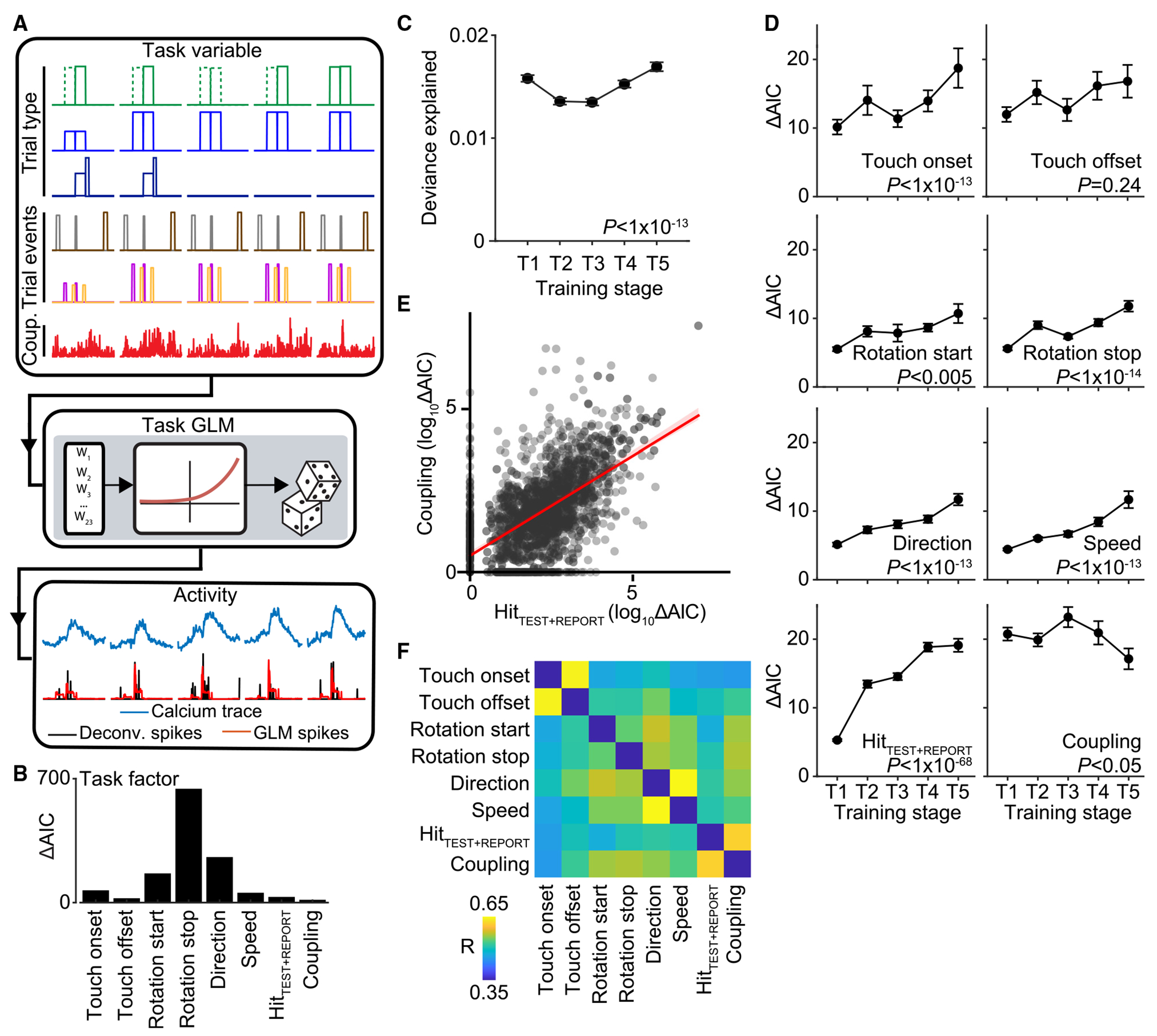
(A) Single neuron encoding of task-related activity within a single behavior session using a GLM.

(B) Encoding of task factors determined by comparing full and partial GLM fits (ΔAIC).

(C) Deviance explained for GLM across training stages. Deviance explained decreases during T2 and T3 but is unchanged between T1 and T5. Repeated measures ANOVA with post hoc multiple comparison test.

(D) Encoding strength of each task factor across training stages. All task factors, except for touch offset, strengthen with task training. Repeated measures ANOVA with post hoc multiple comparison test.

(E) Relationship between encoding of coupling and Hit_TEST+REPORT across the population during T5. Scatterplot shows individual neuron (black dots) and linear regression (red line) between the task factors.

(F) Relationship between all task factors across the population at T5. Correlation coefficient between each pair of task factors is shown, revealing three functional subpopulations encoding (1) touch onset and offset, (2) direction and speed, and (3) Hit_TEST+REPORT and coupling.

p values in (C) and (D) are from repeated measures ANOVA with post hoc multiple comparison test. Error bar: SEM. n = 953 neurons from 4 animals. See also Figures S4, S5, and S7.

We first assessed the GLM’s ability to explain neuronal responses across learning. The overall GLM fit (deviance explained) decreased slightly in T2 and T3 sessions overall, but no difference was observed when comparing the start (T1) and end (T5) of training (Figure 2C, p < 1 × 10⁻¹³, F_4,11515 = 17.78, repeated measures ANOVA with post hoc multiple comparison test). We next compared how individual task factor encodings change with learning (Figure 2D). Most sensory features except for touch offset increased their encoding strength with learning (touch onset: p < 0.02, F_4,11515 = 3.05, touch offset: p = 0.24, F_4,11515 = 1.39, rotation start: p < 0.005, F_4,11515 = 3.84, rotation stop: p < 1 × 10⁻¹⁴, F_4,11515 = 19.03, direction: p < 1 × 10⁻¹³, F_4,11515 = 17.14, speed: p < 1 × 10⁻¹³, F_4,11515 = 17.54, repeated measures ANOVA with post hoc multiple comparison test). Hit_TEST+REPORT exhibited the most dramatic increase in encoding strength across training stages (p <1 × 10⁻⁶⁸, F_4,11515 = 82.49, repeated measures ANOVA with post hoc multiple comparison test). Coupling was consistent over most training stages but decreased in T5 (p < 0.05, F_4,11515 = 2.63, repeated measures ANOVA with post hoc multiple comparison test).

To assess how individual neurons encoded multiple task factors across the population, we measured the degree to which the strength of a given task factor was correlated with the strength of another task factor (Figures 2E and 2F). We identified subpopulations of mixed-selective neurons. This included a subpopulation that encoded both touch onset and offset as well as a subpopulation that encoded both direction and speed. Neurons encoding Hit_TEST+REPORT were also likely to be functionally coupled to ongoing network activity. These task factor relationships were present throughout the course of training (Figure S7). Overall, these results indicate that task learning strengthens sensory and task-related information in Prh and that this information is encoded in distinct functional subpopulations.

Learned task responses are specific to cell types and transcriptional profiles

Having identified responses that emerge with task training and their functional organization, we next assessed the molecular composition of these subpopulations. Cell type classification segregates neurons into non-overlapping populations based on their aggregate gene expression pattern. However, we found that CTG expression can be heterogeneous when examining individual neurons (Figures S1A and S1C). A neuron classified as a given cell type might not necessarily express all the genes that define that cell type or can occasionally express genes that belong to another cell type. IEGs can be enriched in specific cell types but are also expressed across cell types. This raises the possibility that neuronal function could better be explained by expression patterns that are broader than those used for cell type classification. Given that spatial transcriptomics was performed at the end of behavior experiments, we focused our initial analysis on functional responses during expert T5 sessions prior to tissue extraction. For a given task factor, we fit a GLM to predict the distribution of encoding strengths across the neuronal population from each neuron’s cell type identity (cell type model) (Figures 3A and 3B). For comparison, we fit another GLM of the same task factor against each neuron’s transcriptional profile including CTGs and IEGs (gene model). GLMs were performed separately for each task factor.

Figure 3. Task encoding across cell types and genes in expert animals.

(A) Schematic of GLMs to predict encoding strength of one task factor of the neuronal population based on cell type classification (cell type model) or gene expression pattern (gene model).

(B) Example of predictive performance of GLM for touch offset using only IEGs on T5 sessions.

(C) GLM performance with the cell type model across task factors on T5 sessions. High deviance explained indicates that the task factor can be explained by cell type identity.

(D) GLM performance with the gene model across task factors on T5 sessions. High deviance explained indicates that the task factor can be explained by gene expression pattern.

(E) Comparison between cell type versus gene model across task factors on T5 sessions. Positive or negative ΔAIC indicates that task factor is better explained by gene expression or cell type identity, respectively.

(F) GLM performance with an IEG-only model across task factors on T5 sessions. High deviance explained indicates that the task factor can be explained by the IEG pattern.

(G) GLM performance with a CTG-only model across task factors on T5 sessions. High deviance explained indicates that the task factor can be explained by the CTG pattern.

(H) Comparison between CTG-only versus IEG-only model across task factors on T5 sessions. Positive or negative ΔAIC indicates that the task factor is better explained by IEGs or CTGs, respectively.

(I) Normalized covariate weights indicating the contribution of individual cell types to the cell type model across task factors on T5 sessions. Significant positive or negative weights relative to shuffled conditions indicate that the task factor is enriched or reduced, respectively, in each cell type.

(J) Contribution of individual genes to the gene model across task factors on T5 sessions. Significant positive or negative weights relative to shuffled conditions indicate that the task factor is enriched or reduced, respectively, in each gene.

(K) Relationship between gene expression for all task factors across the population at T5. Correlation coefficient between each pair of task factors is shown. n = 953 neurons from 4 animals.

See also Figure S6.

We first compared the model fit (deviance explained) between task factors. Model fit varied across task factors. For both the cell type and gene model, touch onset and offset showed higher deviance explained compared to other task factors suggesting this information could more readily be explained by cell type properties or gene expression patterns compared to other task information (Figures 3C and 3D). To determine whether cell type identities or transcriptional profiles were better at predicting a given task factor, we compared cell type versus gene models by calculating the ΔAIC between the model fits. Significant positive or negative ΔAIC values would indicate that task information could be better explained by transcriptional profile or cell type classification, respectively. A non-significant ΔAIC (ΔAIC < ∣14.07∣) would suggest that information could equally be explained by cell types and genes. For all task factors, we found that transcriptional profiles were better at predicting task factors than cell type identity (Figure 3E). Since the gene model contains both CTGs and IEGs, we sought to determine which sets of genes could better predict task information. We fit additional GLMs using either only CTGs or IEGs. For the CTG model, touch onset, speed, and Hit_TEST+REPORT showed higher deviance explained compared to other task factors (Figure 3F). For the IEG model, touch onset and offset showed higher deviance explained compared to other task factors (Figure 3G). When comparing the CTG and IEG model, we found that IEGs dominated the encoding of touch onset and offset (Figure 3H). For other task factors, the differences were less pronounced, suggesting that functional properties could be explained by a combination of CTGs and IEGs.

We next asked which cell types or transcriptional profiles encoded task information. This was done by comparing the normalized weights relative to shuffled conditions of each cell type or gene in their respective models. Significantly positive weights indicate that task information is enriched in specific cell types or related to increased expression of specific genes. Negative weights indicate that task information is absent in a specific cell type or related to decreased expression of specific genes. For the cell type model, we found that some task factors were enriched in one cell type (Figure 3I). Touch onset, touch offset, and rotation stop were significantly encoded in L2/3 IT CTX Baz1a neurons. Rotation start was encoded in Lamp5/Ndnf+ neurons. Coupling was encoded in L2/3 IT CTX Stard8 neurons. Speed was encoded in multiple types including L2/3 IT CTX Trhr and Lamp5/Ndnf+ neurons. Hit_TEST+REPORT was also encoded in multiple types including L2/3 IT CTX Baz1a, Pvalb, and Lamp5/Ndnf+ neurons.

For the gene model, we found more complex relationships in which combinations of CTGs and IEGs significantly contributed to task encoding (Figure 3J). For example, subpopulations encoding touch onset and offset consisted of neurons with increased expression of CTG (Sst) and IEGs (Crh and Arc) and decreased expression of CTGs (Gad2 and Ndnf) and IEG (Egr2). Neurons encoding Hit_TEST+REPORT showed increased expression of CTGs (Ndnf, Kit, Pvalb, Tac1, and 9533026P05Rik) and IEGs (Nr4a1 and Nptx2) and decreased expression of CTGs (Pdyn, Lypd1, and Adam2) and IEG (Bdnf). Cell type- and gene-specific differences in working memory responses were also observed (Figure S6). Comparison of expression profiles between task factors reinforces the presence of three subpopulations (Figure 3K). Touch onset and offset neurons shared similar expression patterns that were distinct from direction and speed neurons or Hit_TEST+REPORT and coupling neurons. These findings suggest that functional responses related to task learning in Prh are heterogeneous with respect to cell type classification and transcriptional profiles but can be clustered into three functionally and transcriptionally distinct subpopulations.

Learned task responses evolve differently across transcriptional profiles

Both gene expression and neural activity can change with learning. While the CRACK platform only provides a snapshot of gene expression at the end of training, this snapshot can still be related to the prior history of neural activity by chronic two-photon calcium imaging. Task responses may evolve differently across learning based on a neuron’s transcriptional profile. In the prior analysis, cell type and gene models were designed to identify the unique contributions of each component to task information. While CTGs and IEGs are often co-expressed, their trajectories across learning might not necessarily be coupled. Given the heterogeneous relationship between cell types, CTGs, IEGs, and encoded task factors in expert animals, we decided to analyze neural activity history for each gene independently. Neurons were divided into high- and low-expressing subpopulations. For each task factor, we then compared the encoding strength between the subpopulations at each training stage. Comparing the relative difference in ΔAIC between high- and low-expressing subpopulation controls for the overall strengthening of task factors during training, isolating changes that are specific to neurons based on gene expression (Figure 2D).

We found considerable reorganization in task-related activity across transcriptionally defined subpopulations (Figure 4A). Rotation start in Ndnf-expressing neurons was the only task response to be consistently present across all training stages. Among the three functional subnetworks, selective responses to touch onset and offset emerged in late training stages (T4–T5) among neurons expressing excitatory CTGs (Ccdc85b and 9530026P05Rik) and IEGs (Igf1, Crh, Arc, Npas4, Bdnf, and Fos) (Figure 4B). Direction and speed information were initially present in Ndnf-expressing neurons early during training (T1–T3), but later emerged in neurons expressing excitatory CTGs (Galnt14 and 9530026P05Rik). While Hit_TEST+REPORT and coupling are functionally correlated (Figures 2E and 2F), this information showed different time courses in changes across training. Hit_TEST+REPORT responses first emerged in Tac1- and Pvalb-expressing neurons (T3) and then Nptx2- and Nr4a1-expressing neurons (T4) (Figure 4C). Coupling was prominent in Nptx2- and Nr4a1-expressing neurons as early as T2 and was present in Bdnf- and Fos-expressing neurons in T5 but absent among Tac1- and Pvalb-expressing neurons. Overall, these findings indicate that learning-related changes in task information are heterogeneous across individual neurons but can be attributed to subpopulations based on their transcriptional profile.

Figure 4. Relationship between functional plasticity and terminal gene expression.

(A) Relative changes in encoding strength across training stages for neurons based on terminal gene expression across task factors. Significantly different encoding strengths are indicated. Student’s t test with Bonferroni-Holm correction.

(B) Examples of average activity traces across all trials from neurons with high (red) or low (black) expression of a given gene across training stages. Touch onset is denoted (dotted line). Sample period is shown in yellow. *indicates significantly different encoding strengths from (A). Touch onset responses are shown to emerge in neurons expressing Crh or Bdnf.

(C) Examples of average activity traces across Hit trials from neurons with high (red) or low (black) expression of a given gene across training stages. Sample period is shown in brown. * indicates significantly different encoding strengths from (A). Hit_TEST+REPORT responses are shown to emerge in neurons expressing Nptx2 or Nr4a1. Shaded region: SEM. n = 953 neurons from 4 animals.

Bdnf knockout in Prh impairs learning and alters network activity

The formation of stimulus-reward associations is a prominent aspect of task learning in Prh.^44–46 The emergence of Hit_TEST+REPORT and coupling responses among neurons expressing Bdnf, Nptx2, and Nr4a1 suggests that these IEGs are involved in stimulus-reward associations. Bdnf, Nptx2, and Nr4a1 have been shown to be part of a gene network involved in long-term synaptic and structural plasticity.^39–42,47 One possibility is that stimulus-reward activity patterns drive the expression of these genes. Another possibility is that these genes are necessary for the formation of stimulus-reward associations. We therefore asked whether disrupting this gene network in Prh could impair associative learning at both the behavioral and neuronal level.

We focused our genetic perturbation on Bdnf since it is an upstream regulator of Nptx2 and Nr4a1 expression. Using Bdnf^2lox mice,⁴⁸ viral vector expressing Cre recombinase was injected bilaterally in Prh to achieve conditional knockout (cKO) of Bdnf (Figure 5A). Viral vector expressing RCaMP1.07 was co-injected to image population activity in genetically perturbed neurons. We then performed microprism implantation and imaging during task training to compare functional differences between wild-type (WT) animals. At the end of the behavior experiments, HCR-FISH was performed on a subset of animals to confirm Bdnf knockout and to assess whether Nptx2 and Nr4a1 expression was altered across different cell types. To do this, we compared expression patterns in regions expressing RCaMP1.07 against neighboring regions. We verified that Bdnf expression was reduced in all cell types (Figure 5B). In addition, we observed decreased expression in many other IEGs including Nptx2 and Nr4a1 across multiple cell types. Increased expression of some IEGs was observed only in L2/3 IT CTX Trhr neurons. We then examined the effects of perturbed IEG expression on behavior. Animals were trained for up to 26 sessions. We observed impaired task learning compared to WT animals (p < 0.05, F_1,25 = 6.42, repeated measures ANOVA) (Figure 5C). While most WT animals (74%) were able to advance to T4 after 26 sessions, only 14% of Bdnf cKO animals could do so (Figure 5D). This demonstrates that task learning depends on IEG expression that is regulated by Bdnf in Prh.

Figure 5. cKO of Bdnf alters task learning, IEG expression, and neural coding.

(A) Targeted cKO of Bdnf induced by bilateral injection of Cre- and RCaMP1.07-expressing virus into Prh in Bdnf^2lox mice. Low-magnification ex vivo images of RCaMP1.07 and Bdnf expression at or next to the injection site (right, scale bar: 20 μm). High-magnification images of selected regions along with detected IEGs (lower left, scale bar: 10 μm).

(B) Relative difference in IEG expression between infected and non-infected neurons across cell type. Reduced IEG expression is observed across multiple cell types. Significant differences in expression are denoted. Student’s t test with Bonferroni-Holm correction.

(C) Task performance for WT and Bdnf cKO animals across 26 sessions. Performance for individuals and mean performance for the two groups are shown. Bdnf cKO animals show decreased performance compared to WT animals.

(D) Percentage of animals completing each learning stage after 26 sessions for WT and Bdnf cKO animals. Fewer Bdnf cKO animals reached T3 and T4 stages compared to WT animals.

(E) Comparison of deviance explained between WT and Bdnf cKO animals for task encoding GLM across T1 and T2 stages.

(F) Comparison of encoding strengths between WT and Bdnf cKO animals for each task factor across T1 and T2 stages.

(G) Example of population activity in WT and Bdnf cKO animals illustrating differences in population coupling. Increased synchronous activity observed in Bdnf cKO animals. Dotted red line demarcates different trials.

*p < 0.005, **p < 1 × 10⁻⁹, ***p < 1 × 10⁻²⁰ Student’s t test with Bonferroni-Holm correction (E and F). Shaded region: SEM (C). Error bars: SEM (E and F). n = 36,350 neurons from 4 Bdnf cKO animals (B), 11 WT animals, and 7 Bdnf cKO animals (C and D); 2,304 neurons from 7WT animals; and 1,285 neurons from 4 Bdnf cKO animals (E and F). Scale bar: 20 μm (A). See also Figure S3.

To understand how Prh activity differs between WT and Bdnf cKO mice, we first used GLMs to compare single-cell responses between animals. Since the majority of Bdnf cKO mice could not advance past T2, activity was only compared during T1 and T2 stages. Interestingly, we found that activity in Bdnf cKO mice could be better explained by the GLM compared to WT animals across both training stages (Figure 5E). The model fit also improved in Bdnf cKO mice from T1 to T2. This was reflected in a general increase in the encoding of all task factors including Hit_TEST+REPORT (Figure 5F). In particular, we found a dramatic increase in the encoding of coupling from T1 to T2, suggesting that population activity was more highly correlated in Bdnf cKO animals (Figure 5G). Overall, this indicates that cKO of Bdnf in Prh alters network activity and strengthens task information in single neurons during learning in an experience-dependent manner.

Bdnf knockout disrupts associative learning and reduces representational drift

The relationship between Hit_TEST+REPORT and coupling in WT animals suggests that stimulus-reward associations are encoded at a population level. The training-related increase in coupling in Bdnf cKO animals further suggests that Bdnf deletion alters this representation. To measure population-level representations of stimulus-reward associations, we trained a linear population decoder on activity during the report period using Hit vs. non-Hit trials. We cross-temporally (CT) tested the decoder’s performance on activity across other time points along the trial (Figure 6A). We assessed CT performance in WT animals, training a decoder on each behavior session. In early training sessions, the decoder could only discriminate reward information during the report period when reward was delivered (Figure 6B). However, as training progressed, we observed a gradual retrograde expansion of increased decoder performance earlier in the trial. This stretched into the test stimulus period when sufficient sensory information is available to predict reward. Analysis of the onset of decodable reward outcome across training stages showed that this expansion emerged as animals demonstrated learned performance (T2) and continued to expand through subsequent training stages (Figure 6C, p < 0.002, F_4,282 = 4.44, one-way ANOVA with post hoc multiple comparison test). Thus, this retrograde expansion suggests the formation of a stimulus-reward association. No such expansion was observed in Bdnf cKO animals (Figure 6C). The onset of decodable reward outcome was restricted to the report period and was delayed relative to WT animals at both T1 and T2 stages (p < 1 × 10⁻³: T1, p < 0.05: T2, Student’s t test with Bonferroni-Holm correction), suggesting that disrupting Bdnf expression impairs associative stimulus-reward learning in Prh.

Figure 6. Bdnf mediates associative learning and representational drift in Prh.

(A) Schematic of population linear decoders trained on Hit vs. non-Hit trials during the report period and tested on cross-temporal (CT) activity at different time points from the same session or cross-session (CS) activity on different sessions.

(B) Example of CT performance from a WT (left) and Bdnf cKO (right) animal across each task session. First decodable time point above chance is shown (white dot).

(C) CT onset time across training stages for WT and Bdnf cKO animals. Reward can be decoded earlier in the trial in WT animals but not in Bdnf cKO animals. **p < 0.001: T1, *p < 0.05: T2, Student’s t test.

(D) Example of CS performance to reward outcome from a WT (left) and Bdnf cKO (right) animal compared across each task session.

(E) CS decoder performance to reward outcome on the same (dotted) and following N+1 (solid) session for WT and Bdnf cKO animals across training stages. During T2, CS performance increases in Bdnf cKO animals. **p < 0.001: WT T2 vs. Bdnf cKO T2, ***p < 1 × 10⁻⁴: Bdnf cKO T1 vs. Bdnf cKO T2, Student’s t test.

(F) CS decoder performance to reward outcome trained on T2 sessions tested on subsequent N+i sessions for WT and Bdnf cKO animals. CS performance is stronger in Bdnf cKO animals across multiple session intervals. ***p < 1 × 10⁻¹¹, F_1,338 = 53.32, two-way ANOVA.

(G) CS decoder performance to touch onset on the same (dotted) and following N+1 (solid) session for WT and Bdnf cKO animals across training stages. CS performance is greater for Bdnf cKO animals on T1 and T2 sessions. **p < 0.001: WT T1 vs. Bdnf cKO T1, ***p < 1 × 10⁻⁴: WT T2 vs. Bdnf cKO T2, Student’s t test.

(H) CS decoder performance to touch onset trained on T2 sessions tested on subsequent N+i sessions for WT and Bdnf cKO animals. CS performance is stronger in Bdnf cKO animals across multiple session intervals. ***p < 1 × 10⁻¹⁹, F_1,335 = 96.92, two-way ANOVA.

Error bars: SEM. Red and black lines indicate 95^th percentile of shuffled performance for (E)–(H). n = 70 T1 sessions, 75 T2 sessions, 30 T3 sessions, 79 T4 sessions, and 48 T5 sessions from 7 WT animals and 60 T1 sessions and 24 T2 sessions from 4 Bdnf cKO animals. See also Figure S7.

Disrupted associative learning at the population level could occur either due to network hypo-stability, preventing memory consolidation, or hyper-stability, preventing adaptation to new experiences. To assess network stability related to representational drift, a linear population decoder for reward outcome was trained on activity during the report period using Hit vs. non-Hit trials from one session and its performance was tested on activity from other sessions (Session_ReportN+i) across learning (Figure 6A). The performance of these decoders when tested on trials from the same session consistently performed with >96% accuracy in both Bdnf cKO and WT animals, demonstrating that reward outcome is reliably represented in Prh (Figures 6D and 6E). We then assessed network stability by measuring cross-session (CS) performance in the next session (N+1). In WT animals, CS performance ranged from 73.0% to 78.8% for T1–T5 sessions, suggesting a drift in the neurons encoding reward outcome. No differences in session-to-session performance were found between training stages (Figure 6E, p = 0.19, F_4,260 = 1.54, one-way ANOVA), suggesting that the rate of drift was steady throughout learning. CS performance between Bdnf cKO (76.8% ± 1.6%, mean ± SEM) and WT (73.0 ± 1.7%) animals was initially similar during T1 sessions (p = 0.23, Student’s t test). However, once Bdnf cKO animals reached T2, CS performance increased significantly to 89.9% ± 0.9% (p < 1 × 10⁻⁴: Bdnf cKO T1 vs. Bdnf cKO T2, Student’s t test), which was also higher than WT (76.5% ± 1.8%) animals at the same training stage (p < 0.001: WT T2 vs. Bdnf cKO T2). We assessed CS performance across increasing intervals during T2 with respect to the second (N+2), third (N+3), fourth (N+4), and fifth (N+5) session interval. Representations of reward outcome were consistently more stable in Bdnf cKO animals compared to WT animals (Figure 6F, p < 1 × 10⁻¹¹, F_1,338 = 53.32, two-way ANOVA). Analysis of stability of touch onset showed that CS performance was higher for Bdnf cKO animals for both T1 (Bdnf cKO: 70.9% ± 1.8%, WT: 62.1% ± 1.4%, p < 1 × 10⁻³, Student’s t test) and T2 (Bdnf cKO: 78.7% ± 3.4%, WT: 65.2% ± 1.2%, p < 1 × 10⁻⁴, Student’s t test) stages (Figure 6G). CS performance was also consistently higher at longer session intervals (Figure 6H, p < 1 × 10⁻¹⁹, F_1,335 = 96.92, two-way ANOVA). Taken together, these findings demonstrate that representational drift is essential for associative learning. Altered IEG expression from deletion of Bdnf produces an inflexible network in which prior representations are stabilized and strengthened while newer stimulus-reward associations are incapable of forming.

DISCUSSION

Representational drift has been prominently observed across multiple cortical areas including sensory cortices, motor cortex, association cortex, and the hippocampus.^1–5 Depending on the cortical area, experience can influence the degree and rate of drift. The role of this drift in the context of learning and memory has been an open question. It has been proposed that maintaining a balance between plasticity and stability in the network allows memories to be reorganized for optimal storage.^49,50 In this manner, drift could allow for the integration of new associations and experiences without interfering with prior learned associations. Prh is an area involved in processing sensory information, distinguishing novel versus familiar stimuli, and associating stimuli with outcomes.^28–30 We have also shown that stimulus-reward associations in Prh can be compressed into abstract representations.⁴⁴ Leveraging recently acquired transcriptomic cell atlas data,^11,37 we were able to dissect the Prh circuits and genes involved in task acquisition. We demonstrate that representational drift is necessary for associative learning and that specific subsets of IEGs govern this process.

We find that goal-directed learning strengthens and organizes task information into distinct functional subpopulations in Prh. While we observe functional specificity among putative molecular cell types, a more comprehensive incorporation of gene expression demonstrates that learned task information in Prh spans multiple transcriptional axes consisting of genes defining cell types and those associated with neural plasticity. While some sensory information such as direction and speed responses are more strongly associated with specific cell types than by IEG expression, touch onset and offset are associated with the broad expression of multiple IEGs. Stimulus-reward associations are encoded across multiple cell types including Lamp5/Ndnf+, Pvalb, and L2/3 IT CTX Baz1a neurons. The activity patterns of these neurons are strongly coupled, operating as a subnetwork for representing such task information at a population level. Lamp5/Ndnf+ and Pvalb neurons have been implicated in a disinhibitory circuit that can regulate the excitability of cortical columns in a state-dependent manner.⁵¹ Activation of Lamp5/Ndnf+ neurons has been implicated in associative learning.⁵² We speculate that the ability for this circuit to modulate network activity may be permissive for stimulus and reward information to be combined into relevant associations.

Within this subpopulation, we find that IEGs form a gene network whose expression across the circuit is necessary for stimulus-reward learning. Our ability to multiplex gene measurements allows us to identify co-expressed genes including Nr4a1, Nptx2, and Bdnf whose endpoint expression is correlated with neurons that form stimulus-reward associations. Nr4a1 has been shown to regulate the distribution and density of dendritic spines on excitatory pyramidal neurons.⁴⁰ Nptx2 has been shown to strengthen excitatory synapses on Pvalb neurons.³⁹ Both genes are regulated by Bdnf,^41,42 which is also involved in both excitatory and inhibitory synaptic plasticity.⁴⁷

While we were not able to track gene expression changes during learning, we were able to provide evidence that these genes are causally involved in learning through conditional Bdnf knockout. Bdnf deletion in Prh altered the expression of Nr4a1, Nptx2, and other IEGs, confirming that IEGs including Bdnf are members of an inter-regulated gene network. Disruption of this gene network impaired task learning and altered task-related neural activity in an experience-dependent manner. While there were modest differences in task coding between Bdnf cKO and WT animals during T1 sessions, task information and network synchrony dramatically increased in Bdnf cKO as mice reached T2 sessions. This demonstrates that changes in activity in Bdnf cKO mice are related to task learning and not a general network deficit.

The rate of representational drift has been shown to depend on experience. In the post-parietal cortex, drift has been shown to increase with new learning stimulus associations under task conditions.¹ However, in the olfactory cortex, conditioned stimulus learning did not change drift rates while passive exposure to olfactory stimulus decreased drift.² In visual cortex, drift rates can also depend on stimuli.³ Thus, the relationship between representational drift and learning is not straightforward. Our study examines representational drift in mutant animals. We find that representational drift in Bdnf cKO animals is altered in a stimulus- and experience-dependent manner. While representations of whisker touch showed reduced drift rates throughout all of training, representations of reward outcome only decreased when animals advanced to T2. The formation of stimulus-reward associations was also disrupted during this period. The fact that deficits in both representational drift and associative learning were observed in Bdnf cKO animals strongly suggests that both these processes depend on Bdnf and related IEGs.

This suggests that plasticity is altered in such a way that pre-existing representations such as touch and reward outcome are reinforced while new representations such as stimulus-reward association are prevented from being incorporated into memory. We speculate that this disruption in memory allocation could be a result of a hyper-rigid network due to loss of Bdnf and related genes, which normally could allow for learning of new associations by reorganizing prior associations in a circuit-specific manner. The cellular mechanisms driving these changes remain to be determined but could involve changes in inhibition or synaptic plasticity, where Bdnf has known roles.^47,53,54 This can be investigated in future studies. Overall, this work demonstrates that the ability for circuits to adapt during learning and to store information in memory requires a continuous process that is reflected in the flexibility and stability of neural representations.^49,50

Limitations of the study

One limitation to the Bdnf knockout experiments is that the results were compared to WT animals but not control littermates, so potential background strain-specific differences between experimental groups cannot be completely ruled out. However, internal controls comparing adeno-associated virus-injected and non-injected regions show that Bdnf deletion in Prh altered the expression of Nr4a1, Nptx2, and other IEGs.

Another limitation to this study is that we were unable to track the temporal dynamics of the IEG expression. Therefore, it is not known whether the expression of IEGs identified at the end of the behavior experiments was present throughout training or only transiently expressed. Future studies, in which fluorescent reporters driven by specific IEG promoters are used, can allow us to investigate expression dynamics one gene at a time.^19,55

Conclusion

In summary, the function of neurons in a circuit can be informed by their transcriptional profile both from genes that define their cell type identity and from genes that enable their plasticity. By comprehensively linking CTGs and IEGs to network activity patterns, we can build an understanding for how circuits are organized to learn behaviorally relevant information and how molecular programs enable this learning to occur.

RESOURCE AVAILABILITY

Lead contact

Further information and requests for resources and reagents should be directed to and will be fulfilled by the lead contact, Jerry Chen (jerry@chen-lab.org).

Materials availability

HCR-FISH probes generated for this study are available through Molecular Instruments, Inc.

Data and code availability

• The processed data (spike times, probe locations, behavior, orofacial movements) have been deposited at GIN Node and are publicly available at https://doi.org/10.12751/g-node.8yt6sr.

• All original code used to analyze the data has been deposited at GIN Node and is publicly available at https://doi.org/10.12751/g-node.8yt6sr.

• Any additional information required to reanalyze the data reported in this paper is available from the lead contact upon request.

STAR★METHODS

EXPERIMENTAL MODEL AND STUDY PARTICIPANT DETAILS

Experiments in this study were approved by the Institutional Animal Care and Use Committee at Boston University and conform to NIH guidelines. Wild-type animal experiments were performed using C57BL/6J mice (The Jackson Laboratory). Bdnf conditional knockout experiments were performed using Bdnf^2flox/J mice (The Jackson Laboratory, #004339).⁴⁸ All animals (male and female) were 6–8 weeks of age at time of surgery. Mice used for behavior were housed individually in reverse 12-h light cycle conditions. All handling and behavior occurred under simulated night time conditions.

METHOD DETAILS

Preparation for animal imaging

Prh was targeted stereotaxically (2.7 mm posterior to bregma, 4.2 mm lateral, and 3.8mm ventral). For wild type animal experiments, a unilateral injection was targeted via the temporal bone at 250 μm and 500 μm below the pial surface with AAV.PHP.eB-EF1α-R-CaMP1.07 (600nL, 6.0x10¹² vg/mL). For Bdnf cKO animal experiments, animals received bilateral injections of 600nL of AAV.PH-P.eB-EF1α-RCaMP1.07 (6.0x10¹² vg/mL) and AAV1-hSyn-Cre-WPRE-hGH (7.0x10¹² vg/mL). For optical access, an assembly consisting of a 2mm aluminum-coated microprism (MPCH-2.0, Tower Optical) adhered to coverglass along the hypotenuse and the side facing Prh was implanted over the pial surface. A metal headpost was implanted on the parietal bone of the skull to allow for head fixation.

Behavior task training

Two weeks after microprism implantation and injections, animals were handled and acclimated to head fixation. Training to a head-fixed whisker-based context-dependent sensory task was performed similar to as described.³⁸ Whiskers were trimmed to a single row for videography. Animals were trained for two sessions per day. A go/no-go task design was used in which animals licked for water reward for non-match stimulus conditions and withheld licking for match stimulus conditions. The same task settings defining each of the 5 training stages (Table S1) were consistently applied across all animals to ensure that behavioral performance could be compared across experimental groups.

T1-T2 training stages required the animals to distinguish a single non-match condition (AP) from two match conditions (AA, PP). During T1, the proportion of non-match versus match trials were gradually changed from 0.9/0.1 to 0.5/0.5 (non-match/match) over the course of the first 5 T1 sessions. The purpose of this was to acclimate the animals to licking for reward and to avoid miss trials by providing a high proportion of rewarded (non-match) stimulus trials and gradually exposing animals to the non-rewarded (match) stimulus trials. Transition from T1 to T2 required that animals perform at d’>0.45 for two consecutive sessions. This reflects a change from naive to learning performance. No task settings were changed during this period. The second non-match condition (PA) was introduced in T3. Transition from T2 to T3 where the PA stimulus is introduced required that animals perform at d’>1.68 for two consecutive sessions.

Transition from T3 to T4 where the delay period is introduced required that animals perform at d’>0.168 for two consecutive sessions. During T4, the delay between the sample and test stimulus was gradually increased through a progression of sub-stages. An initial delay was used at the beginning of the session. Behavioral performance was measured every 15 trials. The delay was increased by a defined increment if performance exceeded >85% correct (d’ > 2.07) over the past 15 trials up to a maximum of 2 s. If the overall performance for the session was d’>1.68, the animal advanced to the next T4 sub-stage in which the starting delay and increment was greater than that used in previous session. The rotor was withdrawn once animals could begin sessions with delays of 2 s. During T5, delays were randomly varied between 2, 3, and 4 s to examine sequential activity across varying delay periods.

For T4, the delay between sample and test stimuli was gradually increased from 100ms to 2s with the rotor remaining within whisker reach throughout the delay period. For T5, the rotor was retracted 1.5cm during the delay period across delays of 2s, 3s, and 4s which were randomly presented with probabilities of 50%, 25%, and 25% respectively. Fast (1.75 cm/s) and slow (0.87 cm/s) rotations of stimulus direction were used. For T1-T4, slow directions represented 5% of all trials. For T5, the fraction of slow trials was increased to 25% of all trials.

Adjustments to task settings to reinforce correct behavioral choice were carried out semi-automatically. Punishment in the form of a combination of time outs (2-10s) and air puffs (100ms) ranging from 1 to 5 trains to the face was manually adjusted to discourage false alarm licking on match trials. During T1, the probability of non-match stimulus conditions was manually reduced to 35–40% of all trials reduce false alarm trials or increased up to 60% to reduce miss trials. Occasionally, behavioral lapses were also observed in which animals demonstrated correct choice strategies across extended trial periods but then reverted to incorrect choice strategies. Incorrect choice strategies were categorized as report bias, sample bias, and test bias. A set of task parameters were included in the training protocol to identify and correct for these biases without changing the stimulus-reward contingency (Table S2).

A report bias was defined as persistent licking of the lick port regardless of stimulus condition quantified as a high fraction of total hit and false alarm trials. Depending on the severity of the report bias, two corrective strategies were adopted. The first strategy is the use of punishment to discourage licking of the incorrect stimulus condition. Punishment consisted of a combination of time out and air puffs to the face. Initially introduced punishment was mild and gradually became more severe with longer time outs and multiple air puffs considered as more severe punishment. Tolerance for punishment can vary for individual animals (data not shown). For both task conditions, animals disengaged from the task if punishment was too aversive, resulting in miss trials. Punishment levels are reduced if misses increase. In addition to adjusting punishment levels, the probability of stimulus conditions was also adjusted to increase the frequency of the incorrect stimulus condition in order for animals to “practice” the correct response. Typically, non-match and match stimulus conditions were presented at 50% probability. This was increased up to 80% for the incorrect stimulus condition depending on the severity of the report bias.

A sample stimulus bias represented incorrect choice strategies in which the animal responded based on whether the sample stimulus was A or P. In contrast, a test stimulus bias represented incorrect choice strategies in which the animal responded based on whether the test stimulus was A or P. These biases were operationally defined as differences in performance between the two stimulus conditions belonging to the same category (AP vs. PA for non-match, AA vs. PP for match). Typically for each stimulus category, one of the two possible stimulus conditions is presented with 50% probability with respect to the other. To correct for sample or test bias, the probability of stimulus conditions belonging to the same category was adjusted to increase the frequency of the incorrect stimulus condition for animals to “practice” the correct response.

Animals only received water by performing the task. Their weight was monitored daily to ensure body weight did not drop below 80% of initial weight. Wild-type animals were trained continuously and terminated once animals had performed at least 4–6 T5 sessions. Bdnf cKO animals were trained for up to 26 sessions.

Two-photon imaging

A custom-built resonant-scanning multi-area two-photon microscope with a 10x/0.5NA, 7.77mm WD air objective (TL10X-2P, Thorlabs) using custom-written Scope software was used to perform 2-photon calcium imaging during head-fixed behavior.⁶³ A 31.25 MHz 1040 nm fiber laser (Spark Lasers) was used for RCaMP1.07 imaging. Imaging at 32.6 Hz frame rate was performed simultaneously of two imaging planes in L2/3 separated 50 μm in depth. Average power of each beam at the sample was 50-90mW. Following the conclusion of all experiments, animals were anesthetized and a high-resolution 3D image volume was taken through the imaged area for later registration with ex vivo tissue.

Ex vivo tissue preparation

For wild-type animals, tissue was extracted immediately following the end of the sixth T5 training session. For Bdnf cKO animals, tissue was extracted immediately following the end of the 26^th training session. The 2 mm aluminum-coated microprism was carefully removed. Several small punctures were made in tissue surrounding the in vivo imaged area using a glass pipette dipped in lipophilic dye (SP-DiIC₁₈(3) (1,1′-Dioctadecyl-6,6′-Di(4-Sulfophenyl)-3,3,3′,3′-Tetramethylindocarbocyanine; Fisher Scientific, cat no. D7777). Punctures were made in an asymmetrical pattern such that the orientation of the slice could be determined based on their locations. A stereoscopic image was taken of the punctures relative to blood vessels. The animal was then euthanized and transcardially-perfused using 1X PBS followed by 4% paraformaldehyde (PFA; 32% stock (wt/vol); Microscopy Sciences, cat. no. 15710-S). The brain was removed and further fixed in 4% PFA overnight at 4°C. The following day, the brain was mounted in 1.5% agarose gel (Agarose Molecular Bio Grade (100g); IBI Scientific, cat. no. IB70040) and sliced tangentially, parallel to the imaging plane in 150μm sections using a vibratome (Leica VT1000S Vibratome; Leica Biosystems). Slices were cleared using PACT-CLARITY procedure previously described.^64,65

Probe set and barcode design

HCR-FISHv3.0 probe sets consist of a target sequence that binds to mRNAs of interest paired with one of three orthogonal HCR hairpin amplifiers (B1, B2, B3, B4) conjugated to either Alexa Fluor 488, Alexa Fluor 546, Alexa Fluor 647, Alexa Fluor 750, Alexa Fluor 790⁶⁶ (Molecular Instruments, Inc.). Target binding sequences for transcripts were determined from sequences deposited in NCBI RefSeq (www.ncbi.nlm.nih.gov/refseq/) with the exception of RCaMP1.07 obtained from.⁶⁷ Lot numbers for all probe sets are listed (Table S3). Cell type genes and immediate-early genes were determined empirically. From the scRNAseq data, candidate genes with a high degree of selectivity and penetrance were selected to provide maximal coverage to positively identify subtypes. Those with relatively high expression levels were prioritized to increase chances of detection with HCR-FISH. All candidates were then tested using HCR-FISH in tissue sections. Only those that could reliably be stained and visualized were ultimately chosen for inclusion.

For cell type genes, a barcode scheme was implemented for gene readout based on a Hamming code. The barcode contained two readout channels (B1-750/790 and B2-488). For error-robust encoding, a Hamming distance of 2 was used such that at least 2 errors were required to switch from one readout to another. For cellular-resolution readout, genes were assigned to readouts minimize coexpression of genes present within one round and channel of staining. Immediately early genes are highly co-expressed and were thus individually stained across sequential rounds in one readout channel (B4-647) for easier detection. or registration and alignment of neurons across in vivo images and multiple rounds of HCR-FISH, a probe set for RCaMP1.07 in B3-546 was used across all staining rounds. Genes identifying cell types were selected based on results from single cell RNA sequencing of mouse Prh neurons using SMART-Seq v4 and 10x Genomics Chromium platform as previously described (portal.brain-map.org/atlases-and-data/rnaseq).

Multiplexed hybridization chain reaction fluorescent in situ hybridization

HCR-FISH was performed with modifications to the v3.0 protocol.⁶⁶ Fixed, cleared samples were incubated in 500 μL of 30% probe hybridization buffer (30% formamide, 5x sodium chloride sodium citrate (SSC), 9 mM citric acid,0.1% Tween 20, 50 μg/mL heparin, 1x Denhardt’s solution, and 10% low MW dextran sulfate) at 37°C for 30 min. Samples were then moved to probe solution overnight, which comprised of 500ul of 30% probe hybridization buffer and 2 μL of initiator probes (1 μL of odd probe and 1 μL of even probe, taken from 2 μM probe stock solutions) at 37°C. The next day, samples were washed four times at 37°C for 30 min in 500 μL of the following solutions, respectively: 75% probe wash buffer +25% 5x SSC (Sigma Aldrich), 50% probe was buffer +50% 5x SSC, 25% probe wash buffer +75% 5x SSC, and 100% 5x SSC. Samples were then moved to 500 μL of amplification buffer (5x SSC +0.1% Tween 20 + 10% low MW dextran sulfate) at RT on a shaker for 30 min. 10 μL of 3 μM stock hairpin amplifier solution was snap cooled by heating to 95°C for 90 s and then allowed to cool in a dark drawer for 30 min 10μL of both snap-cooled odd and even hairpins were added to 500 μL of amplification buffer to form the final amplification solution. Samples were moved to final amplification solution and allowed to amplify at RT overnight. The following day, samples were removed from the amplification solution and washed in 5x SSC three times at RT: 30 min, 30 min, and 15 min. Between staining rounds, in situ probes were removed using DNase (DNase I recombinant; Sigma Aldrich ct. no. 04716728001) as described.⁶⁸ Samples were incubated for 30 min at RT in 500 μL of 1X incubation buffer (40 mM Tris-HCl, 10 mM NaCl, 6 mM MgCl2, 1 mM CaCl2). Samples were then moved to 500 μL of 1X incubation buffer with Recombinant DNase I (10 U/μL) for 4 h at RT. Samples were then washed three times for 30 min at RT in 500 μL of MT Probe Wash Buffer. To aid with registration, cell nuclei were stained using DAPI (4′,6-diamidino-2-phenylindole) after PACT CLARITY tissue clearing, prior to round 1 of staining (DAPI Fluoromount-G; SouthernBiotech).

Confocal imaging

Tissue sections were mounted on 75 mm × 25 mm glass microscope slides (Fisher Scientific) with Fluoromount-G (SouthernBiotech) and 50 mm × 22 mm cover glass (Fisher Scientific). Images were acquired on a Nikon Ti2-E body with Yokogawa Spinning Disk and Nikon CFI Apo LWD 40x/1.15NA, water immersion objective, and 0.1625×0.1625 × 0.4 μm³ XYZ image voxel size. For spinning-disk-acquired images, multiple image tiles spanning the in vivo imaged region were acquired and later assembled using TeraStitcher.⁵⁷ For ‘post-cleared’ tissue, prior to HCR-FISH staining, SP-DiIC₁₈ labeling (3), endogenous RCaMP1.07 expression and DAPI nuclear staining were acquired using the 488, 561 and 405 imaging channels, respectively. For HCR-FISH stained tissues, 488, 561, 647, or 785 imaging channels were used to visualize readout hairpins.

QUANTIFICATION AND STATISTICAL ANALYSIS

Single cell RNA sequencing analysis

Single cell RNA sequencing data in this study were previously acquired.¹¹ Prh excitatory and inhibitory subclasses and cell types obtained were identified using an iterative clustering R package hicat (https://github.com/AllenInstitute/hicat) as previously described.⁶² To understand the molecular cell type characteristics of L2/3 neurons in Prh, differentially expressed genes (DEG) were used to differentiate between all pairs of cell types (fold change >4, FDR 0.01, and expressed in ≥ 40% cells in one group). The average counts per million reads mapped (CPM) values of each DEG within each group were scaled across all the groups to between 0 and 1. A DEG was categorized as cell type specific if its normalized values were greater than 0.5 within a given cell type.

In vivo image analysis

MATLAB, Python, and ImageJ were used to complete all analyses. Two-photon images were first motion corrected using a piecewise rigid motion correction algorithm.⁵⁹ Independent noise related to photon shot noise was removed from the image times-series using DeepInterpolation.⁶⁹ Next, a global reference image was generated by tiling FOV images from each session to account for slight variations in positioning and to reveal a common FOV shared by all sessions, to locate neurons chronically imaged across all behavior sessions. ROIs were identified by manually evaluating structural images based on fluorescence intensity and a map of active neurons identified by constrained non-negative matrix factorization from image time series. The location of ROIs were altered for each session to account for tissue changes or rotations over longer time scales. Calcium signals were then extracted for each ROI for each session. For each neuron, the resulting fluorescence traces were detrended, to generate a global neuropil correction which was performed on a per trial basis.

Neural activity estimation

Online Active Set method to Infer Spikes (OASIS), a generalization of the pool adjacent violators algorithm (PAVA) for isotonic regression was used to deconvolve calcium signals.⁶⁰ Calcium signals below baseline fluorescence (bottom 10^th percentile of signal intensity) were first thresholded. Next, a convolution kernel with exponential rise and decay time constants were determined using an autoregressive model. For measurement of photon shot noise, signal-to-noise (v) was calculated as for each cell:

$$v=\frac{{\mathit{Median}}_t\left|F_{t+1}-F_t\right|}{\sqrt{f_r}}$$ (Equation 1)

where the median absolute difference between two subsequent time points of the fluorescence trace, F, is divided by the square root of the frame rate, f_r.⁷⁰ Ultimately, to obtain an initial deconvolved signal that was then normalized by the signal-to-noise resulting in a calcium event estimate $(\widehat{s})$, the convolution kernel was applied to the calcium signals.

Ex vivo image analysis

To re-identify neurons imaged in vivo and across multiple rounds of HCR-FISH, all acquired images were registered to a common reference image volume. First, 2D frame-averaged structural images taken from the behavioral session were registered into an in vivo two-photon 3D image stack using landmark-based 2D affine transformation (MATLAB). Next, one round of HCR-FISH staining was designated as the common reference image volume. The in vivo volume including registered behavior sessions, ‘post-cleared’ volume, and all other HCR-FISH volumes were then registered to the reference image volume based on endogenous protein or HCR-FISH stained mRNA RCaMP1.07 expression, and expression of DAPI within the nucleus. Landmark-based 3D thinplate registration was performed to generate a coarse alignment of the image volumes using custom software (Neurotator). This coarse alignment produced a registration accuracy of <5μm. For HCR-FISH stained volumes, thinplate registration was performed on the 561 imaging channel containing RCaMP1.07 expression. This was then applied to the remaining image channels.

Following coarse alignment, an automatic fine-scale 2D rigid alignment was applied to each z-frame of HCR-FISH stained volumes using matrix-multiply discrete Fourier transform.⁷¹ Registration was performed on RCaMP1.07 (561 channel). Sub-volumes corresponding to regions containing individual neurons imaged in vivo were first isolated and then subjected to fine-scale alignment to reduce CPU processing time. To characterize gene expression in identified neurons, 3D cell segmentation was performed on image volumes using DAPI expression. Image stacks were pre-filtered to normalize signal intensity then segmented using Baxter Algorithm.⁷² The resulting ROI was expanded radially by 10 voxels to better encompass the somatic region. RCaMP1.07 fluorescence within each ROI was use determined to determine whether identified cells expressed RCaMP1.07. All ex vivo segmented neurons were manually validated using Neurotator.

Segmented in vivo ROIs were matched with segmented ex vivo ROIs by a combination of point cloud registration of ROI centroids and pixel overlap. Candidate matches were identified by nearest neighbor sorting (MATLAB). Overlap was calculated as:

$$\mathit{overlap}=\sqrt{{{\mathit{overlap}}_{\mathit{invivo}}}^2+{{\mathit{overlap}}_{\mathit{exvivo}}}^2}$$ (Equation 2)

where overlap_invivo is the fraction of in vivo ROI pixels overlapping with the ex vivo ROI and overlap_exvivo is the fraction of ex vivo ROI pixels overlapping with the in vivo ROI. Candidate matches were rejected if overlap > 0.5. Matching ROIs were manually validated using Neurotator. In vivo imaged ROIs determined to not be contained within the ex vivo tissue volume were assigned as ‘incomplete’ neurons and excluded from cell type identification. Single mRNA spot detection and quantification was performed using starFISH.⁷³ Spots were detected using min_sigma = 0.5, max_sigma = 7, and num_sigma = 15. The spot detection threshold was determined by calculating the ratio between the number of spots detected inside versus outside segmented somas across a range of thresholds and selecting a value that produced the most skewed distribution, reflecting primarily somatic expression.

Binary readout was performed on inhibitory cell type genes, determined if the ROI spot density exceeded 2 times the 95th percentile of background spot density. This was due to the fact that some genes (ex. Sst, Vip) are highly expressed resulting in spot crowding and potential inaccurate quantification. Binary readout is sufficient for inhibitory cell type classification since inhibitory gene expression is highly discrete and non-overlapping. Spot counts for excitatory cell type genes were quantified given their gradient expression patterns across excitatory cell types. Cell type classification was determined in three steps. First, excitatory and inhibitory neurons were delineated by identifying inhibitory neurons based on expression of inhibitory cell type genes. Inhibitory neurons were then readily classified into their respective subclasses based on non-overlapping expression patterns. The remaining excitatory supertypes were classified using a linear decoder trained to scRNAseq data assigned to the three Prh excitatory supertypes and then applied to the HCR-FISH spot counts for the same gene sets. Neurons missing at least one HCR-FISH imaging round were assigned as ‘incomplete’ and excluded from cell type identification. Neurons whose genes could not be coded or whose gene did not conform to these expression patterns were assigned as ‘undecoded’ neurons and excluded from cell type identification.

Single-cell analysis of task-related activity

To identify the relationship between neural responsiveness and task-related variables, a Poisson GLM was fit to each neuron’s deconvolved spike train across a recording session.⁷⁴ This model explains probability through use of a time-varying spike rate, θ_t, given by:

$${\lambda }_t=\exp \left(\sum _{\text{i}}{w}_i{x}_i(t)\right)$$ (Equation 3)

where x_i(t) is representative of the time course for the ith explanatory variable, and w_i is representative of the effect this variable exerts on the neuron’s likelihood of spiking.⁷⁵ The regularized log likelihood of a spike train for a single trial, assuming a Poisson distribution, is given by:

$$\log p\left(r\mid x\text{,}{\theta }_w\right)=\sum _{t=0}^T{r}_t\log {\lambda }_t-\text{Δ}\sum _{t=0}^T{\lambda }_t+\gamma \Vert W\Vert +C$$ (Equation 4)

where Δ is the time bin size, T is the number of time bins in the trial, r_t is the spike count at time t, and γ is the lasso penalty term which promotes sparseness on the weights, w. MATLAB’s lassoglm function with a Poisson link function, 6 penalty values (γ), and 4-fold cross-validation, was used to fit each GLM.

Boxcars were constructed to denote the amount of time associated with all task variables x_i(t) and were designated as “true/1” during time-periods of interest and “false/0” at other time-points in the trial. Using timestamps for events synced with imaging data across trials, each trial was broken up into five time periods: “pre”, “sample”, “delay”, “test”, and “report”. Direction information was split into six covariates across stimulus (anterior and posterior) and time period (sample, delay, report) to investigate whether neurons responded preferentially to this stimulus feature. The speed feature was represented as a boxcar of high or low magnitude during the sample and test period, separately. Ten covariates represented the final outcome of the trial as Hit or Correct. These had a value of 1 during one of the five trial periods when the outcome was Hit or Hit/Correct Rejection, respectively. Touch onset and offset were calculated using timestamps denoting presentation and withdrawal of the texture, respectively, and represented the velocity of the texture moving in and out of presentation position. Rotation start and stop were calculated using timestamps which marked the beginning of the sample and test stimulus and the known duration of each stimulus. These were convolved with a boxcar of size 10 samples. The coupling covariate was calculated for each neuron by eliminating the given neuron’s spike train, then calculating the non-negative matrix factorization (NMF) of the matrix of spike trains of all other neurons in the session.⁴³

Covariates that are related were grouped together into ‘task factors’. A partial model was constructed that excluded the covariates associated with each individual task factor. An increase in deviance when comparing the full model to the partial model therefore resulted from the exclusion of this task factor’s covariates. Akaike Information Criterion (AIC) was utilized to compare deviance between partial models when different numbers of covariates were excluded such that:

$$\mathit{AIC}=2k-2\ln (L)=2k+\mathit{deviance}$$ (Equation 5)

where k is the number of model parameters, deviance = −2ln(L), and L is the model likelihood. The difference in AIC (ΔAIC) between the full and partial model was calculated as:

$$\text{Δ}\mathit{AIC}={\mathit{AIC}}_{\mathit{partial}}-{\mathit{AIC}}_{\mathit{full}}$$ (Equation 6)

Analysis of task factors to cell type or gene expression

To identify the relationship between encoding of task information and cell type identity or transcriptomic profile, a Poisson GLM was fit to the ΔAIC values of a given task factor across the population at a given training stage. This model explains probability of the encoding strengths, λ, given by:

$$\lambda =\exp \left(\sum _i{\beta }_i{x}_i\right)$$ (Equation 7)

where x_i is representative of the identity or expression level for the ith cell type or gene, and β_i is representative of the effect this variable exerts on the neuron’s ΔAIC. ΔAIC values across the neuronal population were non-normally distributed. Strongly encoding neurons were sparse across the population. We assumed that non-significant (p ≥ 0.05) ΔAIC values were uninformative to the model and assigned non-significant ΔAIC to a value of 0. For these reasons, we assumed a Poisson-like distribution. MATLAB’s lassoglm function with a Poisson link function, 6 penalty values (γ), and 4-fold cross-validation, was used to fit each GLM.

For the cell type model, 10 covariates corresponding to the 10 inhibitory subclasses and excitatory supertypes were used, each of which consisted of binary vector indicating each neurons cell type identity. For the gene model, 23 covariates corresponding to inhibitory cell type, excitatory cell type, and immediate-early genes were used. For excitatory and immediate-early genes, raw spot counts were used. Counts were z-scored within each tissue slice to control for slice-to-slice variability in staining and imaging. Since largely binary expression observed in inhibitory cell type genes and spot counts were saturated for highly expressed genes, covariates for inhibitory cell type genes were treated as binary vectors. The CTG model consisted of 14 covariates corresponding to only inhibitory and excitatory cell type genes. The IEG model consisted of 9 covariates corresponding to only immediate-early genes. The ΔAIC between the cell type and gene model was calculated to compare how cell type identity and gene expression could explain task information. The ΔAIC between the CTG and IEG model was calculated to compare how cell type genes and immediate-early genes could explain task information. To assess the strength and significance of the covariate weights for each cell type or gene in their respective models, weights were obtained after shuffling the labels for a given covariate. This was performed 1000 times. The normalized β weight reflects the value with respect to the z-scored distribution of weights from the shuffled condition.

To assess differences in encoding strength across training stages based on gene expression for a given task factor, a training stage ΔAIC was calculated by taking the mean ΔAIC across all sessions belonging to that training stage for each neuron. Neurons were divided into high and low expression subpopulations. For inhibitory cell type genes, high versus low subpopulations corresponded to the binarized expression patterns. For excitatory cell type and immediate-early genes, high expression corresponded to the spot counts greater than 1 S.D. above the mean and low expression corresponded to the spot counts less than 1 S.D. above the mean. Relative difference in encoding strength was expressed as (ΔAIC_high − ΔAIC_low)/ΔAIC_low where ΔAIC_high and ΔAIC_low are the mean training stage ΔAIC of the high and low expressing population, respectively.

Analysis of gene expression in Bdnf conditional knockout animals

To assess differences in Bdnf cKO mice, IEG expression in cKO neurons (RCamp.107+/Cre+) was compared to WT neurons within each tissue slice. RCamp.107+ neurons were identified by endogenous protein fluorescence that was greater than 1.2 times the surrounding neuropil. Cre+ neurons were identified by spot count densities greater than the surrounding neuropil. Immediately early gene counts were z-scored within each tissue slice to control for slice-to-slice variability in staining and imaging. Relative difference in gene expression was expressed as (IEG_cKO − IEG_WT)/IEG_cKO where IEG_cKO and IEG_WT is the normalized IEG expression of the cKO and WT neurons, respectively.

Population decoding analysis

To decode population activity with respect to trial conditions, maximum margin support-vector machine (SVM) linear classifiers were used on the single-trial population response vectors of simultaneously recorded neurons within one imaging session.⁷⁶ For each neuron in the population, calcium events across a given time window were averaged for each trial and then z-scored across all trials in session time. For each classifier, activity from 10 to 20% of trials was separated for testing while the remaining trials were used to train the classifier. The accuracy of the decoder performance was determined using 10-fold cross validation. The statistical significance of the decoding accuracy was assessed by shuffling the trial labels in the training set prior to classification. This process was repeated 1000 times and decoder accuracies above the 95^th or below the 5^th percentile of the shuffled distribution were determined to be statistically significant.

For a cross-temporal classifier, SVMs were trained as described above using average activity across the report period. The cross-temporal accuracy was determined using 10-fold cross-validation by testing on withheld trials from activity across a sliding window of 300 ms. Significant cross-temporal decoding was determined by shuffling the population vector weights and then testing performance on the resulting shuffled decoder. This process was repeated 1000 times and cross-temporal accuracies above the 95^th or below the 5^th percentile of the shuffled distribution were determined to be statistically significant. The decodable onset of the reward outcome classifier was defined as the first significant timepoint across the test and report period.

For a cross-session classifier, SVMs were trained using average activity across the pre-stimulus or report period consisting of 80–90% trials from one imaging session. The cross-session accuracy was determined using 10-fold cross-validation by testing on average activity in the same trial period window in a different session using all trials. The same neuronal population imaged across sessions was used for training and testing. Significant cross-session decoding was determined by shuffling the population vector weights and then testing performance on the resulting shuffled decoder. This process was repeated 1000 times and cross-session temporal accuracies above the 95^th percentile of the shuffled distribution were determined as statistically significant.

Statistical procedures

No statistical methods were used to predetermine sample size. For two-photon experiments, animals were not randomized and the investigators were not blinded to allocation during experiments and outcome assessment. Statistical tests used are indicated in figure legends. Error bars on plots indicate standard error of the mean (SEM) unless otherwise noted. A repeated-measures ANOVA followed by a multiple comparisons test was used to compare the deviance explained for GLM model fit or ΔAIC value for task factor stength across training stages. To assess the strength and significance of the covariate weights for each cell type or gene in their respective models, weights were obtained after shuffling the labels for a given covariate. This was performed 1000 times. The normalized β weight reflects the value with respect to the z-scored the distribution of weights from the shuffled condition. Relative differences in encoding of task factors based on gene expression were determined by comparing the mean ΔAIC between high and low expressing populations using Student’s t-test with Bonferroni-Holm correction.

For analysis of Bdnf cKO animals, relative differences in gene expression were determined by comparing the normalized mean counts between infected and non-infected cells using Student’s t-test with Bonferroni-Holm correction. Repeated-measures ANOVA was used to compare task learning performance between Bdnf cKO and WT animals. Differences in cross-temporal decoder performance between Bdnf cKO and WT animals were determined by one-way ANOVA with post-hoc multiple comparisons test or Student’s t-test with Bonferroni-Holm correction. Differences in cross-session decoder performance between Bdnf cKO and WT animals across N+i sessions were determined by two-way ANOVA with post-hoc multiple comparisons test or Student’s t-test with Bonferroni-Holm correction.

KEY RESOURCES TABLE

REAGENT or RESOURCE	SOURCE	IDENTIFIER
Bacterial and virus strains
AAV.PHP.eB-EF1α-RCaMP1.07	Bethge et al.56	N/A
AAV1-hSyn-Cre-WPRE-hGH	Addgene	105553
Chemicals, peptides, and recombinant proteins
1,1′-Dioctadecyl-6,6′-Di(4-Sulfophenyl)-3,3,3′,3′-Tetramethylindocarbocyanine	Fisher Scientific	D7777
Saline sodium citrate buffer	Sigma Aldrich	S6639
DAPI Fluoromount-G	Southern Biotech	0100–20
PFA; 32% stock (wt/vol)	Microscopy Sciences	15710-S
DNase I recombinant	Sigma Aldrich	04716728001
Agarose Gel	IBI Scientific	IB70040
Deposited data
Data and analysis code	GIN Node	https://doi.org/10.12751/g-node.8yt6sr
Experimental models: Organisms/strains
C57BL/6J mice	Jackson Laboratory	000664
Bdnf2flox/J mice	Jackson Laboratory	004339
Oligonucleotides
HCR-FISH v3.0 probe sets	Molecular Instruments, Inc.	See Table S3
Software and algorithms
TeraStitcher	Bria and Iannello57	https://abria.github.io/TeraStitcher/
Neurotator	Condylis et al.13	N/A
ImageJ	Schneider et al.58	https://imagej.nih.gov/ij/
Motion Correction Calcium Source Extraction	Pnevmatikakis and Giovannucci59	https://github.com/flatironinstitute/NoRMCorre
Calcium Deconvolution	Friedrich et al.60	https://github.com/j-friedrich/OASIS
CaImAn	Giovannucci et al.61	https://github.com/flatironinstitute/CaImAn-MATLAB
MATLAB	MathWorks	RRID: SCR_001622
Clustering R package Hicat	Tasic et al.62	https://github.com/AllenInstitute/hicat
Python	Python Software Foundation	RRID: SCR_008394
Other
2 mm aluminum-coated microprism	Tower Optical	MPCH-2.0
Nikon Ti2-E Confocal Microscope with Yokogawa Spinning Disk and Nikon CFI Apo LWD 40x/1.15NA	Nikon	N/A
Multi-area two-photon microscope	Chen et al.63	N/A
10x/0.5NA, 7.77mm WD air objective	Thorlabs	TL10X-2P
31.25 MHz 1040 nm fiber laser	Spark Lasers	Altair
Vibratome	Leica Biosystems	VT1000S

Highlights.

• Stimulus-outcome associations form in specific molecularly defined subpopulations

• Deletion of brain-derived neurotrophic factor in the perirhinal cortex impaired task learning

• Impaired task learning was accompanied by reduced representational drift

• Stimulus-reward associations failed to form in networks with reduced representational drift

REFERENCES

- 1.Driscoll LN, Pettit NL, Minderer M, Chettih SN, and Harvey CD (2017). Dynamic Reorganization of Neuronal Activity Patterns in Parietal Cortex. Cell 170, 986–999.e16. 10.1016/j.cell.2017.07.021. [DOI] [PMC free article] [PubMed] [Google Scholar]
- 2.Schoonover CE, Ohashi SN, Axel R, and Fink AJP (2021). Representational drift in primary olfactory cortex. Nature 594, 541–546. 10.1038/s41586-021-03628-7. [DOI] [PubMed] [Google Scholar]
- 3.Marks TD, and Goard MJ (2021). Stimulus-dependent representational drift in primary visual cortex. Nat. Commun 12, 5169. 10.1038/s41467-021-25436-3. [DOI] [PMC free article] [PubMed] [Google Scholar]
- 4.Deitch D, Rubin A, and Ziv Y (2021). Representational drift in the mouse visual cortex. Curr. Biol 31, 4327–4339.e6. 10.1016/j.cub.2021.07.062. [DOI] [PubMed] [Google Scholar]
- 5.Rokni U, Richardson AG, Bizzi E, and Seung HS (2007). Motor learning with unstable neural representations. Neuron 54, 653–666. 10.1016/j.neuron.2007.04.030. [DOI] [PubMed] [Google Scholar]
- 6.Aitken K, Garrett M, Olsen S, and Mihalas S (2022). The geometry of representational drift in natural and artificial neural networks. PLoS Comput. Biol 18, e1010716. 10.1371/journal.pcbi.1010716. [DOI] [PMC free article] [PubMed] [Google Scholar]
- 7.Micou C, and O’Leary T (2023). Representational drift as a window into neural and behavioural plasticity. Curr. Opin. Neurobiol 81, 102746. 10.1016/j.conb.2023.102746. [DOI] [PubMed] [Google Scholar]
- 8.Rule ME, and O’Leary T (2022). Self-healing codes: How stable neural populations can track continually reconfiguring neural representations. Proc. Natl. Acad. Sci. USA 119, e2106692119. 10.1073/pnas.2106692119. [DOI] [PMC free article] [PubMed] [Google Scholar]
- 9.Delamare G, Zaki Y, Cai DJ, and Clopath C (2023). Drift of Neural Ensembles Driven by Slow Fluctuations of Intrinsic Excitability (Cold Spring Harbor Laboratory). [DOI] [PMC free article] [PubMed] [Google Scholar]
- 10.Rule ME, Loback AR, Raman DV, Driscoll LN, Harvey CD, and O’Leary T (2020). Stable task information from an unstable neural population. Elife 9, e51121. 10.7554/eLife.51121. [DOI] [PMC free article] [PubMed] [Google Scholar]
- 11.Yao Z, van Velthoven CTJ, Nguyen TN, Goldy J, Sedeno-Cortes AE, Baftizadeh F, Bertagnolli D, Casper T, Chiang M, Crichton K, et al. (2021). A taxonomy of transcriptomic cell types across the isocortex and hippocampal formation. Cell 184, 3222–3241.e26. 10.1016/j.cell.2021.04.021. [DOI] [PMC free article] [PubMed] [Google Scholar]
- 12.Yao Z, van Velthoven CTJ, Kunst M, Zhang M, McMillen D, Lee C, Jung W, Goldy J, Abdelhak A, Aitken M, et al. (2023). A high-resolution transcriptomic and spatial atlas of cell types in the whole mouse brain. Nature 624, 317–332. 10.1038/s41586-023-06812-z. [DOI] [PMC free article] [PubMed] [Google Scholar]
- 13.Condylis C, Ghanbari A, Manjrekar N, Bistrong K, Yao S, Yao Z, Nguyen TN, Zeng H, Tasic B, and Chen JL (2022). Dense functional and molecular readout of a circuit hub in sensory cortex. Science 375, eabl5981. 10.1126/science.abl5981. [DOI] [PMC free article] [PubMed] [Google Scholar]
- 14.Zhao Q, Yu CD, Wang R, Xu QJ, Dai Pra R, Zhang L, and Chang RB (2022). A multidimensional coding architecture of the vagal interoceptive system. Nature 603, 878–884. 10.1038/s41586-022-04515-5. [DOI] [PMC free article] [PubMed] [Google Scholar]
- 15.Bugeon S, Duffield J, Dipoppa M, Ritoux A, Prankerd I, Nicoloutsopoulos D, Orme D, Shinn M, Peng H, Forrest H, et al. (2022). A transcriptomic axis predicts state modulation of cortical interneurons. Nature 607, 330–338. 10.1038/s41586-022-04915-7. [DOI] [PMC free article] [PubMed] [Google Scholar]
- 16.Xu S, Yang H, Menon V, Lemire AL, Wang L, Henry FE, Turaga SC, and Sternson SM (2020). Behavioral state coding by molecularly defined paraventricular hypothalamic cell type ensembles. Science 370, eabb2494. 10.1126/science.abb2494. [DOI] [PMC free article] [PubMed] [Google Scholar]
- 17.Loebrich S, and Nedivi E (2009). The function of activity-regulated genes in the nervous system. Physiol. Rev 89, 1079–1103. 10.1152/physrev.00013.2009. [DOI] [PMC free article] [PubMed] [Google Scholar]
- 18.Yap EL, and Greenberg ME (2018). Activity-Regulated Transcription: Bridging the Gap between Neural Activity and Behavior. Neuron 100, 330–348. 10.1016/j.neuron.2018.10.013. [DOI] [PMC free article] [PubMed] [Google Scholar]
- 19.Mahringer D, Zmarz P, Okuno H, Bito H, and Keller GB (2022). Functional correlates of immediate early gene expression in mouse visual cortex. Peer Community J. 2, e45. 10.24072/pcjournal.156. [DOI] [PMC free article] [PubMed] [Google Scholar]
- 20.Jouhanneau J-S, Ferrarese L, Estebanez L, Audette NJ, Brecht M, Barth AL, and Poulet JFA (2014). Cortical fosGFP Expression Reveals Broad Receptive Field Excitatory Neurons Targeted by POm. Neuron 84, 1065–1078. 10.1016/j.neuron.2014.10.014. [DOI] [PubMed] [Google Scholar]
- 21.Josselyn SA, and Tonegawa S (2020). Memory engrams: Recalling the past and imagining the future. Science 367, eaaw4325. 10.1126/science.aaw4325. [DOI] [PMC free article] [PubMed] [Google Scholar]
- 22.Sørensen AT, Cooper YA, Baratta MV, Weng F-J, Zhang Y, Ramamoorthi K, Fropf R, LaVerriere E, Xue J, Young A, et al. (2016). A robust activity marking system for exploring active neuronal ensembles. Elife 5, e13918. 10.7554/eLife.13918. [DOI] [PMC free article] [PubMed] [Google Scholar]
- 23.Guenthner CJ, Miyamichi K, Yang HH, Heller HC, and Luo L (2013). Permanent genetic access to transiently active neurons via TRAP: targeted recombination in active populations. Neuron 78, 773–784. 10.1016/j.neuron.2013.03.025. [DOI] [PMC free article] [PubMed] [Google Scholar]
- 24.Hrvatin S, Hochbaum DR, Nagy MA, Cicconet M, Robertson K, Cheadle L, Zilionis R, Ratner A, Borges-Monroy R, Klein AM, et al. (2018). Single-cell analysis of experience-dependent transcriptomic states in the mouse visual cortex. Nat. Neurosci 21, 120–129. 10.1038/s41593-017-0029-5. [DOI] [PMC free article] [PubMed] [Google Scholar]
- 25.Kajiwara R, Takashima I, Mimura Y, Witter MP, and Iijima T (2003). Amygdala input promotes spread of excitatory neural activity from perirhinal cortex to the entorhinal-hippocampal circuit. J. Neurophysiol 89, 2176–2184. 10.1152/jn.01033.2002. [DOI] [PubMed] [Google Scholar]
- 26.Tomas Pereira I, Agster KL, and Burwell RD (2016). Subcortical connections of the perirhinal, postrhinal, and entorhinal cortices of the rat. I. afferents. Hippocampus 26, 1189–1212. 10.1002/hipo.22603. [DOI] [PMC free article] [PubMed] [Google Scholar]
- 27.Agster KL, Tomás Pereira I, Saddoris MP, and Burwell RD (2016). Subcortical connections of the perirhinal, postrhinal, and entorhinal cortices of the rat. II. efferents. Hippocampus 26, 1213–1230. 10.1002/hipo.22600. [DOI] [PMC free article] [PubMed] [Google Scholar]
- 28.Suzuki WA, and Naya Y (2014). The perirhinal cortex. Annu. Rev. Neurosci 37, 39–53. 10.1146/annurev-neuro-071013-014207. [DOI] [PubMed] [Google Scholar]
- 29.Naya Y, and Suzuki WA (2011). Integrating what and when across the primate medial temporal lobe. Science 333, 773–776. 10.1126/science.1206773. [DOI] [PubMed] [Google Scholar]
- 30.Miyashita Y (2019). Perirhinal circuits for memory processing. Nat. Rev. Neurosci 20, 577–592. 10.1038/s41583-019-0213-6. [DOI] [PubMed] [Google Scholar]
- 31.Lee DG, McLachlan CA, Nogueira R, Kwon O, Carey AE, House G, Lagani GD, LaMay D, Fusi S, and Chen JL (2024). Perirhinal cortex learns a predictive map of the task environment. Nat. Commun 15, 5544. 10.1038/s41467-024-47365-7. [DOI] [PMC free article] [PubMed] [Google Scholar]
- 32.Aggleton JP, and Brown MW (2005). Contrasting hippocampal and perirhinal cortex function using immediate early gene imaging. Q. J. Exp. Psychol B 58, 218–233. 10.1080/02724990444000131. [DOI] [PubMed] [Google Scholar]
- 33.Barry DN, and Commins S (2017). Temporal dynamics of immediate early gene expression during cellular consolidation of spatial memory. Behav. Brain Res 327, 44–53. 10.1016/j.bbr.2017.03.019. [DOI] [PubMed] [Google Scholar]
- 34.Scott H, Rogers MF, Scott HL, Campbell C, Warburton EC, and Uney JB (2017). Recognition memory-induced gene expression in the perirhinal cortex: A transcriptomic analysis. Behav. Brain Res 328, 1–12. 10.1016/j.bbr.2017.04.007. [DOI] [PMC free article] [PubMed] [Google Scholar]
- 35.Callaghan CK, and Kelly ÁM (2012). Differential BDNF signaling in dentate gyrus and perirhinal cortex during consolidation of recognition memory in the rat. Hippocampus 22, 2127–2135. 10.1002/hipo.22033. [DOI] [PubMed] [Google Scholar]
- 36.Magdalena M, Brianne AK, Juan Facundo M, Francisco G, Noelia VW, Lisa MS, Timothy JB, and Pedro B (2017). Molecular Mechanisms in Perirhinal Cortex Selectively Necessary for Discrimination of Overlapping Memories, but Independent of Memory Persistence. eneuro 4, ENEURO.0293-17.2017. 10.1523/ENEURO.0293-17.2017. [DOI] [PMC free article] [PubMed] [Google Scholar]
- 37.Yao Z, Velthoven C.T.J.v., Kunst M, Zhang M, McMillen D, Lee C, Jung W, Goldy J, Abdelhak A, Baker P, et al. (2023). A high-resolution transcriptomic and spatial atlas of cell types in the whole mouse brain. Preprint at bioRxiv. 10.1101/2023.03.06.531121. [DOI] [PMC free article] [PubMed] [Google Scholar]
- 38.Condylis C, Lowet E, Ni J, Bistrong K, Ouellette T, Josephs N, and Chen JL (2020). Context-Dependent Sensory Processing across Primary and Secondary Somatosensory Cortex. Neuron 106, 515–525.e5. 10.1016/j.neuron.2020.02.004. [DOI] [PMC free article] [PubMed] [Google Scholar]
- 39.Chang MC, Park JM, Pelkey KA, Grabenstatter HL, Xu D, Linden DJ, Sutula TP, McBain CJ, and Worley PF (2010). Narp regulates homeostatic scaling of excitatory synapses on parvalbumin-expressing interneurons. Nat. Neurosci 13, 1090–1097. 10.1038/nn.2621. [DOI] [PMC free article] [PubMed] [Google Scholar]
- 40.Chen Y, Wang Y, Ertürk A, Kallop D, Jiang Z, Weimer RM, Kaminker J, and Sheng M (2014). Activity-induced Nr4a1 regulates spine density and distribution pattern of excitatory synapses in pyramidal neurons. Neuron 83, 431–443. 10.1016/j.neuron.2014.05.027. [DOI] [PubMed] [Google Scholar]
- 41.Mariga A, Glaser J, Mathias L, Xu D, Xiao M, Worley P, Ninan I, and Chao MV (2015). Definition of a Bidirectional Activity-Dependent Pathway Involving BDNF and Narp. Cell Rep. 13, 1747–1756. 10.1016/j.celrep.2015.10.064. [DOI] [PMC free article] [PubMed] [Google Scholar]
- 42.Jeanneteau F, Barrère C, Vos M, De Vries CJM, Rouillard C, Levesque D, Dromard Y, Moisan MP, Duric V, Franklin TC, et al. (2018). The Stress-Induced Transcription Factor NR4A1 Adjusts Mitochondrial Function and Synapse Number in Prefrontal Cortex. J. Neurosci 38, 1335–1350. 10.1523/jneurosci.2793-17.2017. [DOI] [PMC free article] [PubMed] [Google Scholar]
- 43.Runyan CA, Piasini E, Panzeri S, and Harvey CD (2017). Distinct timescales of population coding across cortex. Nature 548, 92–96. 10.1038/nature23020. [DOI] [PMC free article] [PubMed] [Google Scholar]
- 44.Lee DG, McLachlan CA, Nogueira R, Kwon O, Carey AE, House G, Lagani GD, LaMay D, Fusi S, and Chen JL (2024). Perirhinal Cortex Learns A Predictive Map of The Task Environment. Preprint at bioRxiv. 10.1101/2023.03.17.532214. [DOI] [PMC free article] [PubMed] [Google Scholar]
- 45.Ohyama K, Sugase-Miyamoto Y, Matsumoto N, Shidara M, and Sato C (2012). Stimulus-related activity during conditional associations in monkey perirhinal cortex neurons depends on upcoming reward outcome. J. Neurosci 32, 17407–17419. 10.1523/jneurosci.2878-12.2012. [DOI] [PMC free article] [PubMed] [Google Scholar]
- 46.Mogami T, and Tanaka K (2006). Reward association affects neuronal responses to visual stimuli in macaque te and perirhinal cortices. J. Neurosci 26, 6761–6770. 10.1523/jneurosci.4924-05.2006. [DOI] [PMC free article] [PubMed] [Google Scholar]
- 47.Hong EJ, McCord AE, and Greenberg ME (2008). A Biological Function for the Neuronal Activity-Dependent Component of Bdnf Transcription in the Development of Cortical Inhibition. Neuron 60, 610–624. 10.1016/j.neuron.2008.09.024. [DOI] [PMC free article] [PubMed] [Google Scholar]
- 48.Rios M, Fan G, Fekete C, Kelly J, Bates B, Kuehn R, Lechan RM, and Jaenisch R (2001). Conditional deletion of brain-derived neurotrophic factor in the postnatal brain leads to obesity and hyperactivity. Mol. Endocrinol 15, 1748–1757. 10.1210/mend.15.10.0706. [DOI] [PubMed] [Google Scholar]
- 49.Rule ME, O’Leary T, and Harvey CD (2019). Causes and consequences of representational drift. Curr. Opin. Neurobiol 58, 141–147. 10.1016/j.conb.2019.08.005. [DOI] [PMC free article] [PubMed] [Google Scholar]
- 50.Driscoll LN, Duncker L, and Harvey CD (2022). Representational drift: Emerging theories for continual learning and experimental future directions. Curr. Opin. Neurobiol 76, 102609. 10.1016/j.conb.2022.102609. [DOI] [PubMed] [Google Scholar]
- 51.Cohen-Kashi Malina K, Tsivourakis E, Kushinsky D, Apelblat D, Shtiglitz S, Zohar E, Sokoletsky M, Tasaka G.-i., Mizrahi A, Lampl I, and Spiegel I (2021). NDNF interneurons in layer 1 gain-modulate whole cortical columns according to an animal’s behavioral state. Neuron 109, 2150–2164.e2155. 10.1016/j.neuron.2021.05.001. [DOI] [PubMed] [Google Scholar]
- 52.Abs E, Poorthuis RB, Apelblat D, Muhammad K, Pardi MB, Enke L, Kushinsky D, Pu D-L, Eizinger MF, Conzelmann K-K, et al. (2018). Learning-Related Plasticity in Dendrite-Targeting Layer 1 Interneurons. Neuron 100, 684–699.e6. 10.1016/j.neuron.2018.09.001. [DOI] [PMC free article] [PubMed] [Google Scholar]
- 53.Huang ZJ, Kirkwood A, Pizzorusso T, Porciatti V, Morales B, Bear MF, Maffei L, and Tonegawa S (1999). BDNF regulates the maturation of inhibition and the critical period of plasticity in mouse visual cortex. Cell 98, 739–755. [DOI] [PubMed] [Google Scholar]
- 54.Kovalchuk Y, Hanse E, Kafitz KW, and Konnerth A (2002). Postsynaptic Induction of BDNF-Mediated Long-Term Potentiation. Science 295, 1729–1734. 10.1126/science.1067766. [DOI] [PubMed] [Google Scholar]
- 55.Barth AL, Gerkin RC, and Dean KL (2004). Alteration of neuronal firing properties after in vivo experience in a FosGFP transgenic mouse. J. Neurosci 24, 6466–6475. 10.1523/JNEUROSCI.4737-03.2004. [DOI] [PMC free article] [PubMed] [Google Scholar]
- 56.Bethge P, Carta S, Lorenzo DA, Egolf L, Goniotaki D, Madisen L, Voigt FF, Chen JL, Schneider B, Ohkura M, et al. (2017). An R-CaMP1.07 reporter mouse for cell-type-specific expression of a sensitive red fluorescent calcium indicator. PLoS One 12, e0179460. 10.1371/journal.pone.0179460. [DOI] [PMC free article] [PubMed] [Google Scholar]
- 57.Bria A, and Iannello G (2012). TeraStitcher - a tool for fast automatic 3D-stitching of teravoxel-sized microscopy images. BMC Bioinf. 13, 316. 10.1186/1471-2105-13-316. [DOI] [PMC free article] [PubMed] [Google Scholar]
- 58.Schneider CA, Rasband WS, and Eliceiri KW (2012). NIH Image to ImageJ: 25 years of image analysis. Nat. Methods 9, 671–675. 10.1038/nmeth.2089. [DOI] [PMC free article] [PubMed] [Google Scholar]
- 59.Pnevmatikakis EA, Soudry D, Gao Y, Machado TA, Merel J, Pfau D, Reardon T, Mu Y, Lacefield C, Yang W, et al. (2016). Simultaneous Denoising, Deconvolution, and Demixing of Calcium Imaging Data. Neuron 89, 285–299. 10.1016/j.neuron.2015.11.037. [DOI] [PMC free article] [PubMed] [Google Scholar]
- 60.Friedrich J, Zhou P, and Paninski L (2017). Fast online deconvolution of calcium imaging data. PLoS Comput. Biol 13, e1005423. 10.1371/journal.pcbi.1005423. [DOI] [PMC free article] [PubMed] [Google Scholar]
- 61.Giovannucci A, Friedrich J, Gunn P, Kalfon J, Brown BL, Koay SA, Taxidis J, Najafi F, Gauthier JL, Zhou P, et al. (2019). CaImAn an open source tool for scalable calcium imaging data analysis. Elife 8, e38173. 10.7554/eLife.38173. [DOI] [PMC free article] [PubMed] [Google Scholar]
- 62.Tasic B, Yao Z, Graybuck LT, Smith KA, Nguyen TN, Bertagnolli D, Goldy J, Garren E, Economo MN, Viswanathan S, et al. (2018). Shared and distinct transcriptomic cell types across neocortical areas. Nature 563, 72–78. 10.1038/s41586-018-0654-5. [DOI] [PMC free article] [PubMed] [Google Scholar]
- 63.Chen JL, Voigt FF, Javadzadeh M, Krueppel R, and Helmchen F (2016). Long-Range population dynamics of anatomically defined neocortical networks. Elife 5, e14679. 10.7554/eLife.14679. [DOI] [PMC free article] [PubMed] [Google Scholar]
- 64.Treweek JB, Chan KY, Flytzanis NC, Yang B, Deverman BE, Greenbaum A, Lignell A, Xiao C, Cai L, Ladinsky MS, et al. (2015). Whole-body tissue stabilization and selective extractions via tissue-hydrogel hybrids for high-resolution intact circuit mapping and phenotyping. Nat. Protoc 10, 1860–1896. 10.1038/nprot.2015.122. [DOI] [PMC free article] [PubMed] [Google Scholar]
- 65.Shah S, Lubeck E, Schwarzkopf M, He TF, Greenbaum A, Sohn CH, Lignell A, Choi HMT, Gradinaru V, Pierce NA, and Cai L (2016). Single-molecule RNA detection at depth by hybridization chain reaction and tissue hydrogel embedding and clearing. Development 143, 2862–2867. 10.1242/dev.138560. [DOI] [PMC free article] [PubMed] [Google Scholar]
- 66.Choi HMT, Schwarzkopf M, Fornace ME, Acharya A, Artavanis G, Stegmaier J, Cunha A, and Pierce NA (2018). Third-generation in situ hybridization chain reaction: multiplexed, quantitative, sensitive, versatile, robust. Development 145, dev165753. 10.1242/dev.165753. [DOI] [PMC free article] [PubMed] [Google Scholar]
- 67.Ohkura M, Sasaki T, Kobayashi C, Ikegaya Y, and Nakai J (2012). An improved genetically encoded red fluorescent Ca2+ indicator for detecting optically evoked action potentials. PLoS One 7, e39933. 10.1371/journal.pone.0039933. [DOI] [PMC free article] [PubMed] [Google Scholar]
- 68.Lubeck E, Coskun AF, Zhiyentayev T, Ahmad M, and Cai L (2014). Single-cell in situ RNA profiling by sequential hybridization. Nat. Methods 11, 360–361. [DOI] [PMC free article] [PubMed] [Google Scholar]
- 69.Lecoq J, Oliver M, Siegle JH, Orlova N, Ledochowitsch P, and Koch C (2021). Removing independent noise in systems neuroscience data using DeepInterpolation. Nat. Methods 18, 1401–1408. 10.1038/s41592-021-01285-2. [DOI] [PMC free article] [PubMed] [Google Scholar]
- 70.Rupprecht P, Carta S, Hoffmann A, Echizen M, Kitamura K, Helmchen F, and Friedrich RW (2020). A Deep Learning Toolbox for Noise-Optimized, Generalized Spike Inference from Calcium Imaging Data. Nat Neurosci. 24, 1324–1337. 10.1038/s41593-021-00895-5. [DOI] [PMC free article] [PubMed] [Google Scholar]
- 71.Guizar-Sicairos M, Thurman ST, and Fienup JR (2008). Efficient subpixel image registration algorithms. Opt. Lett 33, 156–158. 10.1364/ol.33.000156. [DOI] [PubMed] [Google Scholar]
- 72.Magnusson KEG (2016). Segmentation and Tracking of Cells and Particles in Time-Lapse Microscopy PhD (KTH Royal Institute of Technology). [Google Scholar]
- 73.Axelrod S, Cai M, Carr A, Freeman J, Ganguli D, Kiggins J, Long B, Tung T, and Yamauchi K (2021). Starfish: Scalable Pipelines for Image-based Transcriptomics. J. Open Source Softw 6, 2440. [Google Scholar]
- 74.Pillow JW, Shlens J, Paninski L, Sher A, Litke AM, Chichilnisky EJ, and Simoncelli EP (2008). Spatio-temporal correlations and visual signalling in a complete neuronal population. Nature 454, 995–999. 10.1038/nature07140. [DOI] [PMC free article] [PubMed] [Google Scholar]
- 75.Park IM, Meister MLR, Huk AC, and Pillow JW (2014). Encoding and decoding in parietal cortex during sensorimotor decision-making. Nat. Neurosci 17, 1395–1403. 10.1038/nn.3800. [DOI] [PMC free article] [PubMed] [Google Scholar]
- 76.Bernardi S, Benna MK, Rigotti M, Munuera J, Fusi S, and Salzman CD (2020). The Geometry of Abstraction in the Hippocampus and Prefrontal Cortex. Cell 183, 954–967.e21. [DOI] [PMC free article] [PubMed] [Google Scholar]
Associated Data
This section collects any data citations, data availability statements, or supplementary materials included in this article.
Supplementary Materials
Data Availability Statement