Exploring ultraweak photon emissions as optical markers of brain activity

Summary

Brains are highly metabolic organs that emit ultraweak photon emissions (UPEs), which predict oxidative stress, aging, and neurodegeneration. UPEs are triggered by neurotransmitters and biophysical stimuli, but they are also generated by cells at rest and can be passively recorded using modern photodetectors in dark environments. UPEs play a role in cell-to-cell communication, and neural cells might even have waveguiding properties that support optical channels. However, it remains uncertain whether passive light emissions can be used to infer brain states as electric and magnetic fields do for encephalography. We present evidence that brain UPEs differ from background light in spectral and entropic properties, respond dynamically to tasks and stimulation, and correlate moderately with brain rhythms. We discuss these findings in the context of other neuroimaging methods, the potential of new measurement parameters, the limitations of light-based readouts, and the possibility of developing a platform to readout functional brain states: photoencephalography.

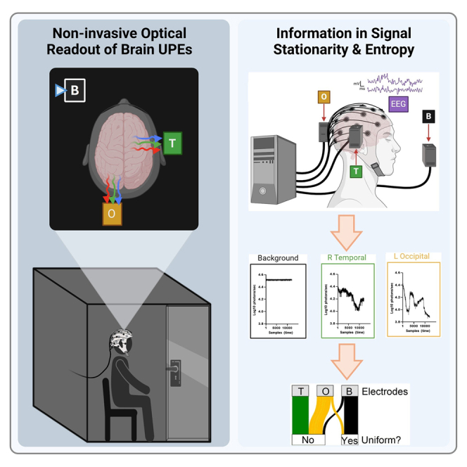
Graphical abstract

Highlights

• •Ultraweak photon emissions (UPEs) were detected in resting and active human brains
• •Brain UPE spectra and entropy vary by task, diverging from background levels
• •Optical readouts correlate with evoked neuroelectric oscillations across tasks
• •Label-free photoencephalography represents a novel method for brain monitoring

Cognitive neuroscience; Neuroscience

Introduction

Cells and tissues are traditionally understood to communicate through molecules and gene transcription. However, an emerging dimension of biophysical signaling is gaining attention. It is well established that cells and tissues can communicate via electrical signals, particularly in the brain and heart. Increasingly, evidence points to the role of light signals, in the form of ultraweak photon emissions (UPEs), as being physiologically relevant and potentially useful as indicators of both healthy and diseased states.^1,2 These UPEs were first described as “mitogenic radiation” by Alexander Gurwitsch in 1923, following his pioneering experiments that demonstrated that onion roots could stimulate growth in nearby conspecifics, even when separated by glass barriers, but not by quartz.³ Subsequent studies corroborated the involvement of endogenous ultraviolet (UV) light as the mediating factor for this growth induction,⁴ highlighting the potential role of biophotonic signals in cellular communication and development.

This phenomenon has since been replicated in diverse uni- and multicellular organisms,^5,6,7,8 and due in part to the development of technologies such as photomultiplier tubes (PMT), single-photon counters (SPC), and charge-coupled devices (CCD), much has been learned about UPEs. Indeed, biological tissues continuously emit very low intensity light (∼10⁻¹⁶ W/m², a few thousand photons per cm² per second)⁹ within the visible-to-near-visible spectral range (200–900 nm). UPEs are generated by radiative decay of excited molecules and reflect the metabolic states of cells, correlating with the production of reactive oxygen species (ROS).² Consistent with the periodicities of hormonal fluctuations and oxidative metabolism, UPEs display diurnal and seasonal variations^10,11,12 and are coupled to mitochondrial respiration, of which ROS is a primary byproduct.¹³ However, UPEs can also be evoked by ligand-receptor interactions¹⁴ or by recent exposures to external light sources,^15,16 suggesting both endogenous and delayed re-emission mechanisms. Notably, UPEs are distinct from blackbody radiation, which is orders of magnitude less intense, and bioluminescence, which is typically more intense but related to specific biochemical reactions (e.g., luciferase in fireflies, jellyfish).¹⁷ Despite these advances and an emerging science of UPEs as participants in cellular communication,^2,18 limited practical applications have been implemented to date.

Neural tissues have received special attention as a source of UPEs due to their excitable physiology, high metabolic load,^19,20 and marked sensitivity to light stimulation.^21,22,23 Indeed, the wavelengths of resting and glutamate-induced UPEs shift significantly as a function of aging^{24,25,26,27,28} and cognitive potential.²⁹ Several investigators have hypothesized and successfully modeled optical neurotransmission, suggesting a role of myelinated nerve fibers as waveguides for UPE-based communication channels in the brain.^30,31 Thus, in addition to synaptic transmission, gap junctions, and ephaptic couplings, there is evidence to indicate that brain tissues display photonic transmission as a signaling modality. That neural cells express a diversity of photoactive molecules, including non-visual opsins (e.g., OPN3 or “encephalopsin”), auto-fluorescent neurotransmitters (e.g., serotonin), and flavins (e.g., cryptochrome) suggests that UPEs may serve recondite functions that could be leveraged to develop label-free in vivo imaging techniques.³²

Current functional neuroimaging approaches use ionizing radiation (e.g., positron-emission tomography or PET), high-intensity magnetic fields (e.g., functional magnetic resonance imaging or fMRI), and near-infrared light (e.g., functional near-infrared spectroscopy or fNIRS) to resolve functional brain states. Although fNIRS and fMRI are relatively non-invasive compared to PET, brain tissues are highly responsive to magnetic fields³² as well as infrared and near-infrared wavelengths of light (650–950 nm), which can suppress or enhance neurotransmission^33,34,35,36 and neural oscillations,^37,38 thus complicating interpretations of functional readouts. Whereas many functional imaging techniques involve the application of activity-inducing stimulation by the instrument itself, some including electroencephalography (EEG) and magnetoencephalography (MEG) are fully passive.³⁹

Analogous to the passive measurement of microvolt fluctuations over the scalp associated with EEG, we hypothesized that passive measurement of brain UPEs would be maximally non-invasive and non-confounding. That is, since no external stimulus is applied, which might induce or suppress neural activity, imaging would be safe and unperturbed. Passive measurement would also enable the identification of relationships between ambient electromagnetic stimuli in the environment and brain activity. Further, because EEG profiles can be predictably altered without the use of optical stimuli, either by auditory stimulation or by simply closing one’s eyes (i.e., 10 Hz “alpha-generating”), UPEs may be measured simultaneously. Here, we sought to characterize UPE patterns detected from human brains while the participants engaged in tasks that are known to affect brain activity as measured by conventional neuroimaging devices such as quantitative EEG (qEEG). UPEs over the occipital and temporal lobes were distinguished from background measurements as a function of signal variability, entropy, and stationarity. Temporal dynamics of brain, but not background UPEs, also changed as a function of task, suggesting a potential application of passive brain light recordings. Some associations were identified between neural oscillations and brain UPEs; however, several parameters are discussed that should be considered when interpreting biological relevance, to optimize functional readouts, and to determine suitability for imaging applications or as a support of existing neuroimaging techniques.

Results

Brain UPE signals can be distinguished from the background signal

Although UPEs have been previously linked to brain functions,^26,40,41 it is yet to be determined whether human brain UPE signals can be distinguished from local background photon noise across several signal parameters. We investigated whether UPE recordings over the left occipital and right temporal lobes (five tasks, 2 min each as outlined in the STAR Methods section) exhibited a distinct signature compared to background UPE signals (Figure 1).

Figure 1.

qEEG and UPE recordings were collected simultaneously from human participants

(A) Participants sat quietly in a darkened chamber with PMTs positioned over regions of the head coinciding with qEEG electrodes over the left occipital (O) or right temporal (T) lobes. Background (B) UPEs were also recorded approximately 45 cm anterior and 15 cm lateral to the head, with the aperture directed toward an adjacent wall, away from the participant.

(B) Simultaneous recordings of PMT photon counts and EEG microvolt fluctuations were collected while the participant rested with their eyes open or closed, during periods of silence and exposures to repetitive auditory stimulation.

(C) Representative traces (Log10 photons/sec) for L Occipital (yellow), R Temporal (green), and Background (black) PMT recordings over the 10-min recording period are presented (horizontal axis: samples or time, implicitly). Images were created using BioRender.

As seen in Figure 2A, normalized UPE counts were plotted over time for each combination of subject and PMT (B: Background; O: Occipital; T: Temporal; Subject ID: 1:20). Using a hierarchical clustering approach, we computed the pairwise distances between PMTs for each subject (Figure 2B, left) as a proxy of UPE signal similarity. We hypothesized that brain signals (occipital and temporal) would exhibit more similar UPE temporal dynamics (lower pairwise distance) compared to background signals. Accordingly, the pairwise distance was significantly lower for the Occipital-Temporal (O-T) pair compared to either Background-Occipital (B-O) or Background-Temporal (B-T) pairs. We then computed the coefficients of variation (CVs; Figure 2B, central) and entropy values (Figure 2B, right) for each raw UPE trace as a proxy of signal variability and complexity, respectively. Both the Occipital and Temporal UPE signals showed increased signal variability (CV) and complexity (entropy) compared to Background UPE traces.

Figure 2.

Brain UPE signals possessed distinct temporal dynamic, increased variability, and complexity

(A) Normalized (red: max; green: min) UPE count over time. Each row represented a different UPE trace; the first letter (B, O, T) represented the type of PMT (Background, Occipital, Temporal; black, orange, green, respectively) and the number represented the subject ID. The dendrogram has been computed using correlation as distance metric and average as linkage method.

(B) Mean (square) and individual (gray circles) pairwise distance, CV and entropy computed using the entire UPE traces.

(C and D) Mean (square) and individual CV and entropy values within PMTs across task (top) or within task across PMTs (bottom). Mean ± SD. All asterisks indicate p < 0.001. Statistic: generalized linear mixed effect models. Black: Background; orange: Occipital; green: Temporal. All statistical statements can be found in Tables S1 and S2 of the Supplementary Files.

These results revealed that brain-derived UPE signals had a distinct temporal dynamic compared to background photon signals, exhibiting greater similarity to each other than when compared to local background signals and had increased entropic content and variability.

Entropy and UPE trace variability remain consistent across tasks and weakly distinguish between PMTs for a given task

We then investigated whether CV and entropy varied as a function of the task (Eyes Open pre, Eyes Closed pre, Music, Eyes Closed post, and Eyes Open post; pre and post refers to the Music task). CV and entropy (Figures 2C and 2D, respectively) are shown for each PMT across tasks or for each task across PMTs. For all the PMTs, both CV and entropy showed no significant changes across tasks (See Table S1). With few exceptions distinguishing between background and brain UPE signals, CV and entropy were not different between PMTs for a given task. These results showed that neither entropy nor CV changed across tasks within PMTs and that they only weakly distinguished between background vs. brain UPE signals for some tasks.

A distinct brain spectral frequency pattern, independent of specific tasks, distinguishes occipital UPE signals from background signals

Rhythmic activities are essential for brain function and have defined analytical approaches to understanding brain states associated with sleep, attention, memory, and other cognitive features.⁴² Therefore, we explored whether brain UPE signals exhibit distinct frequency patterns compared to background signals.

Representative spectrograms and averaged power spectra graphs for each PMT are shown in Figures 3A and 3B, respectively. After visual inspection of the averaged power spectra, we binned the frequency range into three bands: Band1 (0.1–0.3 Hz), Band2 (0.3–1 Hz), and Band3 (1–10 Hz). Since the power for each band did not significantly change neither over time nor across PMTs (Table S1), we averaged the power over time for each band and plotted it across PMTs (Figure 3C). The averaged power was significantly different between background and occipital UPE signals for both Band1 and Band2.

Figure 3.

Brain UPE possessed unique spectral signature below 1 Hz

(A) Representative spectrograms.

(B) Mean power spectra for each PMT (Background: black; Occipital: orange; Temporal: green).

(C) Mean (bar graph) and individual mean power values across bands for each condition (Band 1: 0.1–0.3 Hz; Band 2: 0.3–1 Hz; Band 3: 1–10 Hz).

(D) Similarity matrices analyzing the entire range of spectrogram’s frequencies, Band 1, Band 2, and Band 3, as indicated.

(E) Mean (square, black) and individual (circle, gray) MSE values for each pair of PMTs (B-O: Background-Occipital; B-T: Background-Temporal; O-T: Occipital-Temporal). Mean ± SD. All asterisks indicate p < 0.001. Statistic: generalized linear mixed effect models. Black: Background; orange: Occipital; green: Temporal. All statistical statements can be found in Tables S1 and S2 of the Supplementary Files.

Since the prior analysis averaged the UPE signals over time, we further investigated whether the inclusion of the UPE temporal dynamic confirmed a unique brain spectral pattern compared to the background. We used an imaging approach to quantify signal similarity across all pairwise combinations of UPE signal spectrograms (similarity was quantified using the MSE value; see STAR Methods). In Figure 3D, the similarity matrices for the entire UPE spectrograms and each individual band are shown. The pairwise normalized MSE values summarized in Figure 3E confirmed that the spectrograms of occipital and temporal UPE signals are more similar to each other below 1 Hz (lower MSE values; Band1 and Band2) compared to the background UPE spectrograms. While analyzing Band3, the brain UPE spectral signature was indistinguishable from background. These results showed that the brain UPE signals had a distinctive frequency signature in the range 0.1–1 Hz, implying rhythmic emission patterns or bursts ranging from once every 10 s to once every second.

Brain UPE signals exhibit discrete stationary counts changing across task

After having examined the temporal changes in UPE signals, we tested the hypothesis that different brain states are associated with defined and stable UPE counts. We proposed that, if the brain state remains stable (the same task is prolonged in time) and enough time is allowed (considering that UPE operate on slower time scales than electrical activities), UPE counts reach a stationary state. Accordingly, changes in UPE signals can only be detected during task transitions. If the hypothesis was correct, the implications included, but were not limited to, achieving a stationary signal and observing task-dependent changes in brain-derived UPE signals, as different tasks correspond to different brain states. Therefore, we tested the hypothesis that, by the end of each 2-minute-long task, a stationary UPE count is reached and that this count varies specifically between eyes open/closed tasks in the brain signals.

Representative UPE trace (black) with the last 10 s (arbitrary time stretch; small enough to test robustly for stationarity and long enough to be potentially of biological relevance) for each task highlighted (blue) and magnified are shown in Figure 4A. To determine whether a stationary UPE count is reached at the end of each task, we first computed the deviation of each UPE count from its median for each 10-s segment (Deviation, Figure 4B). Segments were classified as stationary if their median deviation was lower than 0.015 (see STAR Methods), indicating that the median deviation of the UPE segment from its median value was lower than 1.5% (Figure 4B, green trace). We formulated the stringent null hypothesis that, by chance, only 5% of the segments are not stationary under the assumption of a stationary UPE count at the end of each task. We then determined the fraction of stationary vs. non-stationary segments for each PMT and compared it to null hypothesis. All PMTs showed a stationary UPE signal in the last 10 s of each task (Figure 4B).

Figure 4.

UPE signals reached a stationary signal at the end of each task and only the brain UPE traces showed task-to-task changes

(A) Representative UPE raw counts for the entire trace (black) or the last 10 s at the end of each task (blue).

(B) Left: workflow to classify the segments as stationary (green) or non-stationary (red). Right: percentage of stationary vs. non-stationary segments across null hypothesis and each PMT.

(C) Alluvial plot (top) and representative traces (bottom) illustrating the changes in the following categorical variables: segment was uniform (yes/no), the relative count between EO (blue line) and EC (red line) tasks changed or not after the music task. Among the possible trends (relative change between EO and EC before and after music), seven combinations of raw UPE counts were found (from top to bottom): EO < EC before and after music, EO > EC before and after music, EO = EC before and EO > EC after music, EO = EC before and EO < EC after music, EO < EC before and EO > EC after music, EO > EC before and EO = EC after music, EO > EC before and EO < EC after music.

(D) Mean (square, black) and individual (circle, gray) normalized UPE changes in the EO/EC conditions before and after music across PMTs. Green shaded area and red shaded area delimited the points that were considered variable (namely, the change was greater than 0.009) or uniform, respectively.

(E) Top: percentage of uniform/variable segments across null hypothesis and each PMT. Bottom: percentage of affected/not affected relative UPE counts before and after music across null hypothesis and each PMT. Mean ± SD. Statistic: generalized linear mixed effect models. Black: Background; orange: Occipital; green: Temporal.

We then examined whether the relative UPE stationary counts varied between Eyes Open (EO) and Eyes Closed (EC) tasks, based on the hypothesis that brain UPE counts may reflect distinctions between these two brain states. While the tasks included an auditory stimulus (music), we analyzed the relative UPE count changes only across EC and EO tasks. In fact, unlike M, EC and EO tasks have well-established and robust distinct brain signatures. The alluvial plot in Figure 4C summarized the fraction and type of UPE signals that were considered uniformed or variable (Yes and No, respectively), changed the EO/EC relative count before and after Music and their specific trends. Representative traces for each condition are shown in Figure 4C. For each EO/EC pair before and after the Music task, we computed the normalized UPE change (Figure 4D; see STAR Methods). We classified a UPE signal as variable (green shaded area) if the EO/EC change either before or after Music exceeded 0.009 (three times higher than the median change in the background signal); otherwise, it was considered uniform (red shaded area). Figure 4E (top) showed the percentage of UPE traces classified as uniform across PMTs. We formulated the stringent null hypothesis that the traces were not uniform by chance (5%), under the assumption that brain UPE counts vary between EO and EC tasks. The background condition, but not the brain signals, violated the null hypothesis.

We finally examined whether exposure to the auditory stimulus affected the relative UPE count between EO and EC tasks (Figure 4E, bottom). All conditions failed to reject the flat null hypothesis that M had an equal chance to change or not the trend. The results demonstrated that a stationary signal is achieved, and significant variations across tasks were observed exclusively in brain UPE signals. However, the direction of these changes was not consistent among subjects before and after the M task.

Brain spectral power displays condition-dependent correlations with UPE measures

Upon examination of the qEEG data (n = 20), we identified two (n = 2) participants with significant electrical artifacts within their records, thus preventing spectral power density (SPD) extractions across some tasks. Both participants were excluded from analyses involving qEEG data.

To determine whether brain rhythms associated with lobes proximal to PMTs were affected by tasks, we examined averaged SPDs (μV² Hz⁻¹). As expected, alpha (7.5–14 Hz) SPDs increased over both the left and right occipital lobes (O1 and O2 sensors, respectively) when participants’ eyes were closed (EC) relative to when they were open (EO) (Figure S1A). The EC condition also produced increased theta (4–7.5 Hz) SPDs and decreased beta 1 (14–20 Hz) SPDs when compared to EO. Delta and gamma rhythms were not impacted by EC-EO conditions. These results confirmed that brain rhythms were reliably affected by closing one’s eyes in a relaxed state and provided context for task-dependent UPE changes reported elsewhere.

We then tested the hypothesis that occipital UPE counts and alpha-band SPDs vary systematically. Performing simple linear regression, during the EO condition, there were no discernable relationships between UPEs and SPDs. However, when the participants closed their eyes (EC condition), both background and occipital UPEs (averaged over the EC condition period) correlated with alpha-band SPDs over the occipital lobes (Figure 5A). There was no discernable relationship between temporal UPEs and alpha SPDs from the occipital regions.

Figure 5.

Brain SPDs display condition-dependent correlations with UPE measures

(A) Average photon (UPE) counts for background (Backg., gray), occipital (Occ., orange) and temporal (Temp., green) PMTs plotted with left occipital (L Occ.) alpha (7.5–14 Hz) spectral power densities (SPD) during the eyes open (EO) and eyes closed (EC) conditions.

(B) Coefficient of variation (CV) of UPE counts for Backg., Occ., and Temp. PMTs plotted with left (L) and right (R) temporal (Temp.) alpha SPDs during the Music condition, where a 120 BPM auditory stimulus was presented to the right side of the participant, outside the darkened chamber.

(C) Average UPE counts over the left occipital PMT plotted with right temporal (R Temp.) SPDs within the delta (1.5–4 Hz), theta (4–7.5 Hz), alpha (7.5–14 Hz), beta 1 (14–20 Hz), beta 2 (20–30 Hz), and gamma (30–40 Hz) band ranges during the Music condition. Spearman rho (ρ) values and significance (∗ = p < 0.05) are reported for each plot. All statistical statements can be found in Table S2.

Next, we sought to determine whether SPDs over the temporal lobes were affected by the 120 BPM auditory stimulus (M condition). As expected, due to the right-sided presentation of the stimulus, high-frequency activity across beta 1 (14–20 Hz), beta 2 (20–30 Hz), and gamma (30–40 Hz) spectral bands decreased significantly over the left temporal lobe (contralateral to the stimulus) during the M condition (Figure S1B). Lower frequency (1–7.5 Hz) SPDs within the left temporal lobe was not affected by exposure to an auditory stimulus. Right temporal lobe SPDs were not affected by auditory stimulation across all bands (delta-gamma). Then, we tested the hypothesis that high-frequency SPDs over the temporal lobes would correlate with average UPE counts over the same region during the M condition, though no relationship could be discerned. However, a relationship between right temporal beta 2 SPDs and occipital UPE counts was identified, which was not evident at any other frequency band (Figure 5C). There was no relationship between background photon counts and temporal lobe SPDs. Interestingly, during the M exposure, temporal and occipital UPE variability (CV) correlated with alpha SPDs over the left temporal lobe (Figure 5B). Only occipital UPE variability correlated with alpha SPDs over the right temporal lobe. Background photon variability did not correlate with any temporal lobe brain rhythms during auditory exposures.

Together, these data indicate that although UPE and SPDs may vary together during tasks that change SPDs, and relationships tend to be within expected frequency bands associated with task-dependent SPD changes, there are unexpected effects across qEEG-PMT proximal sensor pairs.

Discussion

As the first proof-of-concept demonstration that UPEs from human brains can serve as readouts to track functional states, we measured and characterized photon counts over the heads of participants while they rested or engaged in an auditory perception task. We demonstrated that brain-derived UPE signals can be distinguished from background photon measures. Additionally, our results suggest that for a given task, the UPE count may reach a stable value (steady state). The data indicated that the primary distinguishing factor between brain vs. background UPE signals was the variation in raw count of brain UPE traces across different tasks. This variation was reflected in the increased variability and information content (Figure 2). Additionally, these changes occurred at frequencies below 1 Hz (Figure 3), suggesting a different rate of change between electrical (qEEG) and UPE signals. Indeed, we predict that fast brain state shifts might not be reflected in the UPE trace dynamics. If metabolically driven UPE fluctuations and electric field oscillations operate at different scales of time, there will be a need to identify the relevant transform that enables an analysis of mutual information or shared variances.

On the basis of our initial observations, we proposed and began to explore a novel hypothesis: UPE counts are stationary for a long-enough task (Figure 4). Although this suggests a relationship between UPE counts and electrical oscillations in the brain, our current dataset only supported a limited analysis of their potential connection (n = 18). Nevertheless, we did identify correlations between UPEs and qEEG spectral power (Figure 5), motivating future investigations with higher density sensor arrays. However, future investigations should involve larger sample sizes and designs incorporating distinct tasks that generate unique qEEG profiles. With the ability to synchronize PMT and qEEG recordings at the millisecond scale, there is the potential to observe UPE dynamics during highly stereotyped event-related potentials (ERPs). However, it remains uncertain whether strong correlations between neural oscillations and UPEs should be anticipated, given their different generative mechanisms and timescales. Brain UPEs may also be differentially expressed by inhibitory or excitatory neurons as well as by glial cells, which serve complex metabolic functions. If circum-cerebral UPEs reflect the brain’s regional metabolic load, they may also reflect individual differences of functional connectivity and other factors. Alternatively, a variation in the rate of change of the UPE signals could suggest that various brain regions achieve a steady state at different times.

It was originally assumed that UPE dynamics would differ as a function of whether the participants’ eyes were open or closed, reflecting the well-documented effects on alpha rhythms associated with this standard neuroimaging task using electroencephalography. Given that neural oscillations within the alpha band are reliably modulated by the presence or absence of visual stimuli, we predicted that similar changes in UPEs would be detected with increased metabolic activity among active cell populations—particularly within the occipital lobe. We did observe brain UPE count differences as a function of whether participants’ eyes were open or closed (Figure 4E). However, the relative change in counts between these tasks varied among subjects, possibly indicating that either the tasks alone did not fully explain the direction of UPE change or the direction of UPE change was weakly linked to the task. There may be a temporal disconnect between UPE-generative mechanisms and those that underlie neural oscillations that could account for this unanticipated finding.

Interestingly, background photon counts and occipital alpha SPDs correlated when participants’ eyes were open (Figure 5A). It may be relevant that, in previous studies, alpha rhythms over the occipital lobe were found to correlate with ambient magnetic field fluctuations in real time^43,44,45 and could be attenuated by magnetic shielding and rescued by exposures to artificially generated simulations of Earth’s magnetic field.⁴⁶ We have previously highlighted that alpha rhythms may be, in part, driven by exogenous stimuli.³² In the present study, we determined that when participants closed their eyes, background photons and UPEs over the occipital lobe varied systematically with occipital alpha rhythms. Temporal UPEs, while displaying dynamics that were similar to occipital UPEs and distinct from background photons, did not correlate with brain SPDs. Together, these data support a potential connection between brain rhythms, UPEs, and ambient electromagnetic conditions; however, further experiments with shielding conditions are needed to make conclusive statements.

As brain UPE detection technologies continue to develop, it will be important to consider several factors to optimize their predictive power. For example, UPE wavelengths were not considered in the current study but were previously found to be predictive of aging,^24,25,27,28 cognitive potential,²⁹ as well as essential discriminants of healthy and diseased states.^47,48 Our PMTs were calibrated to detect a wide band of UPE wavelengths, which was intentionally inclusive but may have obscured or diluted narrow-band effects. Thus, the use of filters or tunable photodetectors is recommended to determine the wavelength dependencies of brain UPE pattern signatures. Similarly, the present study involved the use of limited sensor array over a few regions of interest. To better understand how brain UPE patterns are related to connectomes and enable deep-tissue source localization, it will be necessary to use higher density arrays of photodetectors that will greatly improve the spatial resolution of the technique. Unlike electric field oscillations, which when detected by qEEG reflect nearby cell activations (likely within the first few millimeters of cerebral cortex), UPEs detected over the surface of the head could originate from many radiative point sources within the cerebrum—particularly from superficial regions where expected attenuation is not as extreme. This could explain why we observed a relationship between left occipital UPEs and high-frequency oscillations within the right temporal lobe (Figure 5C). Because UPEs are generated by molecular reactions, the number of potential point sources for emissions far exceeds the number of cells within the system. Although this may complicate source localization, we would suggest that a combination of detector arrays and machine learning tools could enable engineers to re-construct UPE dynamics in three-dimensional space for neuroimaging applications—particularly if UPE point sources are spatially clustered rather than homogenously distributed. Because UPEs are related to oxidative metabolism, the most immediately relevant applications might include the detection of budding brain tumors, excitotoxic lesions, mild traumatic injuries, and neurotoxic insults (e.g., chemobrain).

Toward engineering a “photoencephalography” technique with which to infer functional brain activations on the bases of endogenous light emissions coupled to oxidative metabolism from neural tissues, additional experiments are needed to isolate key signal parameters. One of the major challenges that must be overcome before brain UPE measurements become a practical reality for clinical applications is the identification of fingerprint-like patterns akin to ERPs and other stereotypical features. However, just as MEG measurements reveal femtoTesla-scale (10⁻¹⁴ T) magnetic field fluctuations that are predictive of brain states despite microTesla-scale (10⁻⁶ T) ambient magnetic noise (100 million times more intense), we view the current results as a proof-of-concept demonstration that patterns of human-brain-derived UPE signals can be discriminated from background light signals in darkened settings despite very low relative signal intensity. Photoencephalography would be maximally non-invasive (i.e., passive recording) with high temporal resolution, like EEG or MEG; however, the measurement of UPEs would be linked to oxidative metabolism with several clinical applications described elsewhere. Future studies may find success in using select filters and amplifiers to sieve and enhance UPE signal features from healthy and diseased brains.

Limitations of the study

One limitation of the study was a lack of simultaneous non-brain tissue PMT measurements to differentiate UPE generators by metabolic load, ROS production, heat production, electrical excitability, and other physiological features. Similar to the inclusion of multiple PMTs to source-localize UPEs in the brain, additional PMTs across the body may help disentangle unanswered questions about the relationships between UPEs and systemic physiology. Future studies should incorporate measurements from limbs, digits, and other organs (e.g., liver, heart) that may display unique, tissue-dependent signal properties. If signals can be discriminated with UPE signals alone, there may be several biomedical applications that go beyond neuroimaging. Although the sample did include similar proportions of self-identified men and women, it should be noted that the small sample limited a detailed exploration of gender- or sex-based differences. Future studies should aim to identify unique UPE signatures reflective of known metabolic and neuroanatomical differences across these groups.

Resource availability

Lead contact

Further information and requests for resources, data, and codes should be directed to and will be fulfilled by the lead contact, Dr. Nirosha J. Murugan (nmurugan@wlu.ca).

Materials availability

All materials and methods are presented in the paper, are available on Zenodo (https://zenodo.org/records/13903556), or can be made available upon request from the lead contact.

Data and code availability

• •Data: all data are presented in the manuscript and can be accessed upon request from the lead contact.
• •Code: standard MATLAB code was used for analysis, all of which can be found explicitly named under the quantification and statistical analysis section. For each panel, the model, dataset, and modeling parameters are available on Zenodo (https://zenodo.org/records/13903556).
• •Additional information: any additional information that is required to analyze the data reported in the paper can be obtained by contacting the lead contact.

Acknowledgments

The authors acknowledge support from the National Sciences and Engineering Council of Canada (NSERC), Discovery Grant RGPIN-2021-03783 (to N.J.M.), as well as the New Frontiers in Research – Exploration Program, Grant NFRFE-2020-01351 (to N.J.M.), and the Optica Foundation. N.R. and N.M. acknowledge support from the Allen Discovery Center at Tufts University.

Author contributions

Study conception and design, N.M. and N.R.; data collection, H.C. and I.D.; data processing and management, H.C., I.D., and M.B.; analysis and interpretation of results, N.M., M.B., and N.R.; draft manuscript preparation, N.M., M.B., and N.R.; revisions, N.M., N.R., and M.B. All authors reviewed and approved the final version of the manuscript.

Declaration of interests

The authors report no conflicts of interest, financial or otherwise.

STAR★Methods

Key resources table

REAGENT or RESOURCE	SOURCE	IDENTIFIER
Software and algorithms
MATLAB	MathWorks, Inc.	Version 2023b
Standardard MATLAB Code	Zonodo (archived)	https://zenodo.org/records/13903556 https://doi.org/10.5281/zenodo.13903556
Windows 10 OS	Microsoft	20H2
Counter Timer Software	Sens-Tech	Version 2.8, Build: 11
WinEEG Software for Mitsar	Bio-Medical, Inc.	#NTE WINEEGADV
Other
Mitsar-202 QEEG amplifier	Bio-Medical, Inc.	#NTE MITSAR20224
19-Channel Electro-Caps	Bio-Medical, Inc.	#ECA CAPS
Electro-gel for Electro-Caps	Bio-Medical, Inc.	#ECA E9
BD Luer-Lok Tip Syringes - 5mL	Bio-Medical, Inc.	#ECA E7B-5ML
Electro-Cap Tin Ear Electrodes - 9mm	Bio-Medical, Inc.	#ECA E5-9S
Photomultiplier Tubes	Sens-Tech	DM0090C
Gooseneck Mount/Clamp	Lamicall	LS05-CA-B
Smartphone	Google	Pixel 7 (GVU6C, GQML3)
Laptop Computer	DELL	Inspiron 15 (7000)

Experimental model and study participant details

Participants

A total of twenty (n=20) adults were recruited with publicly displayed advertisement and consented to the participate in the study. The sample consisted of 10 women, 9 men, and 1 non-binary individual, with a mean age of 25.4 years (range: 19–52) (see Table S3 for demographics details). All participants were naïve to the purpose of the experiment and were asked to follow basic instructions while sitting in a darkened room. All participants had normal or corrected-to-normal vision and reported no history of mental health problems or neurological disorders. Participants were not allocated to specific groups because of the within-subject experimental design (i.e., all participants receive the same exposure conditions). Written informed consent was obtained from all of the participants. All study procedures were conducted after approval from the institutional Research Ethics Board at Algoma University (Study Approval Number: 026-202122).

Method details

Measurement chamber

The study involved the simultaneous measurement of scalp surface potentials and UPEs over the participant’s head during a 10-min recording period. Before initiating the recordings, participants were guided to a darkened room, which comprised of a small chamber (2.2 m x 1.5 m) within a larger darkened laboratory space and sat in a comfortable, padded chair. qEEG and PMT devices were positioned on or around the head as described elsewhere. The enclosed chamber was darkened with black wall coverings and the external laboratory space was devoid of all light sources with the exception of laptops used for qEEG and PMT recordings, which were set to minimum brightness settings. Cables connecting computers in the outer laboratory space and sensors in the chamber passed through small holes located at the bottom of the chamber wall behind the participants.

General procedure

Following a brief description of the procedures, darkening the room, and uncovering PMTs, the recording were initiated and carried out in the following order: (1) 2 mins of baseline recordings with the participants’ eyes open (EO-Pre), (2) 2 mins of baseline recordings with the participants’ eyes closed (EC-Pre), (3) 2 mins continuous exposure to an auditory stimulus (M), (4) 2 mins of baseline recordings with participants’ eyes closed (EC-Post), (5) 2 mins of baseline recordings with participants’ eyes open (EO-Post). After the recording procedure, PMTs were covered, lights were turned on, the EEG cap was removed, and the participant was debriefed. Data were always collected during the daytime, between 9:00 and 18:00 EST.

Auditory stimulus

An auditory stimulus consisting of a repeating (120 bpm, 2 Hz) click with a woody “block” timbre and spectral peak of 921 Hz was delivered via a Google Pixel 7 smartphone, placed outside of the darkened chamber. The stimulus was always delivered without warning to the right side of the body at the 4-min time point of the experimental procedure when participants’ eyes were closed, and individuals were later asked to confirm the audible sounds after the full, 10-min recording period. For the purposes of labelling only, conditions involving the auditory stimulus will be referred to as “music” or “M” throughout the analysis. Similar auditory stimuli were previously found to affect high-frequency brain rhythms.^49,50

Ultraweak photon emissions (UPEs)

Photomultiplier tubes (PMTs) (Sens-Tech DM0090C) were positioned around the participants to record photon counts (s-1) indicative of ultraweak photon emissions (UPEs). Each device contained a 22-mm S20 cathode, displayed a spectral range of 300-850 nm, and was rated for typical dark counts of ∼1000s-1. Devices logged data via a USB connections to DELL laptops running Windows 10 OS and powered by an external 9V AC supply (input voltage was ∼5V).

Two PMTs were positioned approximately 5 cm over the surface of the head with their apertures facing corresponding brain regions of interest, including the left occipital lobe (PMT-O) and right temporal lobe (PMT-T). The PMT-O aperture was always facing the head and positioned medial to the O1 sensor of the qEEG cap, while the PMT-T aperture was always positioned slightly ventral relative to the T4 sensor of the qEEG cap (19-channel ECI Electro-Cap). A third PMT was placed approximately 30 cm anterior and 10 cm lateral to the participant on their left side, with its aperture pointed toward a wall, away from the door. Standard measurement parameters were set within the Sens-Tech Counter Timer Software, including high-cut (30 Hz), notch-filter (60-120 Hz), and gain (100 μV). The period of recording was set to 40 ms (25 Hz) for a total of 15,000 measurements within 10 minutes. Devices were only uncovered while in darkened environments, with a 5-min buffer between exposing apertures and initiating recordings.

Quantitative electroencephalography (qEEG)

Microvolt (μV) fluctuations over the surface of the scalp were measured with a quantitative electroencephalography (qEEG) system (Mitsar-202 amplifier) connected to a DELL laptop running WinEEG software on a Windows 11 OS. Each participant wore a 19-channel cap with sensors distributed according to the 10-20 international system (19-channel ECI Electro-Caps). A monopolar montage was used, referenced to two electrodes attached to participants’ ears. Impedance values of less than 5 kOhm were always achieved before initiating recordings. Measurements were collected at a sample rate of 250 Hz, with 100 μV gain and applied low-cut and high-cut filters of 1.6 Hz and 50 Hz, respectively. Notch-filters of 50-70 Hz and 110-130 Hz were also applied. Spectral densities (μV2 Hz-1 or SPDs) were extracted from WinEEG from 30 second segments of raw data, yielding 4 extracts per 2-minute condition. Default band ranges were defined as the following in WinEEG: delta (1.5Hz-4Hz), theta (4Hz-7.5Hz), alpha (7.5Hz-14Hz), beta1 (14Hz-20Hz), beta2 (20Hz-30Hz), and gamma (30Hz-40Hz). Before analysis was performed, several averaged variables were computed, including averaged SPDs over the full task period, and lobe- and/or hemisphere-specific aggregates (e.g., right temporal lobe: SPD averages of T4 and T6 sensors).

Quantification and statistical analysis

Hierarchical clustering analysis

Raw UPE count signals had been used as input of the clustergram.mat function, using correlation as a distance metrics (to compare patterns rather than absolute values) and average as linkage method (balanced approach less sensitive to outliers). Pairwise distances have been extracted after computing the distance matrix using pdist.mat function followed by squareform.mat function.

Entropy and coefficient of variation

Shannon’s entropy of UPE signals have been computed accordingly to:

$$H\left(X\right)=-\sum _{x\in X}p\left(x\right)·{\log }_{2}p\left(x\right)$$

where $H\left(X\right)$ is the entropy of the variable $X$, $p\left(x\right)$ is the probability of the $x^{th}$ event occurring, $p\left(x\right)·{\log }_{2}p\left(x\right)$ represents the information content of the $x^{th}$ event weighted by its probability. $p\left(x\right)$ has been computed dividing the vector of the histcounts.mat function by its sum, using either the entire trace or each task as input. The number of bins for the histcounts.mat function has been selected by using the Freedman-Diaconis rule, ensuring that the histogram provided an informative representation of the data’s distribution. Briefly:

$$bins=\frac{range}{binwidth}=ceil\frac{(\max \left(x\right)-\min \left(x\right))·\sqrt[3]{n}}{2·IQR}$$

where $(\max \left(x\right)-\min \left(x\right)$ is the range of the distribution, $n$ is the total number of points in the distribution, $IQR$ is the interquartile range. The optimal number of bins has been selected as the median bin numbers across all traces and PMTs, resulting in 49 and 35 bins for the entire trace or for each two-minutes-long task, respectively.

Coefficient of variation (CV) has been computed as the ratio between the standard deviation and the average of the entire trace or within task.

Short-time Fourier transform

The short-time Fourier transform (STFT) has been used to analyze the frequency content of nonstationary UPE signals over time. stft.mat function has been used with a time window of 20 seconds and a fraction of overlap between two consecutive windows of 75%; the spectral leakage has been reduced using Hanning window. The spectrogram has been reconstructing by plotting the power (in dB) over time at each frequency. Considering the frequency of acquisition of UPE signals of 20 Hz and the time window of 20 seconds, the frequency range was analyzed between 0.1 Hz (twice the smallest analyzable frequency of 0.05 Hz) and 10Hz (half the frequency of acquisition).

For each frequency band (Band1: 0.1-0.3 Hz; Band2: 0.3-1 Hz; Band 3: >1 Hz), mean power has been computed across the entire trace within the frequency band range.

To quantify and compare the similarity of the spectrograms, hence considering their temporal dynamic, we applied the immse.mat function, a metric to quantify the pixel-by-pixel similarity between two images (spectrograms). Briefly, the mean-squared error (MSE) is computed for each pairwise combination of spectrograms, whether lower values indicate greater similarities. The resulting similarity square matrix was then used to perform a hierarchical clustering analysis. We performed the analysis of the entire spectrogram, of the spectrogram with frequencies lower than 1 Hz (due to the low number of points in Band1 and the inability to perform the immse.mat function, the Band1 and Band2 were merged) or grater than 1 Hz (Band3).

Signal stationarity

After extracting the last ten seconds of UPE raw counts for each task across PMTs, each trace has been filtered by calculating the moving average using movmean.mat function, with a window of 10 points (500ms). Subsequently, we calculated the median value for each filtered segment and used it to determine the deviation, defined as the absolute difference between the filtered segment and its median, divided by the median itself. The median of the resulting deviation values was then compared to an arbitrary threshold of 0.015. This threshold corresponds to a median deviation of 1.5% from the median value of the trace. If the median of the dispersion values was less than 0.015, the segment was classified as stationary; otherwise, it was considered non-stationary.

To determine if the stationary signal varied between eyes closed/open tasks, we computed the averaged values of the last ten seconds for each task and normalized by the average UPE count of the first task (Eyes Open, Pre Music) within subject. Based on median change (computed as the absolute difference between eyes open vs closed task before and after music) of 0.003 in the background signal (under the assumption that the background UPE should not vary in a task-dependent manner), we classified the UPE stationary signal as variable if the change either before or after music was greater than 0.009 (three times greater than the median change in the background signal); otherwise, it was considered uniform.

Statistical syntax

Unless otherwise indicated, statistical analysis has been conducted using generalized linear mixed-effect models (glme) in MATLAB, particularly to account for the nested structure and repetitive nature of the experimental design. For each model, the distribution (Normal, Gamma, Inverse Gaussian) and fit method (REMPL, MPL) have been selected by choosing the model maximizing the relative likelihood (i.e., ${\mathcal{L}}_T=e^{0.5·\left({AIC}_{\mathit{min}}-{AIC}_i\right)}$, where ${AIC}_{\mathit{min}}$ is the minimum AIC across all models and ${AIC}_i$ is the AIC for the ith model) and visual analysis of the residual. Chi-square proportional test results have been calculated after creating a contingency table and using it as an input for the crosstab.mat function. Post-hoc analysis has been performed using Bonferroni’s correction with alpha=0.05. For paired samples, the effect size has been computed as $d=\frac{D}{s_D}$, where $D$ is the averaged difference between paired samples ($D=\frac{\sum _{i=1}^n\left(x_n-y_n\right)}{n}$, where $n$ is the number of paired measures, $x$ is group 1 and $y$ is group 2) and $s_D$ is the standard deviation of $D$. For each panel, the dependent and independent variables, and statistical details (F-Statistic, degrees of freedom, p-values) have been summarized in Table S1.

Published: February 12, 2025

References

- 1.Du J., Deng T., Cao B., Wang Z., Yang M., Han J. The application and trend of ultra-weak photon emission in biology and medicine. Front. Chem. 2023;11 doi: 10.3389/fchem.2023.1140128. [DOI] [PMC free article] [PubMed] [Google Scholar]
- 2.Mould R.R., Mackenzie A.M., Kalampouka I., Nunn A.V.W., Thomas E.L., Bell J.D., Botchway S.W. Ultra weak photon emission—a brief review. Front. Physiol. 2024;15 doi: 10.3389/fphys.2024.1348915. [DOI] [PMC free article] [PubMed] [Google Scholar]
- 3.Gurwitsch A.A. A historical review of the problem of mitogenetic radiation. Experientia. 1988;44:545–550. doi: 10.1007/BF01953301. [DOI] [PubMed] [Google Scholar]
- 4.Hollaender A., Schoeffel E. Mitogenetic rays. Q. Rev. Biol. 1931;6:215–222. doi: 10.1086/394378. [DOI] [Google Scholar]
- 5.Berke J., Gulyás I., Bognár Z., Berke D., Enyedi A., Kozma-Bognár V., Mauchart P., Nagy B., Várnagy Á., Kovács K., et al. Unique algorithm for the evaluation of embryo photon emission and viability. Sci. Rep. 2024;14 doi: 10.1038/s41598-024-61100-8. [DOI] [PMC free article] [PubMed] [Google Scholar]
- 6.Fels D. Cellular communication through light. PLoS One. 2009;4 doi: 10.1371/journal.pone.0005086. [DOI] [PMC free article] [PubMed] [Google Scholar]
- 7.Sekulska-Nalewajko J., Gocławski J., Korzeniewska E., Kiełbasa P., Dróżdż T. The verification of hen egg types by the classification of ultra-weak photon emission data. Expert Syst. Appl. 2024;238 doi: 10.1016/j.eswa.2023.122130. [DOI] [Google Scholar]
- 8.VanWijk R. Bio-photons and bio-communication. J. Sci. Explor. 2001;15:183–197. [Google Scholar]
- 9.Calcerrada M., Garcia-Ruiz C. Human ultraweak photon emission: key analytical aspects, results and future trends–a review. Crit. Rev. Anal. Chem. 2019;49:368–381. doi: 10.1080/10408347.2018.1534199. [DOI] [PubMed] [Google Scholar]
- 10.Jung H.H., Yang J.M., Woo W.M., Choi C., Yang J.S., Soh K.S. Year-long biophoton measurements: normalized frequency count analysis and seasonal dependency. J. Photochem. Photobiol., B. 2005;78:149–154. doi: 10.1016/j.jphotobiol.2004.08.002. [DOI] [PubMed] [Google Scholar]
- 11.Kobayashi M., Takeda M., Sato T., Yamazaki Y., Kaneko K., Ito K., Kato H., Inaba H., Inaba H. In vivo imaging of spontaneous ultraweak photon emission from a rat’s brain correlated with cerebral energy metabolism and oxidative stress. Neurosci. Res. 1999;34:103–113. doi: 10.1016/s0168-0102(99)00040-1. [DOI] [PubMed] [Google Scholar]
- 12.Wijk E.P.A.V., Wijk R.V. Multi-site recording and spectral analysis of spontaneous photon emission from human body. Complement. Med. Res. 2005;12:96–106. doi: 10.1159/000083935. [DOI] [PubMed] [Google Scholar]
- 13.Pospíšil P., Prasad A., Rác M. Role of reactive oxygen species in ultra-weak photon emission in biological systems. J. Photochem. Photobiol., B. 2014;139:11–23. doi: 10.1016/j.jphotobiol.2014.02.008. [DOI] [PubMed] [Google Scholar]
- 14.Cifra M., Pospíšil P. Ultra-weak photon emission from biological samples: definition, mechanisms, properties, detection and applications. J. Photochem. Photobiol., B. 2014;139:2–10. doi: 10.1016/j.jphotobiol.2014.02.009. [DOI] [PubMed] [Google Scholar]
- 15.Bajpai R.P. Coherent nature of the radiation emitted in delayed luminescence of leaves. J. Theor. Biol. 1999;198:287–299. doi: 10.1006/jtbi.1999.0899. [DOI] [PubMed] [Google Scholar]
- 16.Cifra M., Brouder C., Nerudová M., Kučera O. Biophotons, coherence and photocount statistics: A critical review. J. Lumin. 2015;164:38–51. doi: 10.1016/j.jlumin.2015.03.020. [DOI] [Google Scholar]
- 17.Zapata F., Pastor-Ruiz V., Ortega-Ojeda F., Montalvo G., Ruiz-Zolle A.V., García-Ruiz C. Human ultra-weak photon emission as non-invasive spectroscopic tool for diagnosis of internal states–A review. J. Photochem. Photobiol., B. 2021;216 doi: 10.1016/j.jphotobiol.2021.112141. [DOI] [PubMed] [Google Scholar]
- 18.Sun Y., Wang C., Dai J. Biophotons as neural communication signals demonstrated by in situ biophoton autography. Photochem. Photobiol. Sci. 2010;9:315–322. doi: 10.1039/b9pp00125e. [DOI] [PubMed] [Google Scholar]
- 19.Benton D., Parker P.Y., Donohoe R.T. The supply of glucose to the brain and cognitive functioning. J. Biosoc. Sci. 1996;28:463–479. doi: 10.1017/s0021932000022537. [DOI] [PubMed] [Google Scholar]
- 20.Dienel G.A. Brain glucose metabolism: integration of energetics with function. Physiol. Rev. 2019;99:949–1045. doi: 10.1152/physrev.00062.2017. [DOI] [PubMed] [Google Scholar]
- 21.Ait Ouares K., Beurrier C., Canepari M., Laverne G., Kuczewski N. Opto nongenetics inhibition of neuronal firing. Eur. J. Neurosci. 2019;49:6–26. doi: 10.1111/ejn.14251. [DOI] [PubMed] [Google Scholar]
- 22.Blackshaw S., Snyder S.H. Encephalopsin: a novel mammalian extraretinal opsin discretely localized in the brain. J. Neurosci. 1999;19:3681–3690. doi: 10.1523/JNEUROSCI.19-10-03681.1999. [DOI] [PMC free article] [PubMed] [Google Scholar]
- 23.Sugihara T., Nagata T., Mason B., Koyanagi M., Terakita A. Absorption characteristics of vertebrate non-visual opsin, Opn3. PLoS One. 2016;11 doi: 10.1371/journal.pone.0161215. [DOI] [PMC free article] [PubMed] [Google Scholar]
- 24.Chen L., Wang Z., Dai J. Spectral blueshift of biophotonic activity and transmission in the ageing mouse brain. Brain Res. 2020;1749 doi: 10.1016/j.brainres.2020.147133. [DOI] [PubMed] [Google Scholar]
- 25.Guo J., Zhu G., Li L., Liu H., Liang S. Ultraweak photon emission in strawberry fruit during ripening and aging is related to energy level. Open Life Sci. 2017;12:393–398. doi: 10.1515/biol-2017-0046. [DOI] [Google Scholar]
- 26.Tang R., Dai J. Spatiotemporal imaging of glutamate-induced biophotonic activities and transmission in neural circuits. PLoS One. 2014;9 doi: 10.1371/journal.pone.0085643. [DOI] [PMC free article] [PubMed] [Google Scholar]
- 27.Van Wijk R., Van Wijk E.P.A., Pang J., Yang M., Yan Y., Han J. Integrating ultra-weak photon emission analysis in mitochondrial research. Front. Physiol. 2020;11:717. doi: 10.3389/fphys.2020.00717. [DOI] [PMC free article] [PubMed] [Google Scholar]
- 28.Zhao X., van Wijk E., Yan Y., van Wijk R., Yang H., Zhang Y., Wang J. Ultra-weak photon emission of hands in aging prediction. J. Photochem. Photobiol., B. 2016;162:529–534. doi: 10.1016/j.jphotobiol.2016.07.030. [DOI] [PubMed] [Google Scholar]
- 29.Wang Z., Wang N., Li Z., Xiao F., Dai J. Human high intelligence is involved in spectral redshift of biophotonic activities in the brain. Proc. Natl. Acad. Sci. USA. 2016;113:8753–8758. doi: 10.1073/pnas.1604855113. [DOI] [PMC free article] [PubMed] [Google Scholar]
- 30.Kumar S., Boone K., Tuszyński J., Barclay P., Simon C. Possible existence of optical communication channels in the brain. Sci. Rep. 2016;6 doi: 10.1038/srep36508. [DOI] [PMC free article] [PubMed] [Google Scholar]
- 31.Traill R.R. The case that mammalian intelligence is based on sub-molecular memory coding and fibre-optic capabilities of myelinated nerve axons. Speculations Sci. Technol. 1988;11:173–181. [Google Scholar]
- 32.Rouleau N., Cimino N. A transmissive theory of brain function: implications for health, disease, and consciousness. NeuroSci. 2022;3:440–456. doi: 10.3390/neurosci3030032. [DOI] [PMC free article] [PubMed] [Google Scholar]
- 33.Gerace E., Cialdai F., Sereni E., Lana D., Nosi D., Giovannini M.G., Monici M., Mannaioni G., Mannaioni G. NIR laser photobiomodulation induces neuroprotection in an in vitro model of cerebral hypoxia/ischemia. Mol. Neurobiol. 2021;58:5383–5395. doi: 10.1007/s12035-021-02496-6. [DOI] [PMC free article] [PubMed] [Google Scholar]
- 34.Holanda V.M., Chavantes M.C., Wu X., Anders J.J. The mechanistic basis for photobiomodulation therapy of neuropathic pain by near infrared laser light. Lasers Surg. Med. 2017;49:516–524. doi: 10.1002/lsm.22628. [DOI] [PubMed] [Google Scholar]
- 35.Uta D., Ishibashi N., Konno T., Okada Y., Kawase Y., Tao S., Kume T. Near-infrared photobiomodulation of the peripheral nerve inhibits the neuronal firing in a rat spinal dorsal horn evoked by mechanical stimulation. Int. J. Mol. Sci. 2023;24:2352. doi: 10.3390/ijms24032352. [DOI] [PMC free article] [PubMed] [Google Scholar]
- 36.Zhu X., Lin J.W., Turnali A., Sander M.Y. Single infrared light pulses induce excitatory and inhibitory neuromodulation. Biomed. Opt. Express. 2022;13:374–388. doi: 10.1364/BOE.444577. [DOI] [PMC free article] [PubMed] [Google Scholar]
- 37.Wang X., Dmochowski J., Husain M., Gonzalez-Lima F., Liu H. Proceedings# 18. Transcranial infrared brain stimulation modulates EEG alpha power. Brain Stimul. 2017;10:e67–e69. doi: 10.1016/j.brs.2017.04.111. [DOI] [Google Scholar]
- 38.Zomorrodi R., Loheswaran G., Pushparaj A., Lim L. Pulsed near infrared transcranial and intranasal photobiomodulation significantly modulates neural oscillations: a pilot exploratory study. Sci. Rep. 2019;9:6309. doi: 10.1038/s41598-019-42693-x. [DOI] [PMC free article] [PubMed] [Google Scholar]
- 39.Schwartz E.S., Edgar J.C., Gaetz W.C., Roberts T.P.L. Magnetoencephalography. Pediatr. Radiol. 2010;40:50–58. doi: 10.1007/s00247-009-1451-y. [DOI] [PubMed] [Google Scholar]
- 40.Kataoka Y., Cui Y., Yamagata A., Niigaki M., Hirohata T., Oishi N., Watanabe Y. Activity-dependent neural tissue oxidation emits intrinsic ultraweak photons. Biochem. Biophys. Res. Commun. 2001;285:1007–1011. doi: 10.1006/bbrc.2001.5285. [DOI] [PubMed] [Google Scholar]
- 41.Kobayashi M., Kikuchi D., Okamura H. Imaging of ultraweak spontaneous photon emission from human body displaying diurnal rhythm. PLoS One. 2009;4 doi: 10.1371/journal.pone.0006256. [DOI] [PMC free article] [PubMed] [Google Scholar]
- 42.Ward L.M. Synchronous neural oscillations and cognitive processes. Trends Cogn. Sci. 2003;7:553–559. doi: 10.1016/j.tics.2003.10.012. [DOI] [PubMed] [Google Scholar]
- 43.Cook C.M., Thomas A.W., Prato F.S. Resting EEG is affected by exposure to a pulsed ELF magnetic field. Bioelectromagnetics. 2004;25:196–203. doi: 10.1002/bem.10188. [DOI] [PubMed] [Google Scholar]
- 44.Croft R.J., Hamblin D.L., Spong J., Wood A.W., McKenzie R.J., Stough C. The effect of mobile phone electromagnetic fields on the alpha rhythm of human electroencephalogram. Bioelectromagnetics. 2008;29:1–10. doi: 10.1002/bem.20352. [DOI] [PubMed] [Google Scholar]
- 45.Saroka K.S., Vares D.E., Persinger M.A. Similar spectral power densities within the Schumann resonance and a large population of quantitative electroencephalographic profiles: Supportive evidence for Koenig and Pobachenko. PLoS One. 2016;11 doi: 10.1371/journal.pone.0146595. [DOI] [PMC free article] [PubMed] [Google Scholar]
- 46.Wang C.X., Hilburn I.A., Wu D.A., Mizuhara Y., Cousté C.P., Abrahams J.N.H., Bernstein S.E., Matani A., Shimojo S., Kirschvink J.L., Kirschvink J.L. Transduction of the geomagnetic field as evidenced from alpha-band activity in the human brain. eNeuro. 2019;6 doi: 10.1523/ENEURO.0483-18.2019. [DOI] [PMC free article] [PubMed] [Google Scholar]
- 47.Murugan N.J., Rouleau N., Karbowski L.M., Persinger M.A. Biophotonic markers of malignancy: Discriminating cancers using wavelength-specific biophotons. Biochem. Biophys. Rep. 2018;13:7–11. doi: 10.1016/j.bbrep.2017.11.001. [DOI] [PMC free article] [PubMed] [Google Scholar]
- 48.Sefati N., Esmaeilpour T., Salari V., Zarifkar A., Dehghani F., Ghaffari M.K., Zadeh-Haghighi H., Császár N., Bókkon I., Rodrigues S., et al. Monitoring Alzheimer’s disease via ultraweak photon emission. iScience. 2024;27 doi: 10.1016/j.isci.2023.108744. [DOI] [PMC free article] [PubMed] [Google Scholar]
- 49.Fujioka T., Trainor L.J., Large E.W., Ross B. Beta and gamma rhythms in human auditory cortex during musical beat processing. Ann. N. Y. Acad. Sci. 2009;1169:89–92. doi: 10.1111/j.1749-6632.2009.04779.x. [DOI] [PubMed] [Google Scholar]
- 50.Fujioka T., Ween J.E., Jamali S., Stuss D.T., Ross B. Changes in neuromagnetic beta-band oscillation after music-supported stroke rehabilitation. Ann. N. Y. Acad. Sci. 2012;1252:294–304. doi: 10.1111/j.1749-6632.2011.06436.x. [DOI] [PubMed] [Google Scholar]
Associated Data
This section collects any data citations, data availability statements, or supplementary materials included in this article.
Supplementary Materials
Data Availability Statement