Permafrost thawing under overlaying salt water

Abstract

Thawing of permafrost substantially affects the local environment and global energy balance. When salt water overlays permafrost, Rayleigh-Darcy (R-D) instability emerges because of the density mismatch and regulates melting (thawing) dynamics. Contrary to expectations that a higher Rayleigh number (R) would amplify instability, our experiments revealed fingering and stable melting fronts at low and high R, respectively. We attribute the occurrence of the two melting patterns to the interplay between two competing flow structures: local circumfluence modulated by front perturbation and transversal chaotic mixing. We propose theories that rationalize the melting pattern transition and finger-scale evolution. In addition, the classic mass transport theory for R-D convection drastically underestimates the melting rate and misses key variable(s). The presence of fingering patterns and accelerated dynamics may have led to earlier penetration of the permafrost layer than previously anticipated. These findings have implications for understanding similar processes in magma migration, carbon sequestration, and subsurface energy recovery.

Overlying salt water may induce thawing of permafrost with an unexpected fingering pattern, leading to early penetration.

INTRODUCTION

Overlying salt water melts the ice in the permafrost layer (subterranean persistent frozen layer) after sea level rise and salt lake expansion (1, 2). As salinity reduces the melting point (3), melting occurs below 0°C, which may amplify global climate change by releasing underground methane (4–8) and threaten the coastal structures and ecosystem (9, 10). In addition, groundwater pollution is known to result from the melting and penetration of high-salinity wastewater into the permafrost layer (11, 12). Despite these environmental and climatic consequences, the dynamics of the melting of ice in porous media caused by overlying salt water remain unclear. Macroscopic modeling must adopt simplified and empirical correlations (1, 9, 13).

The melting of bulk ice immersed in bulk seawater has been extensively studied (14–18), wherein the salinity contrast highly complicates the dynamics. When high-salinity (high-density) water is positioned above low-salinity (low-density) water, convective instability (19, 20) emerges and destabilizes the melting ice interface into a saw-like topology (21–23). This convective instability is characterized by the Rayleigh number (R), defined as the ratio of the gravity-driven advection flux to the static molecular diffusion flux (24–26); it is initiated when the R value exceeds a threshold of approximately 10^1-2 (25). Experiments and simulations have indicated that a higher R value results in stronger interface instability in bulk seawater (19, 25, 27, 28).

However, the melting of ice in porous media is distinct from that in bulk fluids. In porous media, advection follows Darcy’s law (29), which reshapes the gravitational convective instability into Rayleigh-Darcy (R-D, or Horton-Rogers-Lapwood) instability (26, 30). Moreover, scale- and velocity-dependent mechanical dispersion (31) largely modifies convective mixing in porous media (32). Unfortunately, despite the numerous studies on the transport behavior transfer in porous media with R-D instability (26–30, 33–37), how it shapes melting dynamics is still largely unexplored owing to the lack of direct experimental observations and limitations of computational capacities (33).

In this study, we conducted visualization experiments in a porous Hele-Shaw cell to provide a direct physical picture of ice melting in porous media overlaid with salt water. We aimed to answer two major questions: (i) how the melting front morphology evolves in response to the mechanical, fluidic, and transport behaviors that regulate it; and (ii) how fast the ice melts, which is required to evaluate the environmental energy balance. A numerical simulation was conducted to demonstrate the details of fluid flow and mass transfer, and theories were proposed to rationalize the experimental observations.

RESULTS

Visualization experiments

We prepared a permafrost (MP) model using a glass bead pack that was presaturated with water and prefrozen. Subsequently, we fixed the temperature of the system at −5°C, filled the space above the porous medium with precooled salt water, and recorded the melting process. The experimental setup and corresponding dimensions are shown in Fig. 1. We assume isothermal conditions during the melting process, as rationalized in Materials and Methods; thus, salinity is the only driving force of melting and sole origin of the fluid density contrast. Sodium chloride (NaCl) was used to adjust brine density. In addition, 5 wt % copper sulfate (CuSO₄) and 2.5 wt % hydrogen chloride (HCl) were added in every experiment to enhance visualization. Here, “salinity” is only referred to the weight percentage of NaCl for clarity.

Fig. 1. Experimental setup.

Light is placed outside the thermostat to avoid its thermal effect. At the beginning of the experiment, 17 ml of saline water in the precooled tube was injected at once into the permafrost (MP) model using an injection pump. A camera is used to record the melting process.

The initial saltwater density (ρ_b, corresponding to salinity c_b) is higher than that of salt water in equilibrium with ice under the experimental temperature (denoted by ρ_eq, corresponding to salinity c_eq); thus, R-D instability is expected at an adequately large R value. We define the terminate Rayleigh number as $R=\mathit{Hu}/\mathrm{\varphi }D$ (33), where H is the height of the porous medium, u is the characteristic fluid velocity, φ = 0.42 is the porosity of the porous medium, and D = 2.29 × 10⁻¹⁰ m²/s is the salt molecular diffusion coefficient in water (38, 39). Equivalent salinity c_eq is measured as 5.2 ± 0.5 wt %. The characteristic velocity u can be estimated by Darcy’s law as u = kΔρg/μ, where g is the gravitational acceleration, Δρ = ρ_b − ρ_eq is the global density contrast, μ = 1.79 × 10⁻³ Pa·s is the fluid viscosity, and k is the permeability of the porous medium calculated by the Carman-Kozeny equation as $k=d^2{\mathrm{\varphi }}^3/108{(1-\mathrm{\varphi })}^2$ (40), with the bead diameter denoted by d. Notably, ρ_b (thus Δρ) mildly reduces during melting owing to dilution, which can be calibrated by mass conservation. The change of φ is negligible during freezing and the porous structure does not change during melting, as shown in fig. S1 and presented in section S2 in the Supplementary Materials.

We varied R across multiple orders of magnitude in our experiments from 3113 to 175,880 as presented in Table 1. We measured the evolution of the melting ratio S, which is defined as the ratio of the melted porous zone to the total porous area.

Table 1. Experiment numbers and parameters.

Exp. #	Exp. 1	Exp. 2	Exp. 3	Exp. 4	Exp. 5	Exp. 6	Exp. 7	Exp. 8	Exp. 9
d (mm)	0.1	0.1	0.1	0.3	0.3	0.3	0.5	0.5	0.5
cb (wt % NaCl)	10	15	20	10	15	20	10	15	20
k (10−11 m2)	2.04	2.04	2.04	18.4	18.4	18.4	51.0	51.0	51.0
Δρ (kg/m3)	89.9	131.1	174.2	89.9	131.1	174.2	89.9	131.1	174.2
R	3113	5030	7035	28,015	45,268	63,317	77,820	125,745	175,880

Description of melting patterns

Melting patterns were visually identified. With a small bead size and low salinity (Exp. 1, d = 0.1 mm and c_b = 10 wt %), prominent fingers emerge and grow, as shown in Fig. 2A. Conversely, with a large bead size and high salinity (Exp. 9, d = 0.5 mm and c_b = 20 wt %), the melting front remained horizontally stable with some fluctuation, as shown in Fig. 2B. We recorded the evolution of the temporal melting front for all the experiments in Fig. 2C, which shows a clear trend: Increasing the bead size and salinity suppressed the development of the fingering melting front. In particular, the melting front unstably and stably evolved at low and high R, respectively.

Fig. 2. Melting front patterns.

(A) Front development of fingering melting in Exp. 1, when the bead size is 0.1 mm and salinity is 10 wt %, corresponding to R = 3113. (B) Stable melting front development in Exp. 9, when the bead size is 0.5 mm and salinity is 20 wt %, corresponding to R = 175,880. (C) Temporal evolution of the melting front for all experiments. Notably, the finger magnitude decreases with higher salinity and larger particle size. (D) Evolution of maximum amplification e_max with melted depth h for Exps. 1 to 4 (low R); a nearly exponential increase is observed. (E) Evolution of maximum amplification e_max with melted depth h for Exps. 5 to 9 (high R). This indicates fluctuation emergence at the beginning but no further growth in the latter stage.

The melting front morphology is analyzed using fast Fourier transform (FFT), where we extract amplitude ($e_i$) for each frequency ($f_i$) component and calculate the dominant wavelength ($\mathrm{\lambda }=\sum e_i^2/\sum f_i{e}_i^2$) and maximum wave amplitude (e_max) of the wavy front. We present the detailed wavelength analysis and data acquisition method in Materials and Methods. Figure 2D shows the evolution of e_max with the melt depth (h) for small R values (Exps. 1, 2, 3, and 4), showing a nearly exponential increase in e_max. In contrast, the increase in e_max with h in the high R experiments (Exps. 5, 6, 7, 8, and 9) was limited, as shown in Fig. 2E. Their qualitatively distinctive behaviors are as follows: Although all experiments show the emergence of front morphology fluctuation at the beginning, the maximum amplitude e_max of fingers in Exps. 1 to 4 continues to grow in a near exponential mode, whereas finger growth in Exps. 5 to 9 is “frozen” when the melting depth further increases.

Notably, this trend is in contrast to that characterizing R-D convection, wherein instability is enhanced with higher R. It is also distinct from bulk ice melting in that increasing $R$ amplifies the melting front instability (22). In section S3 of the Supplementary Materials, we also eliminate the possibility of finite-size effect in presenting the “stable” front.

Identification of flow structures through numerical simulation

We used numerical modeling to identify the mechanisms underlying this counterintuitive melting pattern transition. A comprehensive simulation of ice melting in porous media is technically challenging. A recent numerical simulation reproduces the fingering pattern at a low R end (41); however, increasing R requires an extremely high computational cost. Fortunately, the pseudo-steady-state assumption is valid in this process (see the Materials and Methods section). This allows the melting front to be fixed as the bottom boundary and solves only the mass flux in the melt zone. Steady-state mass flux helps determine how the perturbation further increases or diminishes.

Pseudo-steady-state simulations were conducted using the COMSOL software. We set the bottom boundary of the melted zone as a sine wave with a wavelength of λ = 1.25 × 10⁻² m and amplitude of e = 5 × 10⁻⁴ m. This morphology was extracted from typical experimental observations for demonstration. The concentration at the bottom boundary is fixed at c_eq with density ρ_eq; the right and left boundaries are periodic; the upper boundary is fixed at c_b with density ρ_b. The initial concentration in the domain is c_b with density ρ_b. The R value was varied by adjusting the permeability k. The flow field was captured at a statistically steady state. Simulation details are presented in section S4 of the Supplementary Materials. Two distinctive flow structures at low and high R values are identified:

1) When R = 10, a regular and stable local circumfluence emerged at the bottom boundary when a perturbation was present (Fig. 3A), whereas no flow was observed if the bottom boundary was straight (Fig. 3B). The absence of convection at low R values for a straight boundary aligns with the classic R-D instability theory.

Fig. 3. Fluid flow patterns and mass transfer under different R values captured from pseudo-steady-state numerical simulation.

(A) Normalized velocity field when R = 10 in the presence of melting interface perturbation. In all velocity field figures, velocity is normalized by u. (B) Normalized velocity field when R = 10 when the melting interface is straight. (C) Velocity field when R = 100,000 in the presence of melting interface perturbation. (D) Velocity field when R = 100,000, with a straight melting interface. (E) Schematic demonstration of the local circumfluence at the melting interface in the presence of bottom boundary perturbation. Point a* is the crest, b* is the trough, and c* is positioned above the trough at the same latitude as the crest. (F) Schematic demonstration of global R-D convection. (G) Dimensionless mass transfer flux at the bottom boundary, from crest to trough under different R values.

2) When R = 100,000, chaotic and fluctuating convection occurred globally, regardless of whether geometric perturbations existed (Fig. 3, C and D). In particular, convective envelops considerably smaller than λ are observed at the bottom boundary, as shown in Fig. 3C, indicating that the perturbation loses its regulation on convection.

The local circumfluence at low R brings high salinity water down to the trough, where salt water becomes diluted and subsequently flows to the crest along the bottom boundary: The liquid at the crest (point a* in Fig. 3E) and trough surfaces (point b* in Fig. 3E) is at an equilibrium with the ice (thus, of lower density ${\mathrm{\rho }}_{\text{eq}}$), whereas that above the trough at the same latitude as the crest (point c* in Fig. 3E) is of higher density. This local density contrast drives convection from point C to B and subsequently to point A along the bottom boundary. Consequently, the trough has a stronger mass transfer flux than the crest. Thus, the perturbation is amplified and the fingers develop.

In contrast, the global chaotic convection at high R values largely homogenizes the horizontal concentration field, as illustrated in Fig. 3F. This uniform mass flux along the bottom boundary limits the development of perturbation, and the fingers are suppressed.

Spatial variation in the bottom boundary flux supports this physical picture. We quantified the local time-averaged dimensionless mass flux at the bottom boundary, $J_d=\frac{\mathit{dc}}{\mathit{dy}}/\frac{c_b-c_{\text{eq}}}{H}$, and investigated its correlation with the relative position of each sine wave. As shown in Fig. 3G, when R ≤ 3000, J_d correlates with the location, being higher and lower near the trough and crest, respectively. When R = 10,000, J_d becomes spatially uniform and irrelevant to the position. At even larger R, J_d at the crest can be even larger than that at the trough, which implies the trend of flattening the wavy bottom.

Hypothesis

On the basis of experimental and numerical observations, we hypothesized that the transition of the melting front pattern from unstable to stable with increasing R is determined by that of the flow pattern from being regulated by the bottom boundary perturbation that amplifies the fingering to perturbation-irrelevant global chaotic convection that homogenizes the melting front.

Setup and key variables for the theories

To validate this hypothesis of pattern transition and establish the theory of finger development, we consider the moment that the melting front achieves depth h, and a sinusoidal perturbation at the bottom boundary with wavelength λ and amplitude e is set to emerge. We set y as the vertical axis pointing upward and y = 0 at the bottom. We define the instantaneous R as $R_h=k\mathrm{\Delta }\mathrm{\rho }\mathit{gh}/\mathrm{\mu }D$.

The flow structure during quasi (statistically)–steady-state R-D convection comprises upward- and downward-flowing streams (Fig. 3F), with characteristic velocity u. The distance between neighboring countercurrent streams is denoted by l. The upward (rising; density denoted by ${\mathrm{\rho }}_{\text{rise}}$) and downward (falling; density denoted by ${\mathrm{\rho }}_{\text{fall}}$) streams exchanges mass with the transversal dispersion coefficient $D_T$.

Effective density contrast

We consider the mass exchange between neighboring countercurrent streams under R-D convection at a steady state. Mass conservation equations of two streams are expressed as $\mathit{ul}\frac{d{\mathrm{\rho }}_{\text{rise}}}{\mathit{dy}}=D_T \frac{\mathrm{\Delta }{\mathrm{\rho }}_{\text{local}}}{l}$ and $\mathit{ul}\frac{d{\mathrm{\rho }}_{\text{fall}}}{\mathit{dy}}=D_T \frac{\mathrm{\Delta }{\mathrm{\rho }}_{\text{local}}}{l}$. The boundary conditions are set as ${\mathrm{\rho }}_{\text{rise}}(y=0)={\mathrm{\rho }}_{\text{eq}}$ and ${\mathrm{\rho }}_{\text{fall}}(y=h)={\mathrm{\rho }}_b$; we determined that local density contrast ($\mathrm{\Delta }{\mathrm{\rho }}_{\text{local}}={\mathrm{\rho }}_{\text{fall}}-{\mathrm{\rho }}_{\text{rise}}$) is a constant smaller than Δρ, wherein the exact solution is $\mathrm{\Delta }{\mathrm{\rho }}_{\text{local}}=\mathrm{\Delta }\mathrm{\rho }/(1+\frac{h^2}{l^2}\frac{D_T}{D}{R}_h^{-1})$.

Characteristic mass transport length

Theories on R-D convection without bottom boundary perturbation indicates that l reduces with increasing R_h as l = l₀R_h^−c, with c being estimated as 5/14 and 1/2 for two-dimensional (2D) and 3D cases, respectively, when R_h > 10³ (35, 42). We expect that this negative correlation will still hold at an adequately high R_h when a bottom boundary perturbation is present. However, at low R_h with bottom boundary perturbation, convection is regulated by the perturbation wavelength (λ) as l ∼ λ.

Dispersion coefficient

For experimental and practical conditions when R_h >> 1, advection dominates over molecular diffusion in mass transfer. In addition, two geometric length scales exist in the system: bead size and depth. Therefore, we formulate the transversal dispersion coefficient as $D_T/D={\mathrm{\alpha }}_T(\mathit{ud}/D)=\mathrm{\alpha } {(h/d)}^{\mathrm{\beta }}(R_{h}d/h)$, where ${\mathrm{\alpha }}_T=\mathrm{\alpha } {(h/d)}^{\mathrm{\beta }}$ is the transverse dispersity (29, 43, 44), with 0 < β ≤ 1 being the scale-dependent index that is reported to be close to 1 (45–49).

Bottom flow velocity

For λ >> e, the characteristic distance of perturbation-induced flow is approximately λ/2 and the hydrostatic pressure difference is $2\mathrm{\Delta }{\mathrm{\rho }}_{\text{local}}\mathit{ge}$; thus, the Darcy velocity of bottom flow is $u_{\text{bottom}}=\frac{k}{\mathrm{\mu }}\frac{2\mathrm{\Delta }{\mathrm{\rho }}_{\text{local}}\mathit{ge}}{\mathrm{\lambda }/2}=4D{R}_h\left(\frac{\mathrm{\Delta }{\mathrm{\rho }}_{\text{local}}}{\mathrm{\Delta }\mathrm{\rho }}\right)\frac{e}{\mathrm{\lambda }h}$.

Effective Peclet number for bottom flow

We define ${\mathit{Pe}}_{\text{bottom}}=u_{\text{bottom}}\mathrm{\lambda }/D_T$ as the effective Peclet number for bottom flow. This characterizes the relative importance of Darcy advection and mechanical dispersion at the perturbed bottom boundary. We can easily prove that ${\mathit{Pe}}_{\text{bottom}}\propto e/(h^{\mathrm{\beta }}{d}^{1-\mathrm{\beta }}+\mathrm{\alpha }{h}^{1+2\mathrm{\beta }}{d}^{2-2\mathrm{\beta }}{l}^{-2})$ is negatively correlated with $R_h$. This negative $R_h$ dependency of ${\mathit{Pe}}_{\text{bottom}}$ is physically plausible: increasing h enhances dispersion but suppresses bottom flow by decreasing $\mathrm{\Delta }{\mathrm{\rho }}_{\text{local}}$; increasing d ($\propto k^{1/2}$) simultaneously reduces flow and dispersion resistance; reducing l (by increasing $R_h$) enhances dispersion. ${\mathit{Pe}}_{\text{bottom}}$ is infinitely large when h or d (and thus $R_h$) are close to zero, and approximately zero when h, d, or $R_h$ approximates infinity. In summary, stronger gravitational convection increases the relative importance of dispersion over advection for mass transport.

Theory on pattern transition

The characteristic times of the two flow structures were compared. For perturbation-modulated local circumfluence, the characteristic time to flow across half the wavelength is estimated as ${\mathrm{\tau }}_{\text{lc}}=\mathrm{\lambda }/u_{\text{bottom}}$. For horizontal mixing, the characteristic time τ_mix is estimated using the classical diffusive timescale, ${\mathrm{\tau }}_{\text{mix}}=l^2/D_T$. Subsequently, we obtain

$$\frac{{\mathrm{\tau }}_{\text{lc}}}{{\mathrm{\tau }}_{\text{mix}}}=\frac{{\mathrm{\lambda }}^2}{l^2}{\mathit{Pe}}_{\text{bottom}}^{-1}$$ (1)

We can prove that ${\mathrm{\tau }}_{\text{lc}}/{\mathrm{\tau }}_{\text{mix}}$ is positively correlated with $R_h$. Our hypotheses and observations are well rationalized with Eq. 1:

1) At adequately small $R_h$, h, and d, ${\mathrm{\tau }}_{\text{lc}}/{\mathrm{\tau }}_{\text{mix}}\ll 1$ because ${\mathit{Pe}}_{\text{bottom}}\to 0$ and $l\sim \mathrm{\lambda }$. Under this condition, the perturbation-modulated circumfluence dominates the global R-D convection and therefore amplifies the perturbation.

2) At adequately high $R_h$, h, and d, ${\mathrm{\tau }}_{\text{lc}}/{\mathrm{\tau }}_{\text{mix}}\gg 1$ because ${\mathit{Pe}}_{\text{bottom}}\to +\infty$ and $l\propto R_h^{-c}$. Under this condition, global horizontal mixing dominates and homogenizing the melting front.

Notably, the magnitude of ${\mathrm{\tau }}_{\text{lc}}/{\mathrm{\tau }}_{\text{mix}}$ is also sensitive to the perturbation amplitude, e. Larger e results in higher ${\mathit{Pe}}_{\text{bottom}}$ and thus smaller ${\mathrm{\tau }}_{\text{lc}}/{\mathrm{\tau }}_{\text{mix}}$. Therefore, a finger may develop even at large $R_h$, h, and d from a previously stable melting front if a major perturbation or heterogeneity occurs.

Theory on the finger scale

We assume that λ corresponds to the fastest growing wavelength of the perturbation (50, 51). At melt depth h and any small amplitude e, the finger growth strength can be characterized by advection mass transport along the local circumflex (Fig. 3E), which is estimated as $J_{\text{finger}}=u_{\text{bottom}}\mathrm{\Delta }{\mathrm{\rho }}_{\text{local}}=\frac{4\mathit{eD}}{\mathrm{\Delta }\mathrm{\rho }}{R}_h{h}^{-1}{\mathrm{\lambda }}^{-1}\mathrm{\Delta }{\mathrm{\rho }}_{\text{local}}^2$. Here, we only consider the wavelength at the low $R_h$ regime, such that the perturbation does regulate the global convection structure and l ∼ λ. The dominant wavelength can thus be calculated by $d{J}_{\text{finger}}/d\mathrm{\lambda }=0$ as

$$\mathrm{\lambda }={\left(3\frac{D_T}{D}\frac{h^2}{R_h}\right)}^{\frac{1}{2}}=\sqrt{3\mathrm{\alpha }} h^{\frac{1+\mathrm{\beta }}{2}}{d}^{\frac{1-\mathrm{\beta }}{2}}$$ (2)

The performance of Eq. 2 in predicting the melting finger wavelengths:

1) As expressed in Eq. 2, λ increases with increasing h with the scaling of (1 + β)/2. This scaling was measured to be ~1 for the experiments with a fingering front (Fig. 4A). This implies that β is close to 1. No clear scaling was identified in the experiments with a stable melting front (Fig. 4B).

Fig. 4. Finger-scale analysis.

(A) Wavelength λ evolution with melted depth h in Exps. 1 to 4, showing low R and an unstable melting pattern. A statistical proportional correlation can be identified. (B) Wavelength λ evolution with melted depth h in Exps. 5 to 9, showing high R and a stable melting pattern. (C) Temporal evolution of maximum amplitude e_max in Exps. 1 to 4, where we can identify near-linear correlation. (D) Temporal evolution of maximum amplitude e_max in Exps. 5 to 9, where no clear trend is identified. (E) Statistics of wavelength λ with different density contrasts Δρ, where no convincing dependency can be identified. (F) Statistics of wavelength λ with different bead sizes d, where no convincing dependency can be identified.

2) We derive that $\mathrm{\Delta }{\mathrm{\rho }}_{\text{local}}/\mathrm{\Delta }\mathrm{\rho }=3/4$ under a dominant wavelength; thus, $J_{\text{finger}}\propto h^{-\frac{1+\mathrm{\beta }}{2}}{k}^{1-\frac{1-\mathrm{\beta }}{4}}{\mathrm{\Delta }\mathrm{\rho }}^{2}e$. As $J_{\text{finger}}\propto \frac{\mathit{de}}{\mathit{dt}}$; subsequently, we obtain $\frac{\mathit{de}}{\mathit{dt}}\propto k^{1-\frac{1-\mathrm{\beta }}{4}}{\mathrm{\Delta }\mathrm{\rho }}^2{h}^{-\frac{1+\mathrm{\beta }}{2}}e$. Assuming constant Δρ, β = 1, and a constant melting rate (supported by the measurement presented in next section), we obtain $\text{ln}e\propto \text{ln}t$. This linear correlation was observed in experiments with a fingering front (Fig. 4C), where we use $e_{\mathit{max}}$ to characterize e. This was not observed in experiments with a stable front (Fig. 4D).

3) As expressed in Eq. 2, λ is unaffected by the driving force (Δρg) and is only weakly affected by the bead size (d) with the scaling of (1 − β)/2. Notably, (1 − β)/2 ∼ 0 if β ∼ 1. These inferences are supported by the experimental measurement shown in Fig. 4 (E and F), wherein λ has no clear dependency on Δρ and d.

We emphasize that the aforementioned theory is valid only when e ≪ h and when R is below a critical point, such that l ∼ λ.

Analysis on melting dynamics

We quantified the melting rates (evolution of S with time t) in all experiments, as shown in Fig. 5A. We observed nearly proportional S-t curves in all cases, regardless of the melting pattern. We subsequently characterize the mass transfer dynamics by the Sherwood number Sh = F_c/F_d, where $F_c=\mathrm{\varphi }\frac{\mathit{dS}}{L\mathit{dt}}{c}_{\text{eq}}$ and $F_d=\mathrm{\varphi }D\frac{c_{\mathrm{b}}-c_{\mathrm{eq}}}{h}$ are the experimentally measured salt flux and equivalent salt diffusion flux in the absence of convection, respectively. Recent theoretical and numerical investigations of R-D instability with straight bottom boundaries claim that $\mathit{Sh}/R_h$ at statistically steady-state continuously declines smoothly with increasing $R_h$ and converges to a constant at high $R_h$ (27, 28, 33, 42).

Fig. 5. Quantitative analysis of melting rates.

(A) Evolution of melting area S with time t, where both axes are in the log scale. (B) Correlation between $\mathit{Sh}/R_h$ and $R_h$ (33, 42), where data fall into three distinct groups based on permeability k and qualitatively deviate from those predicted by classical correlations assuming a straight boundary (28, 42). (C) Correlation between $\mathit{Sh}$ and $R_h{\mathit{Da}}^{-1/3}$. Data fall into one straight line corresponding to a proportional relationship, regardless of the melting pattern.

However, straight-boundary theories failed to match our experimental data, as shown in Fig. 5B. The value of $\mathit{Sh}/R_h$ in every experiment is only similar to that in the straight-boundary theories (28, 42) at the very beginning and subsequently increases by an order of magnitude. Notably, $\mathit{Sh}/R_h$ is no longer a declining single-variable function of $R_h$. Instead, the data were divided into three groups corresponding to the three permeability values. This indicates that additional variables besides $R_h$ are required to determine the melting dynamics under R-D convection.

We introduce Darcy’s number, $\mathit{Da}=k/h^2$, which characterizes the ratio of two length scales in the system (29); we found that $\mathit{Sh}\propto R_h{\mathit{Da}}^{-1/3}$ works satisfactorily, as shown in Fig. 5C. This proportionality matched every single experiment, and the data for all experiments collapsed into one line. This correlation may imply that the current theory overlooks mechanical dispersion (32), which is sensitive to Δρ and is scale dependent. Further theoretical and experimental studies are required to fully resolve the melting dynamics and rationalize the experimental observations.

DISCUSSION

We experimentally investigated the melting of ice in porous media induced by overlaying high-salinity water, where R-D convection controlled the melting dynamics. We discovered unstable and stable fingering melting fronts under low and high R values, respectively, which is contrary to those in R-D convection, where a higher R results in stronger instability. We attribute this observation to the dynamic interplay between two distinct flow structures when a perturbation emerges at the melting front: (i) perturbation-modulated stable bottom circumfluence that amplifies fingers and (ii) global convective horizontal mixing that suppresses fingers. The former and latter dominated at low and high R values, respectively. We further propose a finger-scale theory that effectively predicts the evolution of the wavelength with increasing melt depth.

With this previously unknown fingering melting, the frozen layer may have penetrated without complete thawing. Consequently, the hydrodynamic pathway connecting the surface environment and subpermafrost zone can be established much earlier than previously anticipated. This has led to unexpected environmental and climatic concerns. In addition, the melting rate can be up to four times faster than that predicted by the mass transfer theory for straight-boundary R-D convection. Models for energy exchange between the permafrost layer and environment require recalibration.

Such fingering liquid-solid transition fronts shaped by gravitational convection may also occur in other critical geological scenarios, such as volcanic evolution, carbon subsurface sequestration, and heavy oil recovery, as discussed in section S5 of the Supplementary Materials.

MATERIALS AND METHODS

Experimental design

The experiments were conducted using a VT6003 thermostat. We used Camera Ordro AC7 for visualization, and a light-emitting diode is positioned at the top. The porous region had a width L of 6 cm, height H of 4 cm, and thickness a of 2 mm. The glass wall thickness of the Hele-Shaw cell is b = 1 mm. Each experiment was conducted in the following three steps:

1) MP model preparation: Deionized water is saturated into a package of spherical glass beads (porosity φ = 0.42) in a Hele-Shaw cell. Subsequently, the system is frozen at −5°C. We vary the glass bead diameter d to adjust the permeability of porous media according to the Carmon-Kozeny equation as $k=\frac{{\mathrm{\varphi }}^3}{108{(1-\mathrm{\varphi })}^2}{d}^2$ (40).

2) Melting experiment: We maintain the environment at −5°C and fulfill the overlaying nonporous region in the Hele-Shaw cell with salt water of a desired salinity. Subsequently, melting is initiated. The amount of overlying salt water (17 ml) was greater than that required to melt all the ice in the cell. We vary saltwater salinity c_b to adjust its density ρ_b. Notably, c_b decreases during the melting process and can be calibrated based on mass conservation.

3) Image analysis: The evolution of the melting front (interface between melted salt water and ice) is identified by a grayscale contrast of captured images using the ImageJ software. Details are available in fig. S2 and section S6 of the Supplementary Materials. We quantify the melted ratio, S, defined as the ratio between the melted porous zone to total porous area. We also measure the melting front length at a resolution of 3 pixels/mm.

Reynolds number Re and Darcy’s number Da

Reynolds number $\mathit{\text{Re}}=u{\mathrm{\rho }}_{b}d/\mathrm{\mu }$ in all experiments are listed in Table 2. Re ≪ 1 in all experiments; thus, inertial effects can be ignored. Darcy’s number $\mathit{Da}=k/L^2$ in all the experiments are listed in Table 3. Da << 1 in all experiments; thus, Darcy’s law is valid in this study.

Table 2. Reynolds number Re in all experiments.

	d = 0.1 mm	d = 0.3 mm	d = 0.5 mm
cb = 10 wt %	6.182 × 10−4	1.669 × 10−2	7.727 × 10−2
cb = 15 wt %	9.351 × 10−4	2.525 × 10−2	1.169 × 10−1
cb = 20 wt %	1.289 × 10−3	3.481 × 10−2	1.612 × 10−1

Table 3. Darcy’s number Da in all experiments.

	d = 0.1 mm	d = 0.3 mm	d = 0.5 mm
Da	1.42 × 10−9	1.28 × 10−8	3.54 × 10−8

Isothermal assumption

The melting is considerably slow, and we can assume that it is isothermal. The following presents a simple estimate used to validate the assumption.

The heat absorbed by melting ice is $q=\mathrm{\gamma }\mathrm{aL\varphi }{\mathrm{\rho }}_i{u}_{\text{melt}}$, where γ = 3.35 × 10⁵ J/kg is the latent heat of ice (52), u_melt is the measured melting front velocity, and ρ_i = 917.5 kg/m³ is the ice density at −5°C. Assuming that heat transfer mainly occurs along the thinnest dimension, we can calculate the temperature contrast using $q=\frac{2A\mathrm{\Delta }T}{\frac{1}{\mathrm{\kappa }}+\frac{b}{f}}$, where A is the cooling area, κ = 200 to 1000 W/(m²·K) (53) is the convective heat transfer coefficient of salt water in the buffer where the cell immerses in, f = 0.77 W/(m·K) is the thermal conductivity of glass, and b is the thickness of the glass wall. A ~ H′L where H′ = 9 cm is the height of the cooling surface of the glass model.

The temperature control accuracy of the setup is 0.1 K. Even for the fastest case in the experiment that u_melt = 8.3 × 10⁻⁶ m/s, we can obtain ΔT = 0.025 to 0.1 K, which is below the temperature control accuracy; for the second fastest case, ΔT < 0.06 K; for the slowest case, ΔT < 0.003 K. Therefore, the melting of ice in this study can be considered isothermal.

Pseudo-steady-state assumption for the simulation

The actual melting time t_m measured by the experiment is considerably longer than the convective relaxation time t_c, which is calculated as the ratio of H over Darcy velocity u = kΔρg/μ, as shown in Fig. 6.

Fig. 6. Validation of the pseudo-steady-state assumption.

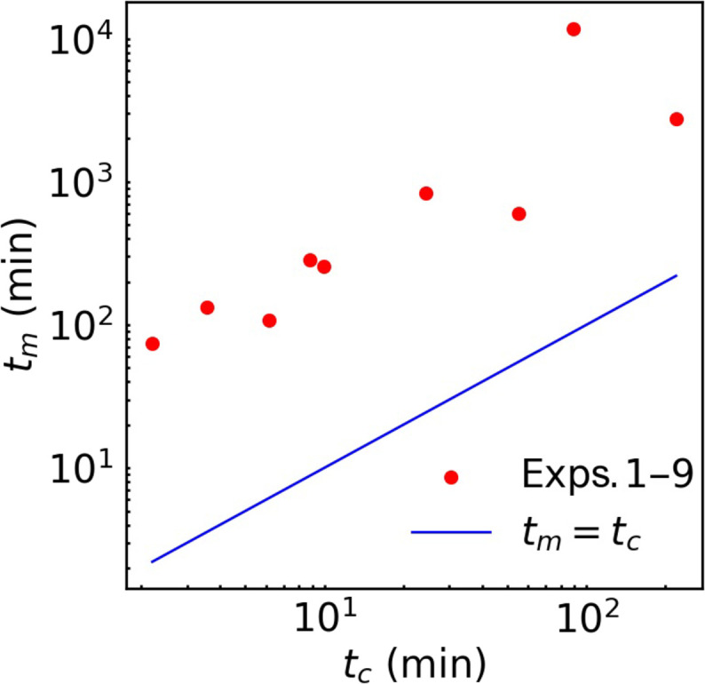
Experimental melting time t_m for all experiments are recorded and plotted against the characteristic convective relaxation time t_c. We found that t_m >> t_c. The blue line represents the reference line of t_m = t_c.

Therefore, we propose a pseudo-steady-state hypothesis: The flow field of the melted zone develops to a steady state (or completely developed state with time-averaged features unchanged) before the melting front moves. Thus, we do not need to consider the dynamics of the initialization and development of R-D convection (54) for the demonstrative numerical simulation and can focus only on the “ultimate regime” (28, 33), with a constant density contrast.

Wavelength analysis

Raw data

The melting front morphology was captured by image processing. We analyzed the front using FFT and obtained the frequency-amplitude correlation. Amplitude is made dimensionless by normalization with the cell length, L. For each frequency $f_i$ with amplitude $e_{i,\mathit{raw}}$, the corresponding wavelength is calculated as ${\mathrm{\lambda }}_i=1/f_i$. For wavelength ${\mathrm{\lambda }}_i$, the corresponding “wave energy” is defined as $f_i{e}_{i,\mathit{raw}}^2$, which is an analog from signal processing technologies. We eliminate data for ${\mathrm{\lambda }}_i\ge L$.

Denoising

The discretization of the front morphology into pixels results in long-tail noise at the high-frequency end, which falsifies the wavelength analysis. To quantify the noise, we analyze the high-frequency information ($n_i$ > 200) and indicate that $f_i{e}_{i,\mathit{raw}}^2$ at high frequency randomly fluctuates around an average P value, with an SD of $\mathrm{\delta }E$. We subsequently obtain denoised $e_i$ by solving Eq. 3; the details are shown in figs. S3 and S7 in the Supplementary Materials

$$f_i{e}_i^2=\{\begin{array}{cc}0,\hfill & \text{if} P+\mathrm{\delta }E\ge f_i{e}_{i,\mathit{raw}}^2\hfill \\ f_i{e}_{i,\mathit{raw}}^2-P,\hfill & \text{if} P+\mathrm{\delta }E<f_i{e}_{i,\mathit{raw}}^2\hfill \end{array}$$ (3)

Average wavelength and maximum amplitude

The average wavelength λ is calculated by $\mathrm{\lambda }=\frac{\sum e_i^2}{\sum f_i{e}_i^2}$. We defined the maximum among all $e_i$ values as $e_{\mathit{max}}$ to represent the magnitude of the front instability.

Supplementary Materials

The PDF file includes:

Supplementary Text

Figs. S1 to S3

Legends for movies S1 to S11

Other Supplementary Material for this manuscript includes the following:

Movies S1 to S11

REFERENCES AND NOTES

- 1.Guimond J. A., Mohammed A. A., Walvoord M. A., Bense V. F., Kurylyk B. L., Saltwater intrusion intensifies coastal permafrost thaw. Geophys. Res. Lett. 48, e2021GL094776 (2021). [Google Scholar]
- 2.Anthony K. M. W., Zimov S. A., Grosse G., Jones M. C., Anthony P. M., Chapin F. S., Finlay J. C., Mack M. C., Davydov S., Frenzel P., Frolking S., A shift of thermokarst lakes from carbon sources to sinks during the Holocene epoch. Nature 511, 452–456 (2014). [DOI] [PubMed] [Google Scholar]
- 3.Olson S., Jansen M. F., Abbot D. S., Halevy I., Goldblatt C., The effect of ocean salinity on climate and its implications for earth’s habitability. Geophys. Res. Lett. 49, e2021GL095748 (2022). [DOI] [PMC free article] [PubMed] [Google Scholar]
- 4.Schuur E. A. G., McGuire A. D., Schädel C., Grosse G., Harden J. W., Hayes D. J., Hugelius G., Koven C. D., Kuhry P., Lawrence D. M., Natali S. M., Olefeldt D., Romanovsky V. E., Schaefer K., Turetsky M. R., Treat C. C., Vonk J. E., Climate change and the permafrost carbon feedback. Nature 520, 171–179 (2015). [DOI] [PubMed] [Google Scholar]
- 5.Whiteman G., Hope C., Wadhams P., Vast costs of Arctic change. Nature 499, 401–403 (2013). [DOI] [PubMed] [Google Scholar]
- 6.Schuur E. A. G., Bockheim J., Canadell J. G., Euskirchen E., Field C. B., Goryachkin S. V., Hagemann S., Kuhry P., Lafleur P. M., Lee H., Mazhitova G., Nelson F. E., Rinke A., Romanovsky V. E., Shiklomanov N., Tarnocai C., Venevsky S., Vogel J. G., Zimov S. A., Vulnerability of permafrost carbon to climate change: Implications for the global carbon cycle. Bioscience 58, 701–714 (2008). [Google Scholar]
- 7.Mishra U., Hugelius G., Shelef E., Yang Y., Strauss J., Lupachev A., Harden J. W., Jastrow J. D., Ping C.-L., Riley W. J., Schuur E. A. G., Matamala R., Siewert M., Nave L. E., Koven C. D., Fuchs M., Palmtag J., Kuhry P., Treat C. C., Zubrzycki S., Hoffman F. M., Elberling B., Camill P., Veremeeva A., Orr A., Spatial heterogeneity and environmental predictors of permafrost region soil organic carbon stocks. Sci. Adv. 7, eaaz5236 (2021). [DOI] [PMC free article] [PubMed] [Google Scholar]
- 8.Wang T., Yang D., Yang Y., Piao S., Li X., Cheng G., Fu B., Permafrost thawing puts the frozen carbon at risk over the Tibetan Plateau. Sci. Adv. 6, eaaz3513 (2020). [DOI] [PMC free article] [PubMed] [Google Scholar]
- 9.Mohammed A. A., Bense V. F., Kurylyk B. L., Jamieson R. C., Johnston L. H., Jackson A. J., Modeling reactive solute transport in permafrost-affected groundwater systems. Water Resour. Res. 57, e2020WR028771 (2021). [Google Scholar]
- 10.R. Margesin, Ed., Permafrost Soils, vol. 16 of Soil Biology (Springer Berlin Heidelberg, 2009). [Google Scholar]
- 11.Burkow I. C., Kallenborn R., Sources and transport of persistent pollutants to the Arctic. Toxicol. Lett. 112–113, 87–92 (2000). [DOI] [PubMed] [Google Scholar]
- 12.Dyke L. D., Contaminant migration through the permafrost active layer, Mackenzie Delta area, Northwest Territories, Canada. Polar Rec. 37, 215–228 (2001). [Google Scholar]
- 13.De Bruin J. G. H., Bense V. F., Van Der Ploeg M. J., Inferring permafrost active layer thermal properties from numerical model optimization. Geophys. Res. Lett. 48, e2021GL093306 (2021). [Google Scholar]
- 14.Feltham D. L., Untersteiner N., Wettlaufer J. S., Worster M. G., Sea ice is a mushy layer. Geophys. Res. Lett. 33, L14501 (2006). [Google Scholar]
- 15.Notz D., Worster M. G., Desalination processes of sea ice revisited. J. Geophys. Res. 114, C05006 (2009). [Google Scholar]
- 16.Feltham D. L., Grae Worster M. G., Flow-induced morphological instability of a mushy layer. J. Fluid Mech. 391, 337–357 (1999). [Google Scholar]
- 17.Worster M. G., Wettlaufer J. S., Natural convection, solute trapping, and channel formation during solidification of saltwater. J. Phys. Chem. B 101, 6132–6136 (1997). [Google Scholar]
- 18.Worster M. G., Natural convection in a mushy layer. J. Fluid Mech. 224, 335–359 (1991). [Google Scholar]
- 19.Guo R., Sun H., Zhao Q., Li Z., Liu Y., Chen C., A novel experimental study on density-driven instability and convective dissolution in porous media. Geophys. Res. Lett. 48, e2021GL095619 (2021). [Google Scholar]
- 20.Du Y., Wang Z., Jiang L., Calzavarini E., Sun C., Sea water freezing modes in a natural convection system. J. Fluid Mech. 960, A35 (2023). [Google Scholar]
- 21.Cohen C., Berhanu M., Derr J., Du Pont S. C., Buoyancy-driven dissolution of inclined blocks: Erosion rate and pattern formation. Phys. Rev. Fluids 5, 053802 (2020). [Google Scholar]
- 22.Favier B., Purseed J., Duchemin L., Rayleigh–Bénard convection with a melting boundary. J. Fluid Mech. 858, 437–473 (2019). [Google Scholar]
- 23.Mondal M., Gayen B., Griffiths R. W., Kerr R. C., Ablation of sloping ice faces into polar seawater. J. Fluid Mech. 863, 545–571 (2019). [Google Scholar]
- 24.Rayleigh L., LIX. On convection currents in a horizontal layer of fluid, when the higher temperature is on the under side. Lond. Edinb. Dublin Philos. Mag. J. Sci. 32, 529–546 (1916). [Google Scholar]
- 25.Schubert G., Straus J. M., Three-dimensional and multicellular steady and unsteady convection in fluid-saturated porous media at high Rayleigh numbers. J. Fluid Mech. 94, 25–38 (1979). [Google Scholar]
- 26.Horton C. W., Rogers F. T., Convection currents in a porous medium. J. Appl. Phys. 16, 367–370 (1945). [Google Scholar]
- 27.De Paoli M., Pirozzoli S., Zonta F., Soldati A., Strong Rayleigh–Darcy convection regime in three-dimensional porous media. J. Fluid Mech. 943, A51 (2022). [Google Scholar]
- 28.Hewitt D. R., Neufeld J. A., Lister J. R., Ultimate regime of high Rayleigh number convection in a porous medium. Phys. Rev. Lett. 108, 224503 (2012). [DOI] [PubMed] [Google Scholar]
- 29.Paoli M., Convective mixing in porous media: A review of Darcy, pore-scale and Hele-Shaw studies. Eur. Phys. J. E Soft Matter 46, 129 (2023). [DOI] [PMC free article] [PubMed] [Google Scholar]
- 30.Lapwood E. R., Convection of a fluid in a porous medium. Math. Proc. Camb. Philos. Soc. 44, 508–521 (1948). [Google Scholar]
- 31.Molz F., Advection, dispersion, and confusion. Groundwater 53, 348–353 (2015). [DOI] [PubMed] [Google Scholar]
- 32.Liang Y., Wen B., Hesse M. A., DiCarlo D., Effect of dispersion on solutal convection in porous media. Geophys. Res. Lett. 45, 9690–9698 (2018). [Google Scholar]
- 33.Pirozzoli S., De Paoli M., Zonta F., Soldati A., Towards the ultimate regime in Rayleigh–Darcy convection. J. Fluid Mech. 911, R4 (2021). [Google Scholar]
- 34.Wen B., Corson L. T., Chini G. P., Structure and stability of steady porous medium convection at large Rayleigh number. J. Fluid Mech. 772, 197–224 (2015). [Google Scholar]
- 35.De Paoli M., Zonta F., Soldati A., Influence of anisotropic permeability on convection in porous media: Implications for geological CO2 sequestration. Phys. Fluids 28, 056601 (2016). [Google Scholar]
- 36.Lasser J., Nield J. M., Ernst M., Karius V., Wiggs G. F. S., Threadgold M. R., Beaume C., Goehring L., Salt polygons and porous media convection. Phys. Rev. X. 13, 011025 (2023). [Google Scholar]
- 37.Lagziri H., Bezzazi M., Robin boundary effects in the Darcy–Rayleigh problem with local thermal non-equilibrium model. Transp. Porous Media 129, 701–720 (2019). [Google Scholar]
- 38.Caldwell D. R., Thermal and Fickian diffusion of sodium chloride in a solution of oceanic concentration. Deep-Sea Res. Oceanogr. Abstr. 20, 1029–1039 (1973). [Google Scholar]
- 39.Vancoppenolle M., Goosse H., de Montety A., Fichefet T., Tremblay B., Tison J. L., Modeling brine and nutrient dynamics in Antarctic sea ice: The case of dissolved silica. J. Geophys. Res. 115, C02005 (2010). [Google Scholar]
- 40.Carman P. C., Permeability of saturated sands, soils and clays. J. Agric. Sci. 29, 262–273 (1939). [Google Scholar]
- 41.Magnani M., Musacchio S., Provenzale A., Boffetta G., Convection in the active layer speeds up permafrost thaw in coarse-grained soils. Phys. Rev. Fluids 9, L081501 (2024). [Google Scholar]
- 42.Zhu X., Fu Y., De Paoli M., Transport scaling in porous media convection. J. Fluid Mech. 991, A4 (2024). [Google Scholar]
- 43.S. V. Patankar, Numerical Heat Transfer and Fluid Flow, Series in Computational Methods in Mechanics and Thermal Sciences (McGraw-Hill, 1980) [u.a.]. [Google Scholar]
- 44.Bijeljic B., Blunt M. J., Pore-scale modeling of transverse dispersion in porous media. Water Resour. Res. 43, W12S11 (2007). [Google Scholar]
- 45.Menand T., Woods A. W., Dispersion, scale, and time dependence of mixing zones under gravitationally stable and unstable displacements in porous media. Water Resour. Res. 41, W05014 (2005). [Google Scholar]
- 46.Pickens J. F., Grisak G. E., Modeling of scale-dependent dispersion in hydrogeologic systems. Water Resour. Res. 17, 1701–1711 (1981). [Google Scholar]
- 47.Pang L., Hunt B., Solutions and verification of a scale-dependent dispersion model. J. Contam. Hydrol. 53, 21–39 (2001). [DOI] [PubMed] [Google Scholar]
- 48.E. J. Peters, Advanced Petrophysics: Geology, Porosity, Absolute Permeability, Heterogeneity, and Geostatistics (Live Oak Book Company, 2012). [Google Scholar]
- 49.Arya A., Hewett T. A., Larson R. G., Lake L. W., Dispersion and reservoir heterogeneity. SPE Reserv. Eng. 3, 139–148 (1988). [Google Scholar]
- 50.Saffman P., Taylor G., The penetration of a fluid into a porous medium or Hele-Shaw cell containing a more viscous liquid. Proc. R. Soc. London Ser. A Math. Phys. Sci. 245, 312–329 (1958). [Google Scholar]
- 51.DiCarlo D. A., Stability of gravity-driven multiphase flow in porous media: 40 years of advancements. Water Resour. Res. 49, 4531–4544 (2013). [Google Scholar]
- 52.Schwerdtfecer P., The thermal properties of sea ice. J. Glaciol. 4, 789–807 (1963). [Google Scholar]
- 53.R. B. Bird, W. E. Stewart, E. N. Lightfoot, Transport Phenomena (John Wiley & Sons, rev. ed. 2, 2006). [Google Scholar]
- 54.De Paoli M., Perissutti D., Marchioli C., Soldati A., Experimental assessment of mixing layer scaling laws in Rayleigh-Taylor instability. Phys. Rev. Fluids 7, 093503 (2022). [Google Scholar]
Associated Data
This section collects any data citations, data availability statements, or supplementary materials included in this article.