Hybrid Gaussian process regression with temporal feature extraction for partially interpretable remaining useful life interval prediction in Aeroengine prognostics

Abstract

The estimation of Remaining Useful Life (RUL) plays a pivotal role in intelligent manufacturing systems and Industry 4.0 technologies. While recent advancements have improved RUL prediction, many models still face interpretability and compelling uncertainty modeling challenges. This paper introduces an adapted Gaussian Process Regression (GPR) model for RUL interval prediction, tailored for the complexities of manufacturing process development. The adapted GPR predicts confidence intervals by learning from historical data and addresses uncertainty modeling in a more structured way. The approach effectively captures intricate time-series patterns and dynamic behaviors inherent in modern manufacturing systems by coupling GPR with deep adaptive learning-enhanced AI process models. Moreover, the model evaluates feature significance to ensure more transparent decision-making, which is crucial for optimizing manufacturing processes. This comprehensive approach supports more accurate RUL predictions and provides transparent, interpretable insights into uncertainty, contributing to robust process development and management.

Introduction

Prognostics and Health Management (PHM) plays a crucial role in increasing equipment availability, reducing maintenance costs, and improving the scheduling of maintenance events. By predicting potential failures, maintenance activities can be planned, reducing downtime and allowing for more efficient operations in manufacturing environments¹. Predicting a machine’s Remaining Useful Life (RUL) using real-time condition data is central to effective prognostics². With modern machines continuously collecting sensor data at frequent intervals, this data forms a time series with inherent temporal characteristics. Consequently, RUL prediction involves solving a time series regression problem that captures both the operational and mechanical characteristics of the machinery³.

Like many other time series prediction challenges, RUL estimation methods can be divided into two main categories: learning-based and model-based approaches. Learning-based methods utilize machine learning and deep learning techniques, such as long short-term memory⁴and transformer⁵, which leverage historical data to improve predictions. These methods rely on supervised learning to achieve accurate outcomes. In manufacturing processes, it is critical to incorporate temporal continuity and system behavior dynamics when dealing with high-dimensional data. However, many traditional machine learning methods focus solely on single-point predictions without quantifying uncertainty.

Model-based approaches, on the other hand, include both physical and statistical methods. Physical approaches involve building models that represent the underlying mechanical systems. Implementing this approach necessitates intricate physical modeling, thereby constraining its feasibility for broader, real-world applications⁶. In contrast, statistical methods, particularly Gaussian Process Regression (GPR), which provides accurate predictions even with small datasets, as well as interpretability of the sources of uncertainty, offer a more flexible way of predicting RUL^7,8. GPR is a non-parametric Bayesian approach that effectively models diverse deterioration mechanisms and outputs uncertainty measures, making it highly applicable in complex systems where physical models may fail^9,10. Despite its robustness in generating prediction intervals, GPR alone may face challenges in handling large-scale time-series data typical of industrial environments. Specifically, GPR involves calculating and storing an covariance matrix (where n is the number of data points), resulting in a computational complexity of and a memory complexity of .

This paper proposes a novel Hybrid Gaussian process Regression with temporal feature extraction for partially interpretable RUL interval Prediction in aero-engine prognostics (HRP) to overcome the limitations of both learning and model-based approaches. The approach leverages an adapted GPR model, pre-trained on time-series data, to incorporate temporal dynamics and system behaviors relevant to intelligent manufacturing systems. Unlike single learning-based methods, this method captures uncertainty and key predictive features without relying solely on black-box neural networks by modifying GPR into deep adaptive learning-enhanced regression. The pre-processing steps ensure that the adapted GPR adaptively utilizes feature representation and system diagnostics to increase robustness compared to single model-based methods. Additionally, the model identifies and prioritizes critical physical features contributing to system degradation, enhancing predictive accuracy and enabling optimal maintenance decisions. Our model is validated using the NASA urbofan engine dataset (CMAPSS) and we conducted experiments on wafer test machines in the semiconductor industry. The RUL is typically measured in years and is quantified by identifying the point of failure.

The key contributions of this paper are as follows:

• A supervised GPR model with temporal feature extraction is proposed to reflect system health states in manufacturing environments. This model is specifically tailored to capture the time-dependent degradation of machinery, enhancing predictive insights into system performance over time.

• Confidence intervals generated by the GPR model quantify the uncertainty of predicted RUL, offering a dual advantage: improved prediction accuracy and a more precise assessment of failure risk.

• Feature importance analysis is incorporated to identify key contributors from mechanical and sensor data, providing actionable insights into degradation factors. The model facilitates real-time, data-driven maintenance planning by integrating uncertainty modeling and adaptive learning techniques.

The rest of this paper is organized as follows: First, we introduce the preliminaries and outline the proposed method. Then, we discuss the experimental results and analysis. Finally, we summarize the findings and discuss future directions for RUL estimation in smart manufacturing environments.

Related works

RUL prediction has been a critical area of research in prognostics and health management for enhancing equipment availability and reducing downtime. While various methods have been proposed, most approaches face challenges in balancing predictive accuracy with interpretability and uncertainty quantification. Historically, learning-based methods, such as long short-term memory networks and Transformer models, have been widely used for RUL prediction due to their ability to capture temporal dynamics in sequential data^11,12. Liu et al¹³. integrated clustering analysis with LSTM to enhance prediction accuracy. In contrast, Wang et al¹⁴. combined adaptive sliding windows with LSTM to predict the performance of lithium-ion batteries. However, these methods focus on point predictions and often lack interpretability, especially regarding feature significance and uncertainty quantification. Additionally, while LSTM models effectively capture sequential patterns, they frequently function as black-box models, providing little insight into the underlying mechanics of degradation processes.

Researchers employ statistical methods like GPR for RUL prediction to address these limitations, offering a more interpretable and flexible approach. GPR, as a non-parametric Bayesian technique, provides both point estimates and confidence intervals, thus quantifying uncertainty in predictions^9,10. This makes GPR particularly valuable in scenarios where the complexity of machinery precludes purely physical modeling⁶. For example, Hong et al¹⁵. applied GPR to predict bearing RUL by modeling the relationship between time-domain features and future operational states. Similarly, Baraldi et al¹⁶. demonstrated the utility of GPR in modeling creep growth in materials, providing reliable prediction intervals for degradation processes.

However, despite its advantages in uncertainty quantification, GPR faces challenges in processing large-scale time-series data, which is typical in industrial applications. Previous studies have shown that GPR’s scalability can be a limitation when handling high-dimensional datasets. Some researchers have explored hybrid approaches that integrate GPR with other learning techniques to mitigate this. For instance, Pang et al¹⁷. employed fuzzy information granulation with least squares support vector machines to enhance time interval forecasting for lithium-ion batteries. However, such methods still rely heavily on feature engineering and lack adaptive learning capabilities.

Our method enhances GPR by incorporating temporal dynamics through adaptive learning, enabling it to handle large datasets and improve uncertainty modeling. This approach bridges interpretability, uncertainty quantification, and predictive accuracy for RUL estimation, making it well-suited for Industry 4.0 applications. In summary, this work combines machine learning and statistical modeling to provide a transparent, robust solution for real-time, data-driven maintenance in industrial settings.

Methods

This section begins by formulating the multi-dimensional time series problem in RUL prediction. Then, an overview of our interval prediction framework is provided. The model is referred to using the acronym HRP. After that, we introduce the details of the model’s main elements.

Problem definition

Given run-to-failure data for several mechanical systems, denoted as and corresponding RUL: , where 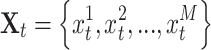represents observations at the corresponding running time t and M represents the number of monitoring sensors. If Life represents the total operational life of a machine, the RUL of time t is calculated by . The objective is to find a mapping from high-dimensional observations to a scalar value, defined as . Given new data , estimates of can be obtained as , and the confidence interval is predicted, where and represent estimated lower and upper bounds of respectively. Simultaneously, the influence of the M monitoring sensors on faults is analyzed, enabling the estimation of sensor impact factors .

Framework overview

The dual-line interval RUL prediction strategy, illustrated in Fig.1, consists of two key stages: offline training and online prediction. This strategy provides engineers with two crucial outputs: the sensor influence on fault modes and the predicted interval for the RUL. Initially, all data follow the same preprocessing pipeline, including sensor selection, normalization, smoothing, and sliding window process. During training, our model is trained with data from known run-to-failure cycles, aligning the real RUL with a health index. The trained model serves both as a callable real-time prediction tool and a mechanism to provide insights into the relative importance of features during fault cycles. In the test phase, incomplete degradation trajectories from the test data are processed in real time, providing rapid predictions of the remaining degradation trajectories using the trained network.

Fig. 1.

Dual-line interval RUL prediction framework.

The detailed structure of our model is depicted in Fig. 2, and follows a series of steps. Firstly, after data have been preprocessed, raw data are converted into the format , which serves as the input to the network. Secondly, temporal feature extraction adopts mathematical techniques for managing temporal information flow. Adaptive filtering and time-series compression gated memory cells preserve long-term dependencies, ensuring that relevant historical data are retained in the feature set while discarding noise or less significant information. This preprocessing step compresses the sequence of high-dimensional sensor data into a lower-dimensional latent space with a dimension of . The extracted time-series features are then fed to train mean function and the covariance function in multivariate normal Gaussian distribution, which not only learns the distribution of the data but also generates prediction intervals for RUL with quantified uncertainty. The model’s ability to capture temporal dynamics and probabilistically represent the system’s health status is crucial for accurately predicting the RUL and quantifying the associated uncertainty, which significantly enhances its performance. Furthermore, our model performs feature importance analysis based on how different sensors contribute to the fault modes, providing engineers with a clearer understanding of the degradation process. In the final step, engineers can conduct a comprehensive run-to-failure assessment based on the prediction intervals produced by adapted GPR and the detailed feature analysis. This process allows for both predictive insights and interpretability, combining the power of advanced temporal modeling with the flexibility and uncertainty quantification of adapted GPR.

Fig. 2.

Illustration of the network in our method HRP.

Data preprocessing

We employ a four-step procedure to process the original dataset to ensure the data is prepared for practical prognostics analysis. First, we perform feature selection. After an extensive review of the sensor signals, 14 critical sensors are retained, providing the most significant information for accurate RUL predictions. Additionally, we utilize a piecewise linear degradation model to model the RUL as described in previous research¹⁸. Here, the time for the change point is set at 125. Second, we apply z-score normalization to the sensor signals for each instance, standardizing the readings to improve model performance and comparability across different sensors¹⁹. This normalization transforms the original time series , corresponding to the j-th sensor of the i-th sample, as formula , where and represent the mean value and the standard deviation deviation, respectively, for the j-th sensor readings across all instances in each dataset. Third, we implement exponential smoothing¹⁸to retain the underlying trends in sensor signals while minimizing the impact of noise and short-term fluctuations. This technique improves the accuracy of predictive models by focusing on long-term degradation trends. Finally, we segment the preprocessed data using a sliding window approach²⁰. This method partitions the entire time series into smaller, equal-length windows. The window length is determined based on prior empirical studies²¹, ensuring it captures sufficient temporal information for reliable prediction. Detailed descriptions of these four preprocessing steps, including parameters and justifications, are provided in the Supplementary Materials S2.

Temporal feature extraction

Advanced temporal feature extraction methods are employed during pre-analysis to enhance the model’s ability to capture temporal dependencies. These methods are based on the mathematical principles of sequential learning, which allow the model to retain and process long-term and short-term dependencies inherent in time-series data. The method utilizes gating mechanisms that control the flow of information through the model, mimicking how LSTM networks handle temporal data through input control, memory retention, and output management^4,22. Detailed mathematical expressions are provided in the Supplementary Materials S3. Once the temporal features from input have been extracted, they are formatted into hidden states , which encapsulate the most important information from the time-series. These hidden states, which compress the multivariate time series into a reduced form, are then transferred to the next processing stage, adapted GPR, where distribution learning occurs, and feature importance analysis is performed. The hidden states can be expressed as

1

Here, represents the learnable parameters of the feature extraction process and m stands for the hidden layer size.

The loss function used to optimize the feature extraction process is designed to handle outliers in the data by employing a Huber loss, which combines the benefits of squared error and absolute error, defined as:

2

In this way, the extracted features retain the sequence’s temporal dynamics while ensuring stability in the training process. They are also tailored to the requirements of the Gaussian Process framework for further learning.

Adapted GPR

We modify GPR cooperated with temporal learning to adaptively describe uncertainty. Adapted GPR receives the hidden state as defined by equation (1), and estimates outputs and confidence interval . A Gaussian process (GP) is a collection of random variables, where any finite subset that adheres to a joint Gaussian distribution. For any input , the probability distribution of the corresponding RUL follows a multivariate normal Gaussian distribution. The GP is characterized by two essential components, the mean function and the covariance function , which jointly specify its probability distribution,

3

Generally, the mean function is selected as a zero-mean function, and the covariance function is the squared exponential function, defined as

4

where represents the characteristic length-scale, and represents the amplitude of the covariance. Therefore, the mean vector is given by , and the n-by-n covariance matrix is given by 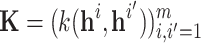. Our method HRP assumes that the observations are noisy realizations of the GP prior. The noise is typically modeled as a Gaussian distribution with zero mean and variance . Given these assumptions, the prior distribution follows a multivariate normal distribution, where denotes the m-by-m identity matrix,

5

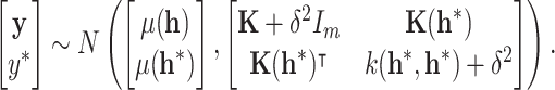
The core strength of GPR lies in its ability to infer a posterior distribution over functions that map the sensor readings to the RUL based on the observed data . This distribution provides a point estimate at any given time t and a measure of uncertainty as a confidence interval. This predictive distribution is central to prognostics as it naturally quantifies the uncertainty of the RUL prediction. In the application stage of prediction, when a new sampled from historical data is observed, temporal learning processes it into . The joint prior Gaussian distribution of the training RUL and is obtained as follows,

6

The posterior mean function and covariance functions are given by

7

8

where , the mean of RUL can be predicted using , assuming a prior. The prediction is obtained as

9

It is important to acknowledge that no prediction can be completely accurate, and prediction errors cannot be eliminated. To address this issue, we propose a straightforward approach providing a prediction interval such that

10

where 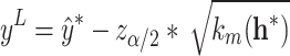, , and represents the quantile of the corresponding standard normal distribution.Generally, when , the lower bound is and the upper bound is . This predictive distribution is central to prognostics as it naturally quantifies the uncertainty of the RUL prediction.

In summary, GPR offers a probabilistic framework for RUL prediction that effectively accommodates the temporal dynamics inherent in prognostic processes. Additionally, it systematically quantifies uncertainty. The flexibility of adapted GPR to analyze contributions from individual sensors further enhances its applicability for fault diagnosis and prognostics in complex mechanical systems.

Importance analysis

A feature importance analysis is integrated into the model to determine which sensors most significantly influence the RUL. This analysis is based on evaluating the impact of each feature, derived from sensor data, on the RUL predictions. The feature importance assessment begins by inputting the hidden state , defined by equation (1), into the analysis component. This hidden state encapsulates the relevant temporal features extracted during the data preprocessing and temporal feature extraction stages. The output of this process is a set of feature importance scores , where each corresponds to a sensor feature, and a higher value indicates a more significant contribution to the machine’s degradation and, thus, the RUL prediction.

The model evaluates feature importance by systematically altering the input features and measuring the corresponding changes in prediction accuracy. Specifically, it compares the accuracy of the full model against a version where each feature is individually permuted. Permutation involves randomly shuffling a given feature’s values while keeping the others intact, disrupting its relationship with the output. By observing the decline in accuracy after this permutation, the model quantifies the importance of that specific feature. If the prediction accuracy significantly decreases, it implies that the feature in question plays a critical role in predicting RUL. Conversely, the feature is deemed less necessary if there is little to change.

This approach allows for an interpretability layer in the model, making it possible to identify which sensors are most likely to influence the degradation process. By ranking the features based on their importance scores, engineers can gain insights into which sensor data are the primary contributors to the machine’s health decline and may indicate fault-prone areas in the system. This information is invaluable for maintenance planning, as it allows engineers to focus on the most critical sensor readings and take preventative actions based on the insights from the feature importance analysis.

The methodology of feature evaluation is inspired by the way decision trees assess the relevance of each input feature in complex models^23,24. The ranking produced by this process directly supports more effective and interpretable predictions in the context of fault diagnosis and predictive maintenance.

Experimental setup

Dataset description

We show the efficacy of the suggested approach using the C-MAPSS dataset as a benchmark. ’Commercial Modular Aero-Propulsion System Simulation’, or C-MAPSS, is a NASA tool that simulates extensive commercial turbofan engine data using Matlab Simulink. C-MAPSS dataset is created using the C-MAPSS simulator²⁵. Four subsets exist, from FD001 to FD004, within the dataset¹⁸. Twenty-one sensor measurements are gathered at each observation time, providing comprehensive information on engine locations and operational conditions. In the training set, each engine initially operates normally but starts to deteriorate after a specific time. Conversely, the test set comprises incomplete data, with time series terminating before the onset of engine degradation²⁶. The aim is to estimate each engine’s remaining operable cycle count. The complete introduction of the dataset can be found in Supplementary Material S1.

Configuration setting

The architecture is implemented using Python 3.7 and the PyTorch 1.13.1 (GPU version) framework. The hardware configuration includes an Intel(R) Xeon(R) Platinum 8380 CPU, eight RTX 3090 GPUs, and 500 GB of RAM. Detailed descriptions of the network setting, including architecture and parameters, are provided in the Supplementary Materials S5.

Evaluation setting

To evaluate the model’s performance, we utilize three functions. The first is the root mean square error (RMSE)²⁷. Define , representing the difference between the predicted and true RUL values. RMSE is calculated using

11

where M denotes the number of engines. The lower the RMSE score, the more accurate the interval prediction.

Two additional functions, average coverage interval length and coverage probability, are utilized to assess the model’s interval prediction performance. Normalized averaged width (NAW) measures the average width of the constructed predicted intervals as a percentage of the underlying target range. The definition of NAW is provided as follows,

12

where R represents the range of the target variable throughout the forecast period. Predicted intervals with lower NAW values are considered more effective.

The coverage width-based criterion (CWC) provides a comprehensive evaluation score based on coverage probability and NAW. The fundamental concept behind CWC is that the score should be high irrespective of interval width if coverage probability is below the nominal confidence level. At the same time, NAW becomes the dominant factor if coverage probability exceeds this level. The definition of CWC is

13

where , where if , and otherwise. A lower CWC score indicates a more effective interval prediction.

Results

Feature learning analysis

Figure 3 displays the kernel density estimates (KDE) for sub-dataset FD001, providing the probability density function (PDF) of the 14 features individually. Besides, we provide importance ranking underneath. Since the other three sub-datasets exhibit similar trends and patterns, the Supplementary Materials S4 give the full results.

Fig. 3.

Distribution and importance for sub-dataset FD001. Red dashed lines represent the density of testing datasets, and blue lines represent the density of training datasets. The lower figure shows the importance ranking of 14 features. It indicates that feature 6, which corresponds to the physical core speed, exerts the greatest influence.

KDE provides a non-parametric approach to estimating a random variable’s PDF. The default Gaussian kernel is used. The coincident density curves demonstrate strong consistency in the PDFs across the test and training datasets, thereby validating the use of GPR on the dataset. The histogram of importance shows that Feature 6 is the most important in FD001, demonstrating its robustness and significant predictive power across these datasets. Engineers can optimize the engine by focusing on the most influential variables, such as Features 6, 10, and 13.

Prognostic results analysis

To further test the performance of our model, eight engines, two from each of the four test datasets, are randomly selected. The actual RUL curves and online RUL interval estimation results for the test set, at a 95% confidence level, are presented in Fig. 4. The errors between ground truth and predicted points are plotted in Fig. 4. The lower segment shows that although the predicted RUL does not always match the actual RUL, it does not lead to poor judgment. The predicted intervals, composed of upper and lower prediction limits, appropriately cover the target values. As service time progresses, the upper and lower prediction limits closely follow the actual value changes. Although the predicted RUL sometimes exceeds the actual RUL, the predicted intervals consistently cover the real RUL, demonstrating the utility of the proposed method for constructing prediction intervals to capture fault trends.

Fig. 4.

RUL prognostic performances of our algorithm for the testing engine units in four sub-datasets. The blue polyline represents the actual RUL. The range between the red curve and the green curve represents the predicted interval. The red segment indicates that the predicted RUL exceeds the actual RUL, misleading engineers into believing the machine can still operate. Conversely, the green segment signifies that the predicted RUL is less than the actual RUL. Engine 46 and 62 belong to FD001. Engine 145 and 185 belong to FD002. Engine 20 and 99 belong to FD003. Engine 32 and 68 belong to FD004.

Comparison with the state-of-the-art methods

To provide a comprehensive evaluation of each model’s performance under various operating conditions and to facilitate a clear comparison of their strengths and limitations, the key metrics RMSE (11), NAW (12), and CWC (13) have been calculated for each algorithm. As shown in Table 1, our proposed method achieves commendable RMSE results across the four sub-datasets, outperforming most established methods in most cases. This highlights the robustness of our approach in accurately predicting RUL, especially under complex conditions. The results are particularly noteworthy for the FD002 subset, encompassing more challenging operational settings with diverse fault modes. While the performance of our model on sub-datasets FD001 and FD003 does not achieve the absolute best RMSE, it remains competitive and within the lower range of error rates compared to other models. This indicates that even in cases where our model does not achieve the top score, it still provides a highly reliable prediction with minimal deviation, ensuring robust and consistent results across varying conditions. This consistency is essential for practical applications in industrial prognostics, as it supports dependable predictions regardless of the specific operational scenario.

Table 1.

Comparison of different models on RMSE.

Models	FD001	FD002	FD003	FD004
D-LSTM28, 2017	16.14	24.49	16.18	28.17
BS-LSTM29, 2018	14.89	26.86	15.11	27.11
BL-CNN30, 2019	13.18	19.09	13.75	20.97
RF-LSTM31, 2020	16.87	23.91	17.89	25.49
CNN-LSTM32, 2021	11.56	17.67	12.98	20.19
DA-Transformer21, 2022	12.25	17.08	13.39	19.86
IDMFFN33, 2023	12.18	19.17	11.89	21.72
HRP(Ours)	13.09	12.33	13.49	19.65

In addition to the RMSE analysis, an interval comparison for the parameters NAW and CWC is provided in Table 2. These metrics offer insights into the reliability and precision of the prediction intervals produced by each model. Across all four sub-datasets, our approach consistently reduces NAW values by at least 50.70% on average compared to other models. This reduction demonstrates the model’s capability to provide tighter prediction intervals, which are desirable for practical applications where narrow intervals indicate higher confidence in the predictions. Furthermore, the CWC values, which combine interval width and coverage probability to evaluate the overall quality of prediction intervals, also significantly improve. On the first three sub-datasets, FD001, FD002, and FD003, our method achieves an average CWC reduction of at least 50.16%, suggesting that the intervals become narrower and maintain appropriate coverage. This balance of narrow intervals with adequate coverage reflects high accuracy and reliability, essential for predicting RUL in smart manufacturing settings. Out of the four sub-datasets, our method consistently outperforms existing approaches, providing the most reliable and interpretable intervals. This suggests that our model holds considerable promise for effectively predicting faults in advance, contributing to robust maintenance planning and improved operational safety in industrial systems. Ablation study about kernel setting in GPR is provided in the Supplementary Materials S6.

Table 2.

Comparison of different models on interval criterions.

Models	FD001		FD002		FD003		FD004
	NAW(%)	CWC(%)	NAW(%)	CWC(%)	NAW(%)	CWC(%)	NAW(%)	CWC(%)
LSTMBS29,2018	37.70	83.90	47.20	89.20	45.90	102.15	65.40	170.80
IESGP34, 2019	54.00	59.68	55.70	137.00	44.50	93.27	49.10	248.11
AGCNN35, 2023	48.06	97.00	59.29	98.46	44.26	97.00	63.48	95.56
HRP(Ours)	21.00	38.48	29.00	s76.06	23.00	27.94	28.00	468.43

Conclusion

This paper proposes an intelligent RUL interval prediction method based on a adapted GPR network for aero-engines. We embedded a temporal feature extraction into regression, enhancing the accuracy and robustness of RUL interval predictions. As an effective regression method, GPR is modified to adapt to engineering properties in our network, which comprehensively learns the diversity of distributions between sensors and RUL. Results from experiments using the C-MAPSS dataset show that the proposed method significantly narrows the width of the 95% confidence interval and enhances coverage accuracy, thereby aiding in the PHM tasks of detection, diagnostics, and prognostics. Additionally, by adaptively employing additional random forest regression, the influence of sensors on fault modes can be assessed, facilitating predictive maintenance decisions for the reliable operation of machinery components.

Future work will incorporate transfer learning across different but similar sub-datasets to enhance predictive outcomes. Addressing the challenge of exponentially increasing training times in Gaussian regression as data size grows presents another intriguing research direction.

Author contributions

Tian Niu conceived the methodology and experiment(s), conducted the investigation, and contributed to the original draft preparation and validation. Zijun Xu edited the manuscript, participated in the investigation, and validated the results. Heng Luo contributed to the editing of the manuscript, as well as the development of the methodology. Ziqing Zhou is the corresponding author, conceiving the methodology. All authors reviewed the manuscript.

Data availability

The data that support the findings of this study are available from the corresponding author upon reasonable request.

Declarations

Competing interests

The authors declare no competing interests.

Supplementary Information

The online version contains supplementary material available at 10.1038/s41598-025-88703-z.

References

- 1.Das, S. et al. Essential steps in prognostic health management. In 2011 IEEE Conference on Prognostics and Health Management, 1–9 (IEEE, 2011).
- 2.Lei, Y. et al. Machinery health prognostics: A systematic review from data acquisition to rul prediction. Mechanical systems and signal processing104, 799–834 (2018). [Google Scholar]
- 3.Ferreira, C. & Gonçalves, G. Remaining useful life prediction and challenges: A literature review on the use of machine learning methods. Journal of Manufacturing Systems63, 550–562 (2022). [Google Scholar]
- 4.Hochreiter, S. & Schmidhuber, J. Long short-term memory. Neural Computation9, 1735–1780. 10.1162/neco.1997.9.8.1735 (1997). [DOI] [PubMed] [Google Scholar]
- 5.Vaswani, A. Attention is all you need. Advances in Neural Information Processing Systems (2017).
- 6.Chan, K. S., Enright, M. P., Moody, J. P., Hocking, B. & Fitch, S. H. Life prediction for turbopropulsion systems under dwell fatigue conditions. Journal of engineering for gas turbines and power134, 122501 (2012). [Google Scholar]
- 7.Li, J., Ye, M., Wang, Y., Wang, Q. & Wei, M. A hybrid framework for predicting the remaining useful life of battery using gaussian process regression. Journal of Energy Storage66, 107513 (2023). [Google Scholar]
- 8.Toumba, R. N., Eboke, A., Tsimi, G. O. & Kombe, T. Uncertainty quantification in industrial systems using deep gaussian process for accurate degradation modeling. IEEE Access (2024).
- 9.Schulz, E., Speekenbrink, M. & Krause, A. A tutorial on gaussian process regression: Modelling, exploring, and exploiting functions. Journal of Mathematical Psychology85, 1–16 (2018). [Google Scholar]
- 10.Liu, J. & Chen, Z. Remaining useful life prediction of lithium-ion batteries based on health indicator and gaussian process regression model. Ieee Access7, 39474–39484 (2019). [Google Scholar]
- 11.Nelson, D. M., Pereira, A. C. & De Oliveira, R. A. Stock market’s price movement prediction with lstm neural networks. In 2017 International joint conference on neural networks (IJCNN), 1419–1426 (Ieee, 2017).
- 12.Altché, F. & de La Fortelle, A. An lstm network for highway trajectory prediction. In 2017 IEEE 20th international conference on intelligent transportation systems (ITSC), 353–359 (IEEE, 2017).
- 13.Liu, J., Lei, F., Pan, C., Hu, D. & Zuo, H. Prediction of remaining useful life of multi-stage aero-engine based on clustering and lstm fusion. Reliability Engineering & System Safety214, 107807 (2021). [Google Scholar]
- 14.Wang, Z., Liu, N. & Guo, Y. Adaptive sliding window lstm nn based rul prediction for lithium-ion batteries integrating ltsa feature reconstruction. Neurocomputing466, 178–189 (2021). [Google Scholar]
- 15.Hong, S. & Zhou, Z. Remaining useful life prognosis of bearing based on gauss process regression. In 2012 5th International conference on BioMedical engineering and informatics, 1575–1579 (IEEE, 2012).
- 16.Baraldi, P., Mangili, F. & Zio, E. A prognostics approach to nuclear component degradation modeling based on gaussian process regression. Progress in Nuclear Energy78, 141–154 (2015). [Google Scholar]
- 17.Pang, X. et al. An interval prediction approach based on fuzzy information granulation and linguistic description for remaining useful life of lithium-ion batteries. Journal of Power Sources542, 231750 (2022). [Google Scholar]
- 18.Shi, J. et al. A dual attention lstm lightweight model based on exponential smoothing for remaining useful life prediction. Reliability Engineering & System Safety243, 109821 (2024). [Google Scholar]
- 19.Yu, W., Kim, I. Y. & Mechefske, C. Remaining useful life estimation using a bidirectional recurrent neural network based autoencoder scheme. Mechanical Systems and Signal Processing129, 764–780 (2019). [Google Scholar]
- 20.Hota, H., Handa, R. & Shrivas, A. K. Time series data prediction using sliding window based rbf neural network. International Journal of Computational Intelligence Research13, 1145–1156 (2017). [Google Scholar]
- 21.Liu, L., Song, X. & Zhou, Z. Aircraft engine remaining useful life estimation via a double attention-based data-driven architecture. Reliability Engineering & System Safety221, 108330 (2022). [Google Scholar]
- 22.Cheng, Q., Chen, Y., Xiao, Y., Yin, H. & Liu, W. A dual-stage attention-based bi-lstm network for multivariate time series prediction. The Journal of Supercomputing78, 16214–16235 (2022). [Google Scholar]
- 23.Breiman, L. Classification and regression trees (Routledge, 2017).
- 24.Li, Y. et al. Random forest regression for online capacity estimation of lithium-ion batteries. Applied energy232, 197–210 (2018). [Google Scholar]
- 25.Frederick, D. K., DeCastro, J. A. & Litt, J. S. User’s guide for the commercial modular aero-propulsion system simulation (c-mapss) (Tech, Rep, 2007). [Google Scholar]
- 26.Yan, H., Liu, K., Zhang, X. & Shi, J. Multiple sensor data fusion for degradation modeling and prognostics under multiple operational conditions. IEEE Transactions on Reliability65, 1416–1426 (2016). [Google Scholar]
- 27.Saxena, A., Goebel, K., Simon, D. & Eklund, N. Damage propagation modeling for aircraft engine run-to-failure simulation. In 2008 international conference on prognostics and health management, 1–9 (IEEE, 2008).
- 28.Zheng, S., Ristovski, K., Farahat, A. & Gupta, C. Long short-term memory network for remaining useful life estimation. In 2017 IEEE international conference on prognostics and health management (ICPHM), 88–95 (IEEE, 2017).
- 29.Liao, Y., Zhang, L. & Liu, C. Uncertainty prediction of remaining useful life using long short-term memory network based on bootstrap method. In 2018 ieee international conference on prognostics and health management (icphm), 1–8 (IEEE, 2018).
- 30.Liu, H., Liu, Z., Jia, W. & Lin, X. A novel deep learning-based encoder-decoder model for remaining useful life prediction. In 2019 International Joint Conference on Neural Networks (IJCNN), 1–8 (IEEE, 2019).
- 31.Tang, J. & Xiao, L. The improvement of remaining useful life prediction for aero-engines by classification and deep learning. In 2020 11th International Conference on Prognostics and System Health Management (PHM-2020 Jinan), 130–136 (IEEE, 2020).
- 32.Mo, H., Custode, L. L. & Iacca, G. Evolutionary neural architecture search for remaining useful life prediction. Applied Soft Computing108, 107474 (2021). [Google Scholar]
- 33.Zhang, J., Li, X., Tian, J., Luo, H. & Yin, S. An integrated multi-head dual sparse self-attention network for remaining useful life prediction. Reliability Engineering & System Safety233, 109096 (2023). [Google Scholar]
- 34.Liu, C., Zhang, L., Liao, Y., Wu, C. & Peng, G. Multiple sensors based prognostics with prediction interval optimization via echo state gaussian process. IEEE Access7, 112397–112409 (2019). [Google Scholar]
- 35.Liu, H. et al. Uncertainty quantification and interval prediction of equipment remaining useful life based on semi-supervised learning. IEEE Transactions on Instrumentation and Measurement (2023).
Associated Data
This section collects any data citations, data availability statements, or supplementary materials included in this article.
Supplementary Materials
Data Availability Statement