Parental Phenotypes in Family-Based Association Analysis

Abstract

Family-based association designs are popular, because they offer inherent control of population stratification based on age, sex, ethnicity, and environmental exposure. However, the efficiency of these designs is hampered by current analytic strategies that consider only offspring phenotypes. Here, we describe the incorporation of parental phenotypes and, specifically, the inclusion of parental genotype-phenotype correlation terms in association tests, providing a series of tests that effectively span an efficiency-robustness spectrum. The model is based on the between-within-sibship association model presented in 1999 by Fulker and colleagues for quantitative traits and extended here to nuclear families. By use of a liability-threshold–model approach, standard dichotomous and/or qualitative disease phenotypes can be analyzed (and can include appropriate corrections for phenotypically ascertained samples), which allows for the application of this model to analysis of the commonly used affected-proband trio design. We show that the incorporation of parental phenotypes can considerably increase power, as compared with the standard transmission/disequilibrium test and equivalent quantitative tests, while providing both significant protection against stratification and a means of evaluating the contribution of stratification to positive results. This methodology enables the extraction of more information from existing family-based collections that are currently being genotyped and analyzed by use of standard approaches.

Introduction

In study designs using nuclear families, parental genotypes are commonly used to construct tests of association that are entirely contained within the family and thus robust to population stratification effects (Spielman et al. 1993; Fulker et al. 1999; Abecasis et al. 2000a). Studies based on these tests have become extremely popular as a result of their robustness and the fact that collection of matched, healthy controls is not required. However, parental phenotypes are almost always ignored in these tests, primarily because of the lack of an analytic framework, whether or not concerns over population stratification (as well as birth-cohort and age-dependent effects) happen to exist. Family-based tests of association have also been extended to handle general pedigrees (Abecasis et al. 2000b), although these methods extract no extra information from the most commonly used two-generation family-based designs (e.g., designs using affected-offspring trios and nuclear families). In this report, we present a suitable analytic framework for the inclusion of parental phenotypes in these popular designs and describe a series of statistical tests that address and assess stratification and age-dependent etiology. We show that these new tests, which include parental genotype-phenotype correlation terms, have significantly more power than the standard family-based tests that ignore parental phenotype data.

In the scenarios considered in this work, we assume that phenotypes and genotypes have been measured for one or more siblings per family; in addition, parental phenotypes and/or genotypes may have been measured. The inclusion of parental genotypes alone allows standard family-based tests of association to be constructed, whereas parental phenotypes (without genotypes) can be entered as covariates in the offspring phenotype model (although this model is less commonly performed). A full model, described below, considers parental phenotypes and genotypes jointly, naturally providing additional information about association that the partial models do not evaluate. The model is first introduced in terms of a quantitative trait, for simplicity. The application to dichotomous traits by use of a liability-threshold model is then presented, and, finally, the incorporation of an ascertainment correction is discussed, making the method applicable to the analysis, for example, of the popular two-parent-and-affected-offspring trio design.

Quantitative-Trait Model

The model we use is a variance-components model based on the between-within-sibship partitioning of Fulker et al. (1999). In brief, phenotypic association with genotype can be broken into two components: a within component, robust to stratification, in which association of individual phenotype with the difference between individual genotype and familial average genotype is examined within each family, and a between component, in which the association of phenotype with the average familial genotype is examined across all families. Conceptually, this takes advantage of the fact that any two raw observations (of either genotype or phenotype) can be uniquely recoded as the difference and the sum of the two observations and the fact that, genetically, the properties of the within-family association test are robust to stratification, as noted and described at length elsewhere (Fulker et al. 1999; Abecasis et al. 2000a). For example, the transmission/disequilibrium test (TDT) is the simplest of the within-family tests: the outcome of an affected offspring is compared with the expectation for a familial-average offspring, given the parental genotypes. Because of the ascertainment, there is no between-family component of association with offspring phenotype. A standard case-control analysis consisting entirely of unrelated individuals is, quite obviously, wholely a between-family test. Other designs considered below—for example, a design using nuclear families with multiple siblings—can have both between- and within-family components.)

Using this construction, we propose a model for the complete set of phenotypes in a nuclear family (father, mother, and n children), given the genotypes of each individual. Genotypes, G, are coded , corresponding to , with subscripts indicating family members (F for father; M for mother; and 1, 2,…, for offspring). We assume a biallelic marker locus (e.g., coding for a SNP or for a specific allele of a multiallelic marker vs. all other alleles) with additive genetic effects, although this is not, in principle, a fixed constraint of the model; for example, dominance effects can be included with an additional variable coded . If the between-family genotype is denoted G_B=(G_F+G_M)/2, the vector of expected phenotypes for the family (row 1 corresponds to the father, row 2 corresponds to the mother, and the remaining rows correspond to offspring 1 through n) is

where parameters b and w reflect the between- and within-family components of association for the offspring, parameters c and d reflect the corresponding effects for parents (“combined” and “difference” genotypic effects), and parameters u and m determine the phenotypic means for parents and offspring, respectively. Therefore, up to four main parameters define the genotype-phenotype association (the other parameters are nuisance parameters). By constraining and/or equating one or more parameters, a number of different likelihood-ratio tests can be constructed, as described below. Under the assumption of multivariate normality for the quantitative phenotypes, the parameters of the model presented here, under any set of constraints, can be straightforwardly estimated via maximum likelihood (although the model presented here could, indeed, be implemented using different statistical approaches, such as generalized estimating equations, which might be more robust in some circumstances—e.g., departures from multivariate normality in the case of quantitative phenotypes).

It is important to note that not all families need to be of the same configuration. For instance, nuclear families without parental phenotypes can still be included in the analysis, although these families would only contribute to the estimation of the b and w parameters. Similarly, sibships or individuals without parental genotype or phenotype information can be included, although they would only contribute to b and, in the case of sibships, w (i.e., not c and d). Phenotypes and genotypes must be observed for both parents for a family to contribute to parameters c and d. The appendix provides further details on this procedure.

In the above example, different mean values are specified for parents and offspring (u vs. m), such that traits showing birth-cohort or age-related differences in etiology can be appropriately analyzed. Sex-specific differences can be similarly handled, and, if neither age nor sex has any effect on phenotype, a single global phenotypic mean can be used. Similarly, residual variances and covariances are allowed to differ between parents and offspring, as shown in the appendix.

If we assume that the effect of genotype on phenotype is consistent between parents and offspring, then we can fit the parameters with the constraints b=c and d=w. Bear in mind that this assumption requires not that there be no age-specific difference in phenotype but simply that the effect of genotype on phenotype not be age-dependent (a very standard assumption). This assumption can be explicitly tested by comparison of a model in which all four parameters are freely estimated with the nested submodel in which the constraints mentioned above are imposed. For example, depending on the average age of all offspring, one might expect to see differences in both mean and variance for a phenotype, such as BMI (and possibly also differences in the effect of the test locus genotypes on the phenotype). Alternatively, age could be explicitly added as a covariate (and also as a modifier variable on the effect of genotype).

If the trait does not show parent-offspring differences and if there is no population stratification, then it is appropriate to equate all four association parameters. The comparison of this model with one in which all four parameters are fixed to zero (i.e., there is no genetic association of any kind) provides a powerful 1-df test of total association.

In the standard between/within model without parental phenotypes, the parameter w being fixed to zero provides a test of association that is free from the effects of population stratification. Analogously, in the full model, tests based on d will show some degree of protection against stratification. In particular, to the extent that stratification is purely a between-family phenomenon and not a within-family phenomenon, d provides a test that is robust to stratification. That is, the d parameter will be not robust to population-stratification effects only if parents within the same family are from different strata (and thus the offspring are first-generation admixed individuals). Although the assumption that all parents share ethnic strata with only their partner is much less restrictive than the assumption that they share ethnic strata with all other parents in the sample, it is still important to remember that this method provides a compromise between type I and type II errors, rather than complete protection against population stratification (and so other approaches to detecting population stratification might still be warranted, such as structured association [Pritchard et al. 2000; Purcell and Sham, in press]). A brief description of the statistical tests described here and their properties is provided in table 1.

Table 1.

Possible Tests Using Between- and Within-Family Components of Association^[Note]

Test	Alternate Model	Null Model	Description	df
A	b, c, w, d	b, c, w = d = 0	Within-family association, P≠O	2
B	b, c, w, d	b=c, w=d	Parents and offspring equated	2
C	b, c, w = d	b, c, w = d = 0	Within-family association, P=O	1
D	b, c, w, d	b=c=w=d	All parameters equated	3
E	b=c=w=d	b=c=w=d=0	Total-association	1
F	b, w	b, w = 0	Offspring phenotype within association	1
G	b=w	b=w=0	Offspring phenotype total association	1

Note.— The four parameters modeling between- and within-family components of association are b and w (for offspring, O) and c and d (for parents, P), respectively. Tests F and G are only applicable in cases in which parental phenotype data are not jointly modeled as dependent variables.

Another approach to using parental phenotypes is to include them simply as covariates, whether or not parental genotypes are also used to construct between and within genotypic components; this approach is implemented as an option in QTDT software (Abecasis et al. 2000a). In this case, the mean vector, describing only the offspring phenotypes, is

where f represents the coefficient for the regression of offspring phenotype on parental phenotype (alternatively, paternal and/or maternal phenotypes could be entered separately, if desired). If parental genotypes are missing, G_B can be estimated from the average sibling genotype if there is more than one sibling in the family (Fulker et al. 1999). The constraint b=w can be used to form a test of total association (i.e., the formula for sibling i becomes m+f(P_F+P_M)+aG_i, where a=b=w, and thus the test effectively reduces to a simple individual-based test, albeit one that appropriately accounts for the relatedness of siblings).

Simulations of Quantitative Traits

We performed a basic simulation study to investigate the properties of quantitative-trait tests including parental phenotypes. In the first set of simulations, samples of 100 nuclear families from a homogeneous population and with either 1 or 2 offspring per family were generated. A single QTL was simulated to explain either none or 2.5% of the phenotypic variance, representing the null and alternative hypotheses, respectively. The residual covariance between family members was controlled; either all the residual variance was nonshared between family members (i.e., the QTL effect was the only factor causing related individuals to show correlated phenotypes), or the residual variance was partitioned into polygenic, shared environmental, or nonshared environmental effects in a ratio of 1:1:2 (i.e., a residual correlation of 0.375). In each case, 2,000 replicate samples were generated. Table 2 shows the results for the first set of simulations. The data refer to the proportion of replicates significant at a 5% significance level and therefore represent either the empirical type I error rate (in cases in which the QTL effect was absent) or power (in cases in which the QTL effect was present). In all cases, correct type I error rates were obtained when there was no stratification effect and no QTL effect, and hence these results are not shown. Note that the 95% CI for an estimated proportion of 5% from a sample of 2,000 replicates is ∼4%–6%. Similar results were obtained by using more stringent type I error thresholds. (Note that large sample sizes are required to produce valid likelihood-ratio test statistics. It is therefore advisable to use permutation-based methods to obtain empirical P values when sample size or distributional assumptions are a concern.)

Table 2.

Simulation Results for the Quantitative-Trait Models^[Note]

		Full Model Testb					CovariatesTestb		Standard Testb
Scenario andResidual Covariancea	No. ofSiblings	A	B	C	D	E	F	G	F	G
No stratification, true QTL effect:
No RC	1	.422	.057	.524	.057	.783	.197	.344	.195	.346
RC	1	.495	.060	.583	.062	.748	.239	.233	.193	.345
No RC	2	.513	.050	.619	.049	.891	.369	.611	.368	.619
RC	2	.650	.055	.740	.049	.862	.464	.447	.411	.598
Stratification B, no QTL effect:
RC	2	.059	.056	.057	.330	.838	.056	.245	.060	.833
Stratification B+W, no QTL effect:
RC	2	.808	.208	.804	.189	.961	.054	.132	.053	.463

Note.— Population stratification effects were either absent, purely between family (B), or both between and within family (B+W). Table 1 gives the details of tests A–G. Tests F and G are presented both with and without parental phenotypes included as covariates (columns “Covariates Test” and “Standard Test,” respectively).

^aRC = residual covariance between family members (e.g., from unobserved polygenes).

^bData are the proportion of replicates significant at a 5% significance level and therefore represent either the empirical type I error rate (in cases in which the QTL effect was absent) or power (in cases in which the QTL effect was present).

The first four rows of data in table 2 show the power of the different tests when a QTL effect is present. Considering the situation in which there is only a single offspring per family (1st and 2nd rows in table 2), we see that including parental phenotypes in the full model test that assumes no population stratification and no age-dependent effects at the test locus (test E) is by far the most powerful test, yielding more than twice the power of the standard total-association test using only offspring phenotypes and genotypes (standard test G). All full model association tests (tests A, C, and E) were more powerful than the standard tests (tests F and G), whether or not parental phenotypes were included as covariates in tests F and G. Tests B and D (tests of whether or not parameters can be equated across parents and offspring, and between and within components) all showed type I error rates close to 5%, as expected in this scenario.

The use of parental phenotypes as covariates only had an effect when there was some degree of residual covariance between parents and offspring. In this case (see 2nd row in table 2), the effect was to marginally increase the power of the within-family test (test F) and to decrease the power of the total-association test (test G). Similar results were obtained for the case in which each family has two offspring (3rd and 4th rows in table 2). Power is gained for the within-family tests when the residual covariance increases, because the QTL will effectively explain a greater proportion of the within-family variation.

Before consideration of the cases in which there is population stratification (the last two rows in table 2), it is worth comparing the family-based test E with tests of unrelated individuals. First, it is important to note that all of the above-described methods appropriately account for the relatedness between individuals. That is, in the case of the parent-offspring trios, for example, simply treating the 100 families as 300 independent individuals would be inappropriate. Rerunning the simulations in this way (i.e., performing simple individual-based tests) leads to the 5% nominal type I error rate more than doubling. However, it is of interest to compare test E with an individual-based test for which an equivalent number of unrelated individuals have been sampled. That is, how does analyzing 100 trios by use of the full model compare with analyzing 300 unrelated individuals by use of a standard approach? Similarly, how does analyzing 100 nuclear families, each with 2 offspring, compare with analyzing 400 unrelated individuals? Calculating power analytically, by use of the Genetic Power Calculator (GPC) (Purcell et al. 2003), we obtained estimates of 78.7% and 88.9% for samples of 300 and 400 unrelated individuals, respectively (assuming a similar model of 2.5% QTL variance and 5% nominal type I error rate). The empirical power estimates for test E from the simulations under the assumption of no residual familial covariance were 78.3% and 89.1%, for 100 families with either 1 or 2 offspring, respectively. When there is some degree of familial residual covariance (r=0.375), then power is attenuated to a small degree—the estimates decrease to 74.8% and 86.2%, respectively. In other words, analyzing families in this way does not appear to lead to any significant reduction in power, compared with analyzing a similar number of unrelated individuals. One advantage of a family-based approach is that robust, albeit less powerful, within-family tests are still available. In practical terms, one might expect the costs for DNA collection and phenotyping to be less for families that live together; on the other hand, the fact that unrelated individuals are easier to ascertain for late-onset diseases may counter this advantage.

The last two rows of data in table 2 represent the cases in which some simple but severe population stratification effects were introduced. The population was assumed to consist of two equally frequent strata in which the QTL trait–increasing allele frequencies were 0.8 and 0.2, respectively. In addition, the first stratum had a phenotypic mean ∼0.5 SDs higher than the second stratum. Residual variance components were generated in a ratio of 1:1:2 for polygenic, shared environmental, and nonshared environmental components. In all scenarios with a stratification effect, no true QTL effects were generated.

Two types of stratification effect were generated. If stratification was entirely between family (B), then both parents in a family always belonged to the same stratum—that is, very strong assortative mating on the basis of ethnicity. In the alternative scenario, stratification was both a between- and within-family (B+W) phenomenon—that is, no assortative mating for ethnicity—so the probability of one parent belonging to a stratum was independent of the second parent’s stratum. Both scenarios clearly represent idealized extremes; real samples showing stratification would presumably lie somewhere between these two alternatives (although typically closer to B than to B+W).

If parents are discordant for strata (i.e., the B+W condition), then the question arises as to the mean phenotype of genotypically admixed individuals. That is, in terms of the ethnicity-dependent phenotypic effect, do these children follow their fathers, their mothers, or some mixture of both? Four alternatives were implemented, although they had no differential impact on the results and so are not reported separately in table 2. In brief, the alternatives are (1) offspring effect is the average of parental strata effects; (2) offspring effect for all offspring in a family is either the paternal stratum effect or the maternal stratum effect, with 50:50 probability; (3) offspring effect independent for each offspring is either the paternal stratum effect or the maternal stratum effect, with 50:50 probability; and (4) offspring effect is the maximum value of parental strata effects.

As expected, none of the total-association tests (i.e., tests that assume between- and within-family association components to be equal) are robust to either B or B+W stratification. Also as expected, the within-family test that considers only offspring phenotype(s) (test F) shows appropriate type I error rates. Within-family association tests that include parental phenotypes (tests A and C) are robust for B but not for B+W stratification. That is, tests based on d will be robust as long as parents are concordant for their ethnic stratum. The tests of homogeneity of effect (tests B and D) show some limited ability to detect such deviations; if these tests were significant, then one would choose subsequent association tests with care. They showed low power (∼20%) in these particular cases, however.

The inclusion of parental phenotypes as covariates provides some degree of protection against stratification in performing a total-association test on offspring phenotypes—when parental phenotypes are included as covariates, test G detects spurious association at rates of 25% and 13% for stratification scenarios B and B+W, respectively. In contrast, when parental phenotypes are not included as covariates, spurious association is detected at rates of 83% and 46%. However, the total test G is less powerful in including parental covariates when there is a true QTL effect.

In summary, by use of these analytic methods, study designs that sample nuclear families can provide (1) tests of power equivalent to that of designs that sample the same number of unrelated individuals and that also are equivalent in having no protection against stratification; (2) powerful within-family tests that show protection against the between-family component of stratification; and (3) standard family-based tests that ignore parental phenotypes, with full protection against stratification.

Qualitative-Trait Model

A natural extension of this model to dichotomous disease traits can be accomplished by use of a liability-threshold model. In these models, effects are assumed to act on an unobserved, underlying, continuous, normal distribution of liability; affected individuals are assumed to be above some threshold on the liability scale. For example, obesity is often defined by a BMI greater than a specific threshold; in this situation, the underlying continuous variable (BMI) is easily observed. However, the liability-threshold model is equally valid for any binary classification, whether the underlying variable is an actual measurable quantity or simply a mathematical construct. The effects of the disease locus are therefore assumed to be additive on the scale of liability; this will approximately correspond to a multiplicative model for the effect on the binary outcome (cf. logistic regression, which models additive effects on the log-odds scale). The expected population prevalence is given by the area under the curve above the threshold—that is, a function of the standard cumulative normal distribution function. For example, a threshold estimated at 1.04 on the Z score scale of liability would correspond to a 15% population prevalence. The effects of genotype on liability can then be estimated. In other words, given a model that specifies the distribution of the liability x₁ and the threshold t, the likelihood of unaffected and affected individuals can be calculated using numerical integrations -∞tΦ(x₁),dx₁ and t∞Φ(x₁),dx₁, respectively, where Φ is the standard normal distribution function. For parent-offspring trios, the trivariate normal distribution gives the likelihood of all possible father, mother, and offspring phenotype configurations. For example, for an unaffected father, an affected mother, and a single offspring, the likelihood is -∞tt∞t∞Φ(x_F,x_M,x₁),dx_Fdx_Mdx₁. If desired, the threshold can be allowed to vary between fathers, mothers, and/or offspring (e.g., to model different prevalences in these different groups).

This approach was tested via some simple proof-of-principle simulations. In all cases, 100 unselected parent-offspring trios were simulated. Qualitative disease phenotypes were assigned by dichotomizing a continuous phenotype, with affected and unaffected categories corresponding to scores above and below the expected population mean. Either no QTL or a QTL accounting for 4% of the phenotypic variance of the underlying continuous liability was generated, with equal allele frequencies. In addition, a residual correlation of either 0.0 or 0.5 was generated. In all cases, the simple 1-df total-association tests were applied, either by ignoring parental phenotypes (e.g., testing b=w vs. b=w=0) or by including them (e.g., testing b=c=w=d vs. b=c=w=d=0).

With 1,000 replicates, in cases in which no QTL was simulated, type I error rates were close to 5%. When a QTL was simulated, the standard approach excluding parental phenotypes yielded powers of 38% and 40% for scenarios with residual correlations of 0 and 0.5, respectively. In contrast, approaches including parental phenotypes yielded twice the power, giving values of 81% and 79%, respectively. Analytically, the power for 300 unrelated individuals in this scenario is 79% (by use of the “case-control for threshold-selected quantitative traits” module of GPC), so we again see that this approach can capture the power of an unrelated-individual design. Of course, given a family sample, the less-powerful but more-robust within-family analytic options are still available.

Analysis of Ascertained Samples

The approach described in the previous section is suitable for the analysis of unselected families—that is, for study designs in which there are no constraints on how many and which family members are affected. The majority of family-based studies of dichotomous traits, however, employ some kind of ascertainment procedure; often, families with at least one affected offspring are ascertained. Here, we first consider the popular parents-and-single-affected-offspring trio TDT design, ignoring parental phenotypes; then, we extend this design to include parental phenotypes. Sample ascertainment of this kind invalidates the standard likelihood formulation. To account for the ascertainment, we use the likelihood based on the formula

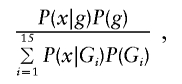where g represents the observed parent-offspring genotypic configuration, G represents the set of all 15 possible parent-offspring genotypic configurations (AA×AA→AA, AA×Aa→AA, … , aa×aa→aa), and x denotes the affected offspring phenotype. It is critical that the denominator is equal to the probability that a family has an affected offspring, which (in this specific case of parents with one offspring) is equal to the population prevalence, . To estimate the model parameters, it is necessary to specify the population prevalence and to constrain the denominator to be equal to it (this parameter is relatively robust to misspecification and is generally well known for common diseases). The parent-offspring genotype probabilities are simply functions of the population allele frequency and Mendelian transmission rules (e.g., the probability of observing AA×Aa→AA is p³q, where p and q are the allele frequencies, under the assumption of Hardy-Weinberg equilibrium and random mating).

Extending this to include parental phenotypes, for cases in which all trio offspring are affected but parents may or may not be affected, we use a likelihood based on the formula

where x_F,M,1 represents the vector of observed dichotomous phenotypes for the family, and x₁ denotes the affected offspring phenotype. By use of this framework, between and within components of association with the underlying construct of liability can be estimated, as for the quantitative variable case. In particular, we consider three tests: FAM_T, a 1-df association test of c=w=d versus c=w=d=0; FAM_W, a 1-df within-family association test of c=0, w=d versus c=w=d=0; and TDT_W, a 1-df within-family association test that is asymptotically equivalent to the standard TDT, w versus w=0. In this design, there is no power to estimate b, since there is no variation in offspring phenotype between families. In summary, FAM_T, a test of total association, is the most powerful but least robust to stratification; TDT_W is the least powerful but the most robust; and FAM_W is expected to represent a compromise in terms of power and robustness (as before, robust to stratification except if parents in the same family are stratified).

Simulations of Trios

To simulate the ascertained trio samples, unselected trio samples were first generated with a quantitative-trait score (representing liability). Either no QTL or a QTL accounting for ∼2% of the phenotypic variance of the continuous liability was generated, with equal allele frequencies. For both parents and offspring, a quantitative-trait threshold for affected status was set to give disease frequencies of 1%, 5%, 10%, or 20% (i.e., thresholds of 2.32635, 1.64485, 1.281551, or 0.841621 SDs above the mean). Trios with an unaffected offspring were excluded from subsequent analysis—the initial unselected number of trios was 10,000; 2,000; 1,000; or 500—to ensure that each simulated sample consisted of, on average, 100 ascertained trios, irrespective of disease frequency. The ascertained trio samples were then analyzed using the three qualitative trait models mentioned above: FAM_T, FAM_W, and TDT_W.

The residual variance was partitioned in one of two ways—in addition to a certain degree of nonshared variance (i.e., effects unique to each member of the trio), a shared component was generated that was either familial (shared between all three trio members) or polygenic (partially shared between a parent and offspring but not shared between parents). In each of the two sets of simulations, labeled “familial” and “polygenic,” the proportion of shared to nonshared variance was increased from 0% to 90%, in intervals of 10%. That is, a familial residual variance of 50% implies a residual correlation of 0.50 between parents and between parents and offspring; in contrast, a polygenic residual variance of 50% implies a parent-offspring correlation of 0.25 and no spousal correlation. Of course, familial and polygenic influences are not, in practice, mutually exclusive.

The utility of any method that incorporates qualitative parental phenotypes will clearly depend, to a large extent, on the presence of affected parents. Figure 1 shows the proportion of trios with at least one affected parent among the samples of trios ascertained for having an affected offspring. Also shown are the corresponding values of λ_O, the relative risk for parents of developing disease, given an affected offspring. In most cases, a reasonable proportion (∼20%) of trios contain at least one affected parent. If the disease frequency and the parent-offspring correlation are both low, then far fewer trios have at least one affected parent—one might expect the new methods to show little or no advantage in these scenarios. Of course, in the polygenic scenarios, the parent-offspring correlation will be lower for the same proportion of variance explained, as compared with the familial scenarios.

Figure 1.

Qualitative-trait simulations. A, Proportion of trios with at least one affected parent, with varying polygenic variance. B, λ_O, with varying polygenic variance. C, Proportion of trios with at least one affected parent, with varying familial variance. D, λ_O, with varying familial variance. Within each plot, the results are stratified by frequency of disease (1%, 5%, 10%, and 20%).

For simulations with no genetic effect, all methods show appropriate 5% type I error rates. For the cases in which a true genetic effect was simulated, the results for the standard TDT analysis will be first reported; these were not affected by the nature or degree of residual shared variance. The power of the TDT increases with decreasing disease frequency. This result is expected, since the gene acts as a QTL on the liability scale, and so a less frequent disease implicitly represents a higher threshold and therefore defines a more extreme group. The analytic power estimates for the standard TDT analysis are given by GPC (by use of the “TDT for threshold-selected quantitative traits” module) as ∼29%, 42%, 54%, and 75% for disease frequencies of 20%, 10%, 5%, and 1%, respectively (for the TDT_W test, the simulations also yielded average power estimates of 29%, 42%, 54%, and 75%, respectively).

With regard to the FAM_T and FAM_W tests, the results depend on the nature and degree of residual shared variance. In the polygenic scenarios, there is no strong trend toward greater power at higher levels of polygenic residual variance (results plotted in fig. 2). In contrast, the familial scenarios show a greater influence of the degree of residual shared variance, especially for rare diseases (results plotted in fig. 3).

Figure 2.

Qualitative-trait simulations. Power for the three tests (FAM_T, FAM_W, and TDT_W) are plotted against residual polygenic variance (X-axes) for the four disease frequencies (1%, 5%, 10%, and 20%).

Figure 3.

Qualitative-trait simulations. Power for the three tests (FAM_T, FAM_W, and TDT_W) are plotted against residual familial variance (X-axes) for the four disease frequencies (1%, 5%, 10%, and 20%).

It should be noted that the differences between figures 2 and 3 arise because of the higher average correlation between relatives in the familial, as opposed to polygenic, scenario, rather than because of the specific nature of that variation, per se (e.g., variation due to environmental factors as opposed to polygenes). This is simply because familial variance is completely shared among all three members of a trio, whereas polygenic variance is only 50% shared between parents and offspring and does not lead to any correlation between parents.

For the polygenic case, the new methods give a noticeable increase in power for common diseases. The effect is much less noticeable for rarer diseases (this is also apparent in terms of the average likelihood-ratio test statistic, and not just the power, which is approaching 100%, in any case).

For the familial cases, both FAM_T and FAM_W increase in power with increasing residual shared variance. This is analogous to the increase in power of the Fulker model within-family test with increasing residual sibling correlation (Sham et al. 2000). As expected, if the disease frequency and the residual correlation are both low, then FAM_T and FAM_W do not show any advantage relative to TDT_W. In these scenarios, we would not advocate the use of the parental phenotype models. In all other cases, however, the parental phenotype models show considerable gains in power. Since many complex human diseases are relatively common, show moderate-to-strong familial clustering, and are multifactorial (i.e., single loci will have small individual effects, and thus residual correlations are likely to be moderate to high), we can expect that the inclusion of parental phenotypes will often lead to an increase in power. Since disease frequency, parent-offspring, and parent-parent correlation in liability are likely to be known prior to starting any molecular genetic study, the question of whether parental phenotypes should or should not be collected can be decided in advance.

With respect to population stratification, the FAM_T and FAM_W tests show similar profiles to quantitative-trait tests E and C, respectively. That is, the FAM_W approach is robust to the between-family component of stratification, and the FAM_T is similar to a case-control design using unrelated individuals and so is not robust to any population-stratification effects. The present simulation results would suggest that, for ascertained trios, most of the power comes from the within-family component of association, and thus little would be lost in using the more robust FAM_W over FAM_T, in most circumstances. Of course, between-family stratification will act to increase the familial component of shared variance: this will increase the power of the FAM_W test, which is still robust to between family stratification (i.e., if allele frequency at the test locus also differs between strata).

Ascertaining Affected Parents

Whittaker and Lewis (1998) note that the power of the TDT might, in some circumstances, be improved by ascertainment by parental, as well as offspring, disease status. In particular, they suggest that ascertaining trios in which one parent is affected is often a practical way to increase power. We might also expect the new tests presented here that use parental phenotype information, to benefit from ascertainment of affected parents. In particular, the FAM_W test should perform particularly well when all trios have at least one affected parent (most trios will have only one affected parent, unless the disease is extremely common). To illustrate this point, we took a disease model used by Whittaker and Lewis (1998, multiplicative model 8 in table 2) that assumes a disease with 10% prevalence and a risk-allele frequency of 12.5% , with a genotypic relative risk of 2.9 (a relatively large effect). In all cases, we fix the sample size at 100 trios, and we use a type I error rate of 5×10^-8 to investigate power. The likelihood used in the FAM_W test has to be modified to account for the ascertainment by parental phenotype:

where x₁ denotes the affected offspring phenotype, and x_P denotes the affected parental phenotype (this revised test is hereafter denoted “FAM_W*”). All tests show appropriate type I error rates under the null hypothesis of no association in these conditions (for nominal rates of both 5% and 1%). When the disease-gene effect is simulated, we obtain estimates of power, as shown in table 3. Several interesting features emerge. First, by use of the standard TDT, the ascertainment of affected parents increases power only in some circumstances. If there is a high residual familial correlation (the r=0.6 scenario), then the ascertainment of trios with affected parents actually decreases power (from 36% to 17%). This seems intuitive: if family-wide environmental factors and polygenic factors other than the test locus account for the majority of within-family resemblance, then the cases of families with multiple affected members are more likely to be the result of causes other than the test locus (the influence of residual correlation was not explored by Whittaker and Lewis [1998]). Second, if the residual correlation is low, then ascertainment by parental disease status can increase power to some extent (from ∼30% to near 50%). Third, the use of the FAM_W* approach is more powerful, whether or not we ascertain by parental disease status. However, the most dramatic increase in power comes from the use of the FAM_W* test when we ascertain by parental disease status; power is 99% in all cases. This dramatic increase is not surprising when considered in light of figure 1—that is, since 100% of families now have at least one affected parent, the majority of families will contribute to the estimation of the d parameter.

Table 3.

Simulations Investigating the Impact on Power of the Ascertainment of Trios with an Affected Parent and an Affected Offspring^[Note]

	Result for ResidualFamilial Correlation Level
Test andStatus of Ascertainmentof Affected Parents	.0	.1	.6
TDTW:
Without ascertainment	.33	.35	.36
With ascertainment	.49	.49	.17
FAMW:
Without ascertainment	.46	.55	.60
FAMW*:
With ascertainment	.99	.99	.99

Note.— The disease model follows multiplicative model 8 of Whittaker and Lewis (1998, table 2). In all cases, 100 trios are used, and the ascertainment is for either only the offspring being affected or at least one parent being affected in addition to offspring. Note that the FAM_W* test is conditional on ascertaining an affected parent, as described in the text. Correct type I error rates are obtained for all tests under all scenarios when no genetic effect is simulated.

Summary

The incorporation of parental phenotypes can dramatically increase power, compared with the power of family-based tests that only use parental genotypes. We have presented a set of models for nuclear-family data that provide new tests offering similar efficiency to that of unrelated-individual designs, as well as a novel set of tests that offer a compromise in terms of efficiency and robustness—namely, tests that are robust only to the between-family component of stratification (see authors' Web site for information on scripts implementing the above-mentioned methods by use of the model-fitting package Mx). Naturally, standard within-family approaches can still be conducted within this framework if nuclear families have been sampled. In addition, there is some limited ability to detect departures from model assumptions, such as testing for stratification. The ability to strengthen or relax assumptions with regard to stratification, after the data have been collected, is a desirable feature, especially given the advent of other methods to detect stratification, such as those used by Pritchard et al. (2000).

This method can be easily extended to analyze multiallelic loci or phase-known haplotypes instead of biallelic genotypes, such that each allele and/or haplotype is analyzed one at a time versus all others. Alternatively, this approach can be incorporated into any framework that uses the basic between-within partitioning, to provide (for example) omnibus tests for multiallelic loci or haplotypes. Extension to phase-ambiguous haplotype analysis is also possible, although it will involve more work.

The more powerful tests of association proposed here have practical applications. Many studies involving trio collections have been completed, and, in some cases, it may be appropriate to reevaluate those studies with a more powerful test statistic. Furthermore, very large collections appropriate for family-based association tests are in the process of being collected for large-scale (and, perhaps soon, whole-genome) association studies. In some cases, there are genuine concerns about robustness, but, in many cases (such as in the study of common childhood diseases), families are collected simply because of convenience. If parents are recruited into studies for genotyping in the standard family-based approach, and if the cost of phenotyping is not prohibitively expensive, then these results suggest that to not collect and phenotype parents is often to miss an opportunity for considerable increases in power.

Appendix

For quantitative traits, a variance-components model under the assumption of multivariate normality describes the phenotypes in nuclear families, as discussed by Fulker et al. (1999) and Abecasis et al. (2000a). The vector of phenotypes, p∼N(μ,Σ), has expected values (as described in the main text) and a covariance matrix modeled by five unique parameters, distinguishing parent and offspring residual variances and covariances:

where V_P is the residual variance of the parental phenotypes, V_O is the residual variance of offspring phenotypes, C_P is the residual spousal covariance, C_O is the residual sibling covariance, and C_PO is the residual parent-offspring covariance. If there are multiple siblings in the family and identity-by-descent information is available, then this can be incorporated to model linkage and association simultaneously, which is directly analogous to the approach of Fulker et al. (1999) and that of QTDT software.

When parental phenotypes are entered as covariates, then the covariance matrix is simply

The same basic model is applied in analyzing dichotomous variables, within the context of a liability-threshold model. This model then applies to the continuous latent liability distribution.

References

- Abecasis GR, Cardon LR, Cookson WOC (2000a) A general test of association for quantitative traits in nuclear families. Am J Hum Genet 66:279–292 [DOI] [PMC free article] [PubMed] [Google Scholar]
- Abecasis GR, Cookson WOC, Cardon LR (2000b) Pedigree tests of transmission disequilibrium. Eur J Hum Genet 8:545–551 10.1038/sj.ejhg.5200494 [DOI] [PubMed] [Google Scholar]
- Fulker DW, Cherney SS, Sham PC, Hewitt JK (1999) Combined linkage and association sib-pair analysis for quantitative traits. Am J Hum Genet 64:259–267 [DOI] [PMC free article] [PubMed] [Google Scholar]
- Pritchard JK, Stephens M, Donnelly P (2000) Inference of population structure using multilocus genotype data. Genetics 155:945–959 [DOI] [PMC free article] [PubMed] [Google Scholar]
- Purcell S, Cherny SS, Sham PC (2003) Genetic Power Calculator: design of linkage and association genetic mapping studies of complex traits. Bioinformatics 19:149–150 10.1093/bioinformatics/19.1.149 [DOI] [PubMed] [Google Scholar]
- Purcell S, Sham PC. Properties of structured association approaches to population stratification. Hum Hered (in press) [DOI] [PubMed] [Google Scholar]
- Sham PC, Cherny SS, Purcell S, Hewitt JK (2000) Power of linkage versus association analysis of quantitative traits, by use of variance-components models, for sibship data. Am J Hum Genet 66:1616–1630 [DOI] [PMC free article] [PubMed] [Google Scholar]
- Spielman RS, McGinnis RE, Ewens WJ (1993) The transmission test for linkage disequilibrium: the insulin gene region and insulin-dependent diabetes mellitus (IDDM). Am J Hum Genet 52:506–516 [PMC free article] [PubMed] [Google Scholar]
- Whittaker JC, Lewis CM (1998) The effect of family structure on linkage tests using allelic association. Am J Hum Genet 63:889–897 [DOI] [PMC free article] [PubMed] [Google Scholar]