Rapid Simulation of P Values for Product Methods and Multiple-Testing Adjustment in Association Studies

Abstract

A major aim of association studies is the identification of polymorphisms (usually SNPs) associated with a trait. Tests of association may be based on individual SNPs or on sets of neighboring SNPs, by use of (for example) a product P value method or Hotelling’s T test. Linkage disequilibrium, the nonindependence of SNPs in physical proximity, causes problems for all these tests. First, multiple-testing correction for individual-SNP tests or for multilocus tests either leads to conservative P values (if Bonferroni correction is used) or is computationally expensive (if permutation is used). Second, calculation of product P values usually requires permutation. Here, we present the direct simulation approach (DSA), a method that accurately approximates P values obtained by permutation but is much faster. It may be used whenever tests are based on score statistics—for example, with Armitage’s trend test or its multivariate analogue. The DSA can be used with binary, continuous, or count traits and allows adjustment for covariates. We demonstrate the accuracy of the DSA on real and simulated data and illustrate how it might be used in the analysis of a whole-genome association study.

Introduction

Association studies are commonly used to test for association between some trait (e.g., disease) and SNPs within a candidate gene or region. These candidate genes or regions are chosen because of their known biological function or because they have been identified as interesting in linkage studies. As the cost of SNP genotyping diminishes, whole-genome association studies become ever more feasible.

Many methods are available for testing association between genotype and trait. Each SNP may be tested individually, or information from a set of neighboring SNPs may be combined. The latter approach may be more powerful, since a causal locus may be associated with not just one SNP but with several nearby SNPs. When information from a set of SNPs is combined, the test may be based on haplotype scoring (Schaid et al. 2002; Fan and Knapp 2003) or on locus scoring (Xiong et al. 2002; Chapman et al. 2003). Haplotype scoring means that several SNPs are treated together as a multiallelic marker and the trait is regressed on an individual’s two haplotypes at this marker. As haplotypes are usually not observed, they must be imputed by use of (for example) an expectation-maximization (EM) algorithm. Locus scoring means that there is a covariate for each SNP, indicating the number of variant alleles carried by an individual at that SNP, and that the trait is regressed on this set of covariates. In this case, there is no need to impute the haplotypes.

In this article, we consider tests based on individual SNPs or on locus scoring of SNP sets. There is a lively debate about whether tests based on haplotype scoring or those based on locus scoring are more powerful. This article does not aim to provide evidence to support either position. Here, we note only that a number of studies have found evidence in favor of locus scoring—for example, studies by Long and Langley (1999), Kaplan and Morris (2001), and Chapman et al. (2003). Zaykin et al. (2002a) found that tests based on haplotypes were more powerful, but they only compared them with tests based on individual SNPs, rather than tests based on locus scoring of the corresponding sets of SNPs.

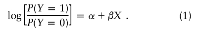
A popular test for association between a binary trait, Y, and an individual SNP is Armitage’s test for trend (Sasieni 1997). Under Hardy-Weinberg equilibrium, this test is asymptotically equivalent to the allele-counting test but has the advantage that it retains the correct type I error rate when Hardy-Weinberg equilibrium is violated (Sasieni 1997). Label the two alleles at the SNP as wild type and variant (the choice of assignment is unimportant), and assign to the trait the two possible values of 0 and 1. For example, in a case-control study, 1 would denote a case, and 0 would denote a control. Let X denote the locus score for an individual—that is, the number of variant alleles (0, 1, or 2) carried by that individual. Consider the logistic regression of Y on X:

Armitage’s test is the score test for the null hypothesis that β=0. Suppose that α+βX in equation (1) is replaced by α+β₁X₁+…+β_JX_J, where X_j is the locus score at SNP j (j=1,…,J). Then, a generalization of Armitage’s test to J SNPs is the score test of the null hypothesis that β₁=…=β_J=0. This multilocus Armitage (MLA) test is closely related to Hotelling’s T test (see the “Score Statistics for a Class of GLMs” section below). Alternatives to the MLA test or to Hotelling’s T test are Fisher’s product P value method (FPM) (Fisher 1932), the truncated product method (TPM) of Zaykin et al. (2002b), and the rank TPM of Dudbridge and Koeleman (2003). In these methods, a P value for each individual SNP is calculated (e.g., by use of Armitage’s test), and then a combined test statistic is obtained by multiplying together either all the P values (in the FPM), just those below some significance threshold (in the TPM), or the R smallest P values (in the rank TPM). If the individual tests are independent, then exact analytic expressions exist for the significance of the combined test statistic. Otherwise, Zaykin et al. (2003b) and Dudbridge and Koeleman (2003) propose a number of approximate methods and propose permutation as an exact (apart from Monte Carlo error) method.

Armitage’s test and its MLA test generalization have the advantage that the null distributions of their test statistics are known, and hence P values can be calculated analytically. However, when multiple tests are performed, these P values are usually adjusted to take this into account. The most common approach is to focus on the minimum P value and to evaluate the probability that a value as small as this would be observed if all the null hypotheses were true. Two simple ways to do this are the Bonferroni and Šidák methods (Šidák 1967), but these lack power when the test statistics are positively correlated, as is the case with SNPs in linkage disequilibrium (LD). In this situation, efficient multiple-testing correction requires permutation.

So, permutation may be required for product P value methods and also for efficient multiple-testing correction of Armitage and MLA tests. The use of permutation can be expensive in terms of computer time, especially if the number of subjects in the study is large. In this article, we introduce an alternative method, the direct simulation approach (DSA). This involves deriving the multivariate normal asymptotic null joint distribution of the test statistics and sampling directly from it. The DSA is much faster than permutation, and the computational requirement is independent of the number of subjects. It may be used whenever the individual tests are score tests. These include not only tests for binary responses but also tests for continuous and count responses.

In the next section, we derive the form of the score statistic for a class of generalized linear models (GLMs). The “Minimum and Product P Values” section below contains a description of the minimum P value and product P value methods and a suitable permutation algorithm for calculating them. The DSA is introduced in the “DSA” section and is compared with the permutation algorithm. Illustrative applications of the DSA follow in the “Applications to Minimum and Product P Values” and “DSA in a Whole-Genome Association Study” sections. Finally, there is the “Discussion” section.

Score Statistics for a Class of GLMs

Much of what follows in the section below is adapted from Schaid et al. (2002). Let Y denote a measured trait, X_e a vector of measured environmental factors plus unity as the first element, and X_g a vector of locus scores—that is, the lth element of X_g is the number of variant alleles (0, 1, or 2) carried by the individual at SNP l. We assume the relation between trait Y and covariates Z^T=(X^T_e, X^T_g) can be expressed as a GLM for exponential family data. Let η=X^T_eα+X^T_gβ=Z^Tγ, where γ^T=(α^T,β^T). The likelihood of Y, given Z, can be written as

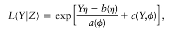where a, b, and c are known functions, and where φ is the dispersion parameter. Let f denote the link function, so that the expected trait value, given the covariates, is . Parameter vector α describes the influence of environmental factors on the trait, and includes an intercept term. Parameter β describes the effect of genotype on the trait. No association between trait and genotype corresponds to β=0.

Let X_ei, X_gi, Z_i, and Y_i denote the values of X_e, X_g, Z, and Y for subject i (i=1,…,N), and let L_i be the subject's likelihood contribution. As Schaid et al. (2002) show, the score statistic for genetic markers, X_g, adjusted for environmental covariates, X_e, is

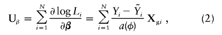where , the fitted value for subject i when β=0, is obtained by regressing Y on just X_e to obtain the maximum-likelihood estimate of α and then setting .

The variance of U_β under the null hypothesis (H₀) that β=0, with the adjustment for the environmental covariates taken into account, is V_β=V_ββ-V_βαV^-1_ααV_αβ, where V_ij is the appropriate submatrix of matrix V(U_γ):

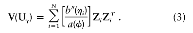Without environmental covariates, α consists of only an intercept term, and the variance simplifies to

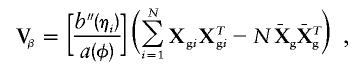where . Under H₀,U_β is asymptotically distributed multivariate normal (McCullagh and Nelder 1989), with mean zero and variance V_β:

This is an asymptotic result, which requires that the dimension of Z (i.e., the number of environmental factors, including the intercept, plus the number of SNPs) be small in comparison with the number of subjects, N. In most of the applications reported in the “Applications to Minimum and Product P Values” and “DSA in a Whole-Genome Association Study” sections, N is ∼10 times the dimension of Z. It follows from equation (4) that the score test statistic, T=U^T_βV^-1_βU_β, is asymptotically χ² distributed with degrees of freedom equal to the length of vector X_g. If matrix V_β is not of full rank, V^-1_β is replaced by its generalized inverse, and the number of degrees of freedom is now equal to the rank of V_β.

Schaid et al. (2002) give the form of , a(φ), and b^′′(η) for GLMs based on Gaussian, binomial, and Poisson distributions. For a binary trait and no covariates, , a(φ)=1, and , and it is straightforward to show that T is the same as the test statistic described by Chapman et al. (2003). It is also closely related to Hotelling’s T test (as used by, e.g., Xiong et al. [2002] and Fan and Knapp [2003]), the difference being that, in Hotelling’s test, V_β is the weighted mean of the variance of X_g estimated in the cases and controls separately. In the special case in which X_g is univariate, the score test reduces to Armitage’s test (strictly, Armitage’s trend test statistic is T[N-1]/N).

Minimum and Product P Values

Suppose L null hypotheses, H₀₁,…,H_0L, are being tested by use of score tests. Let T₁,…,T_L denote the respective score test statistics, and let t₁,…,t_L denote the corresponding observed values. Under the composite null hypothesis H₀=∩^L_k=1H_0l, the marginal distributions of T₁,…,T_L are χ² with known degrees of freedom, d₁,…,d_L. Let random variable P_l denote the P value for T_l —that is, P_l=1-F_dl(T_l), where F_dl is the distribution function of the χ²_dl distribution. Let p_l be the observed value of P_l. Hence, p_l=P(T_l⩾t_l|H_0l). Let G=G(P₁,…,G_L) be some function, and let g=G(p₁,…,p_L) be its observed value. Suppose we wish to calculate Q=P(G⩽g|H₀). Here are four examples of G that could be of interest:

• 1. Let P₍₁₎⩽…⩽P_(L) denote the ordered P values. If G(P₁,…,P_L)=P₍₁₎, then Q is the minimum P value, P_min. Note that we might also want to calculate G_l(P₁,…,P_L)=P_(l) for all l=2,…,L. This would allow the null hypotheses H₀₁,…,H_0L to be tested individually (Westfall et al. 2001).
• 2. If G(P₁,…,P_L)=l=1LP_l, then Q is the FPM P value, P_Fish.
• 3. If G(P₁,…,P_L)=l=1LP_lI(P_l⩽τ), where I is the indicator function, then Q is the TPM P value with threshold τ, P_trunc(τ).
• 4. If G(P₁,…,P_L)=l=1RP_(l), then Q is the rank TPM P value based on the R smallest P values, P_rank(R).

When the L tests are independent, formulae for these P values are available (Zaykin et al. 2002b; Dudbridge and Koeleman 2003). However, when the test statistics are correlated, these tests do not apply. The Bonferroni method provides a formula for P_min when tests may be dependent, but this is an upper bound and is conservative when tests are positively correlated. Zaykin et al. (2002b) show how to calculate P_trunc(τ) and P_Fish when the correlation matrix of the P values is known, but typically this will not be the case. Dudbridge and Koeleman (2003) describe a method of estimating P_trunc(τ), P_rank(R), and P_Fish, but this method is untested and, anyway, requires the calculation of P_min by permutation. Nyholt (2004) describes a simple way of estimating P_min using a Šidák correction based on an effective number of independent tests estimated from the correlation matrix of imputed haplotypes. However, the performance of this method has not been tested properly. Permutation remains the most reliable way of calculating P_min, P_trunc(τ), P_rank(R), and P_Fish.

An appropriate permutation algorithm is described by Schaid et al. (2002). Although not explicitly stated by Schaid et al., the algorithm requires the assumption that X_e and X_g are independent. Under H₀, the trait value, Y, and the genotype, X_g, are independent, so any permutation of the N X_g values among the N subjects is, a priori, equally probable. The vector Y is permuted B times and, for permutation b (b=1,…,B), the P values, , are calculated and, from these, . An unbiased estimator of Q is

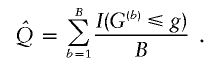DSA

Suppose tests T₁,…,T_L depend on a total of M SNPs. For example, for each l (l=1,…,L), T_l might be Armitage’s test statistic for SNP l, and M=L. Let E be the dimension of X_e—that is, the number of environmental factors (including the intercept). Suppose M+E is small compared with N—for example, E+M⩽N/10 (below, we discuss what to do otherwise). Equation (2) shows that, to calculate the score statistics required by T₁,…,T_L, it is necessary to evaluate the sum of over the N individuals. This must be done for each permutation. The variance of the score statistic is independent of Y (see eq. [3]) and is calculated only once. Thus, the computation required is proportional to N, the number of subjects in the study. The DSA, which we now describe, avoids the need to perform these summations at each permutation, and its computational requirement is independent of N. It therefore can be much faster than permutation, especially when N is large.

Let U_β(+) and V_β(+) denote the score-statistic vector and its variance matrix for the whole set of M SNPs. Let U_β(l) and V_β(l) denote the corresponding entities for just the SNPs involved in test T_l, so that T_l=U^T_β(l)V^-1_β(l)U_β(l). Equation (4) shows that, under the null hypothesis that none of the M SNPs are associated with the trait, U_β(+) is approximately distributed N(0,V_β(+)). Since, for each l, U_β(l) is a subvector of U_β(+), its distribution is a marginal distribution of the distribution of U_β(+). Therefore, equation (4) implies the null joint distribution of (U^T_β(1),…,U^T_β(L)). So, to obtain B samples from the null joint distribution of (T₁,…,T_L), it is not necessary to permute vector Y B times and to calculate U_β(l),…,U_β(L) each time by use of equation (2). Instead, one can directly simulate B U_β(+) vectors independently from an N(0,V_β) distribution and obtain B sets of vectors U_β(l),…,U_β(L) as the appropriate subvectors. The remainder of the algorithm—that is, the calculation of t^(b)₁,…,t^(b)_L; of ; and finally of G^(b)—remains unchanged.

If each of the L tests is based on just one SNP (e.g., Armitage tests) and so U_β(+)=(U_β(1),…,U_β(L)), then the algorithm can be accelerated slightly by noting that, in this case, . Since it follows from equation (4) that V^-1/2_β(+)U_β(+)∼N(0,C) asymptotically, where C is the correlation matrix corresponding to variance matrix V_β(+), the B vectors can be directly simulated from an N(0,C) distribution.

When M+E is not small in comparison with N (e.g., M+E>N/10), the normal approximation of equation (4) may not be so good. However, if the P value of interest is P_min, then this need not be a problem. In this case, the M SNPs may be divided into K blocks (e.g., of size ⩽N/10-E), and the score vector may be simulated for each block independently. To be more precise, denote the simulated score vector for block k (k=1,…,K) as U_β(+)k. One would simulate U_β(+)k for each block k independently and then would calculate the whole vector of test statistics, (T^(b)₁,…,T^(b)_L), from U_β(+)1,…,U_β(+)K. An example is given in the “DSA in a Whole-Genome Association Study” section. This amounts to the assumption of independence between pairs of SNPs in different blocks, which will cause some loss of power. However, since most of the dependence structure between SNPs—that is, the structure within blocks—is being captured, the loss should be small. If haplotype block structure is observed in the region being analyzed, then the divisions between blocks of SNPs can be chosen to coincide with haplotype block boundaries.

Note that the DSA requires complete data to calculate V_β. Missing genotypes must be imputed. Provided that the imputation is done in a way that does not use information on the trait values of the individuals, the type I error rate will not be inflated. One method is to impute missing values as their posterior expectations, given the observed genotype data (under H₀). This requires haplotype frequencies. As these are usually not known, an EM algorithm could be used to estimate them. Multilocus score tests (and Hotelling’s test) require complete data, and so imputation must be performed regardless of whether permutation or the DSA is used. However, when T₁,…,T_L are univariate (individual SNP) tests, the DSA has the disadvantage that it requires imputation, whereas permutation does not. As the EM algorithm may require considerable computational time, we use a simpler and much faster linear regression procedure. For each j (j=1,…,M) in turn, the locus score at SNP j is regressed on the locus scores at neighboring SNPs, and missing scores at SNP j are imputed as their fitted values. There is flexibility in the choice of neighboring loci on which to base imputation of a target SNP. We recommend either the use of all other genotyped SNPs in the same gene or haplotype block as the target SNP or the use of all genotyped SNPs whose LD with it exceeds a certain threshold. Provided the ability (measured by R²) of the chosen set to predict the target SNP is high, the addition of further markers to the set should make little difference to the imputed values.

In the two sections that follow, we illustrate several uses of the DSA and compare its performance withpermutation. Analyses were performed on a Linux workstation with a 1.6-GHz Advanced Micro Devices (AMD) processor using the software R, and all code was optimized to make full use of the latter’s powerful matrix algebra computation (see Max Planck Institute of Psychiatry Web site for R code).

Applications to Minimum and Product P Values

The Munich Anti-Depressant Drug Response Study (MARS) is a longitudinal study of depressed patients that investigates associations between candidate genes and responses to treatment with antidepressant drugs (Binder et al. 2004). Here, we analyze a total of 31 SNPs in eight genes, using Armitage’s test for each individual SNP and using the MLA test, FPM, and TPM for each whole gene. The tested trait was response to treatment at 2 wk. Of 227 patients, 51% responded.

Both the DSA and permutation were used to calculate P_min, P_Fish, and P_trunc(0.05). The results in table 1 are based on B=50,000 permutations/simulations, except for the result for FKBP5, which was highly significant and thus required a larger number; we used B=200,000. Usually, <50,000 permutations would be used for the nonsignificant genes, but we wanted to reduce the Monte Carlo variance for the comparison of P values calculated by the DSA and permutation. In table 1, the columns labeled “DSA” and “PerI” contain P values calculated by the DSA and permutation, respectively, after missing values were imputed. The columns labeled “Perm” have P values for permutation with missing values left as missing (1.7% of genotypes were missing). The last two columns of the table give P values for the MLA test, calculated by use of both the usual asymptotic χ² assumption (the column labeled “Asym”) and permutation.

Table 1.

P Values Obtained for Eight Genes by Use of the Minimum P Value Method, FPM, TPM, and MLA Test

	P Value by Use of
	MPMa(Pmin)			FPM(PFish)			TPM(Ptrunc(0.05))			MLA
Gene	DSAb	PerIc	Permd	DSAb	PerIc	Permd	DSAb	PerIc	Permd	Asyme	PerIc
AVP	.910	.936	.939	.884	.881	.880	1.000	1.000	1.000	.944	.946
BAG1	.377	.384	.415	.252	.255	.272	1.000	1.000	1.000	.277	.282
CRH	.133	.131	.128	.236	.235	.230	1.000	1.000	.128	.206	.206
FKBP4	.795	.815	.818	.920	.924	.924	1.000	1.000	1.000	.877	.877
FKBP5	.004	.003	.004	.001	.001	.001	.001	.001	.001	.016	.012
NR3C1	.795	.789	.818	.824	.820	.828	1.000	1.000	1.000	.393	.388
TEBP	.888	.872	.871	.758	.756	.746	1.000	1.000	1.000	.744	.765
STUB1	.064	.070	.070	.110	.114	.112	.064	.070	.070	.098	.097

^aMPM = minimum P value method.

^bCalculated using the DSA with imputation of missing genotypes.

^cCalculated using permutation with imputation of missing genotypes.

^dCalculated using permutation without imputation.

^eCalculated using the asymptotic null distribution with imputation.

P values calculated by the DSA and permutation after imputation of missing values are very similar. The differences are no greater than those between P values for the MLA test calculated using the asymptotic assumption versus permutation. The effect of imputed missing data is observed by comparing columns labeled “PerI” with those labeled “Perm.” The pairs of P values are similar. For example, for FKBP5, P_min, P_Fish, and P_trunc(0.05) are .0043, .0010, and .0008, respectively, without imputation and are .0033, .0009, and .0007, respectively, with imputation.

The smallest raw P value observed for the 31 SNPs was .00162 (in FKBP5), which makes the Bonferroni-corrected P value .00162×31=.050. This compares with a P value of .031 for permutation, showing that calculating P_min by permutation can be worthwhile. The use of the FPM or TPM yields even more significant P values for FKBP5: P_Fish and P_trunc(0.05) are ∼5 times smaller than P_min. This is because not just one but three of the four SNPs in FKBP5 have small P values. The MLA test applied to FKBP5 yields a much less significant P value: P=.016 by use of the asymptotic assumption, and P=.012 by use of permutation. After Bonferroni correction for the fact that eight genes have been tested, this becomes nonsignificant: P=.016×8=.13.

The time required for this analysis was 62 s for the DSA, compared with 650 s for the same analysis using permutation without imputation—a reduction of 90%. After it was established that FKBP5 was significantly associated with response to treatment, a further 29 SNPs within and near this gene were typed in an effort to fine map the causal locus (Binder et al. 2004). Using the complete set of 33 SNPs, we compared P values obtained by the DSA with those obtained by permutation. B=200,000 permutations/simulations were performed. This is a challenging data set, since the spacing between SNPs is quite small (average spacing 9 kb) and the ratio of the number of subjects to the number of parameters (34) is only 6.7. Thus, the multivariate normal approximation of the score vector (eq. [4]) may not be so good. The values of P_min from the DSA, permutation with imputation, and permutation without imputation were .029, .024, and .036, respectively. The Bonferroni-corrected P value was .070, so the result of permutation or the DSA is a noticeable improvement on this value. The P_Fish values were .0031, .0027, and .0036 for the DSA, permutation with imputation, and permutation without imputation, respectively. The P_trunc(0.05) values were .0055, .0048, and .0046 for the three methods. Thus, even for this challenging data set, the performance of the DSA is encouraging. The time required was 44 s for the DSA, compared with 640 s for permutation. The MLA test was also performed on this data set but was found to yield a much less significant result than the minimum P value method, FPM, or TPM, and, again, the P value obtained using the asymptotic assumption (P=.173) was greater than that obtained using permutation (P=.141).

A more extensive evaluation of the DSA was performed using data simulated by the HaploBlock version 1.2 software (Greenspan and Geiger 2004). An original founding population size of 20 individuals was assumed. This expanded with an exponential growth rate of 1.1, reaching 50,000 in ∼80 generations, and then drifted for a further 170 generations. From this population, 2,000 haplotypes, each containing 100 SNPs with an average intermarker spacing of 2 kb, were sampled, and the haplotypes were paired at random to form genotypes for 1,000 individuals. Two hundred sets of case-control labels for the 1,000 individuals were simulated, so that, in each set, 500 were cases and 500 were controls. Of these sets, 100 were simulated under the null hypothesis of no association within the region, and 100 were simulated under the assumption that SNP number 20 was a causal locus for disease. For these latter 100 sets, the probabilities of being a case were proportional to 1, 1.5, and 2 for persons carrying 0, 1, or 2 variant alleles, respectively, at SNP 20. This SNP was then removed from the set of markers. By this procedure, 200 data sets were created, each having the same LD structure. The whole procedure was repeated four times—each time by starting with a different random founding population, expanding it exponentially, sampling 2,000 haplotypes, and finally generating 200 sets of case-control labels—to produce a total of five groups of 200 data sets, each group having a different LD structure.

The minimum P value method, FPM, and TPM were applied to each of the 1,000 simulated data sets, by use of both permutation and the DSA, to evaluate the accuracy of the DSA as an approximation to permutation. B=50,000 permutations/simulations were performed, which required 30 s per data set for the DSA and 520 s for permutation. Let P_perm denote a P value obtained by permutation and P_DSA denote the corresponding value from the DSA. Define D=100%×(P_DSA-P_perm)/P_perm. Mean D over all 1,000 data sets was 3%, 6%, and 4% for the minimum, FPM, and TPM P values, respectively. Thus, the DSA seems slightly conservative. Mean |D| was 7%, 9%, and 8% for the minimum, FPM, and TPM P values, respectively. The accuracy of the DSA approximation for small P values is of particular interest. For P values between .001 and .005, mean D was 0%, 9%, and 8% for the three methods, and mean |D| was 0%, 13%, and 14%. P values <.001 were not examined, since, with Monte Carlo error, these are less precise estimates.

Finally, by use of the 500 data sets simulated under the alternative hypothesis, the powers of the minimum P value method, FPM, and TPM were examined. With a type I error rate of 5%, the power of the minimum P value method was 67%. The powers of the FPM and TPM were higher—75% and 74%, respectively—which again demonstrates the potential of these methods. The improvement in power was even greater for type I error rates of 1% and 0.1%.

DSA in a Whole-Genome Association Study

As the cost of genotyping decreases, whole-genome association studies are beginning to become feasible. In such a study, SNPs would be genotyped throughout the genome with an intermarker spacing of (for example) 5 kb or 10 kb. These SNPs may or may not have been selected as haplotype-tagging SNPs (Johnson et al. 2001). We now illustrate how the DSA could be used in a variety of ways to accelerate the analysis of data from such a study. We consider a 10-Mb segment of chromosome, but the analysis could, in principle, be scaled up to cover the whole genome.

By use of HaploBlock version 1.2, a 10-Mb map with ∼10-kb marker spacing and otherwise the same parameters given in the “Applications to Minimum and Product P Values” section was simulated. Genotypes for 1,000 individuals at 1,035 SNPs were generated, 500 were randomly assigned to be cases, and 500 were assigned to be controls. SNP 844 was chosen as a causal locus, and the probabilities of being assigned as a case were proportional to 1, 2, and 3 for persons carrying 0, 1, or 2 variant alleles, respectively, at this SNP. SNP 844 was then removed from the data set.

Individual SNPs were tested using Armitage’s test. Figure 1 (top panel) shows the resulting P values. The minimum P value is 2.7×10^-5 at SNP 848, which, after Bonferroni correction for 1,034 tests, becomes .028. By use of permutation, the adjusted minimum P value was .026 (B=100,000). The DSA approximation of this was P=.023. Note that, in using the DSA, the 1,034 SNPs were partitioned into 10 blocks of ∼103 SNPs each, so that N was large compared with the number of SNPs in a block. Block 1 consisted of SNPs 1–103, block 2 consisted of SNPs 104–206, and so forth, with block 10 containing SNPs 928–1,034. For each replicate b (b=1,…,B), score vectors U_β(+)1,…,U_β(+)10, each of length 103 (except for block 10, length 107), were generated independently from their appropriate multivariate normal null distributions (of dimension 103 or 107). Then, the test statistics T^(b)₁,…,T^(b)₁₀₃ were calculated from U_β(+)1, the statistics T^(b)₁₀₄,…,T^(b)₂₀₆ from U_β(+)2, and so forth.

Figure 1.

For 1,034 SNPs in the 10-Mb region, the P values for individual-SNP Armitage tests (top), for the TPM on a window of 11 SNPs (middle), and for MLA tests on a window of 11 SNPs (bottom). Dotted lines indicate the Bonferroni-adjusted 5% and 1% significance thresholds.

Zaykin et al. (2002b) proposed the use of the TPM to analyze such data. They simulated case-control data for a 143-cM map with 2,610 SNPs and tested each SNP for association with disease by use of Fisher’s exact test. After Bonferroni correction, none was significant at the 1% level. The TPM was then used to combine the P value from each SNP with those of its neighboring 10 SNPs (i.e., 5 SNPs on either side). The minimum TPM P value, after Bonferroni correction, was well below .01, showing the potential benefits of combining evidence from neighboring SNPs. However, Zaykin et al. (2002b) calculated the TPM P values under the assumption that the correlation matrix of the P values for a window of 11 neighboring SNPs is constant across the entire 2,610 SNPs, which is somewhat optimistic.

We used the same approach of combining the P values of 11 neighboring SNPs, using the TPM on our simulated data. In a real application, one might adopt a more sophisticated way of choosing sets of SNPs to combine, making use of haplotype block structure. Instead of assuming a constant correlation matrix for P values of adjacent SNPs, as Zaykin et al. (2002b) did, we used the DSA. Again, we divided the 1,034 SNPs into 10 blocks. In this case, however, each test depends on a window of 11 neighboring SNPs and, because windows overlap, the blocks must also overlap. Thus, block 1 consisted of SNPs 1–108, block 2 of SNPs 99–211, block 3 of SNPs 202–314, and so forth. That is, the blocks were the same as before, but with an additional five SNPs included on either side. Score vectors U_β(+)1,…,U_β(+)10, each of length 113 (except for block 1 [length 108] and block 10 [length 112]), were generated independently from their multivariate normal null distributions. Then, test statistics T^(b)₁,…,T^(b)₁₀₃, for windows centered on SNPs 1–103, were calculated from block 1; T^(b)₁₀₄,…,T^(b)₂₀₆ were calculated from block 2; and so forth.

Figure 1 (middle panel) shows the resulting P values. The minimum TPM P value (obtained using B=5×10⁶) was 1.0×10^-5 at SNP 849 (and it was 1.1×10^-5 when permutation was used). Adjustment of this minimum TPM P value by use of the Bonferroni method yielded P=.011. This adjustment ignores the correlation between TPM P values, which is high in this situation because of the use of overlapping windows. Power is gained by taking this correlation into account, which can be done using the algorithm of Ge et al. (2003). This yielded an adjusted minimum TPM P value of .0043.

Finally, the MLA test was applied to the same windows, and figure 1 (bottom panel) shows the P values. The minimum MLA P value was 1.9×10^-7 at SNP 847. Bonferroni adjustment yielded P=2.0×10^-4. Again, the MLA tests are correlated, and power is gained by taking this correlation into account. Multiple-testing adjustment by use of the DSA with B=10⁶ yielded P=8.1×10^-5 (P=5.4×10^-5 by use of permutation).

In conclusion, for this data set, the combining of P values from neighboring SNPs is certainly worthwhile, and the MLA test gives a more significant result than the TPM. The difference between multiple-testing–adjusted TPM or MLA P values calculated using the algorithm of Ge et al. (2003) or the DSA and those calculated using Bonferroni’s method shows the benefit of the more powerful methods.

The DSA required about 5% of the time required by permutation in most of these analyses. The exception was the multiple-testing adjustment of the MLA test, in which the DSA required slightly <20% of the time required for permutation. The reason for this difference is that the MLA test involves matrix multiplication to calculate T_l=U^T_β(l)V^-1_β(l)U_β(l), and this requires an increasingly nonnegligible computation time as the dimension of U_β (11, in this application) increases.

Discussion

The DSA has been demonstrated to be a good approximation to permutation, but much faster. In particular, it is no less accurate than the use of the asymptotic null distribution to calculate the P value of the MLA test, which is done by both Chapman et al. (2003) and Schaid et al. (2002). Also, given the very close relation between the MLA test and Hotelling’s T test, it is likely to be no worse than the use of the asymptotic null distribution for Hotelling’s test. In the applications reported in the present study, the DSA requires 5%–20% of the time required for permutation.

There are possibilities for reducing the computational time further. First, importance sampling could be used. The DSA amounts to evaluating a probability (the P value) by Monte Carlo integration. Importance sampling is another Monte Carlo integration approach, which might require fewer simulations of the score vector. A second way to reduce the number of simulations would be to fit a parametric distribution to the simulated P values (Dudbridge and Koeleman 2004).

When the null distributions of T₁,…,T_L are the same, a third way to reduce the computational time would be to work directly with these test statistics rather than convert them into P values. For multiple-testing adjustment of minimum P values, the use of G=-max{T₁,…,T_L} gives the same P_min as the use of G=P₍₁₎. In combining tests, test statistics may be summed rather than having their P values multiplied (Neuhaüser 2003). In cases in which the null distributions of T₁,…,T_L are χ²₂, the summing of test statistics and the multiplying of P values yield the same P_Fish and P_trunc(τ). In other cases, the final P values will be different, but the test will be no less valid. As Zaykin et al. (2002b) note, there is no uniformly most powerful way to combine P values. For the FKBP5 data, summing the Armitage test statistics rather than multiplying P values reduced the computational time for the DSA by 16% and gave very similar results. In fact, when the SNPs are in linkage equilibrium, the MLA test statistic for a set of SNPs is approximately equal to the sum of the Armitage test statistics for the individual SNPs. This is because V_β is approximately diagonal, and so T=U^T_βV^-1_βU_β≃U_β(1)V^-1_β(1)U_β(1)+…+U_β(L)V^-1_β(L)U_β(L).

For association studies, the MLA test has the advantage that the asymptotic null distribution of the test statistic is known, and so P values can be calculated analytically. However, as Chapman et al. (2003) showed, its power begins to diminish as the density of SNPs increases beyond a certain unknown threshold. This is because the number of degrees of freedom of the test continues to increase, whereas the ability of the marker SNPs to predict the SNP at the causal locus tends toward a limit (or reaches it, if the marker set contains the causal SNP). This may be the reason why the significance of the MLA test, when applied to the FKBP5 fine-mapping set, is much less than that of the minimum P value method, FPM, and TPM. In fact, the context in which Chapman et al. (2003) propose the MLA test is one of haplotype-tagging SNPs, in which the tagging SNPs have been selected to minimize redundancy in the set of markers for predicting the genotype at a causal locus. The FPM and TPM do not have this drawback, and the TPM may have an advantage when only a few of the SNPs in the set are associated with the trait or when some SNPs are more strongly associated than others (Zaykin et al. 2002b). On the other hand, they require permutation, the DSA, or a crude approximation to obtain the P value and, if the set of SNPs being tested contains a subset of SNPs which have higher LD with each other than the average LD in the set, then this subset may dominate the test statistic, which means that the power to detect association with SNPs inside the subset will be high but, for SNPs outside the subset, power will be lacking. Thus, neither the MLA test (or the closely related Hotelling’s test) nor product methods are uniformly better than the other.

The principle of sampling directly from the asymptotic null joint distribution of a set of test statistics is not limited to trend-type tests, or even to GLMs. Within the context of the class of GLMs described in the present study, it would be straightforward to allow for dominance by replacing X_g, the covariate denoting the number of variant alleles carried, with two indicator variables; one of which is given the value 1 when one variant allele is carried, and the other is given the value 1 when two are carried. Multiallelic markers could also be incorporated easily by replacing X_g with (X_g1,…,X_gA), where X_ga denotes the number of copies of allele a (a=1,…,A) that are carried. This would yield the multiallelic trend test (Czika and Weir 2004). Beyond GLMs, many types of score tests could be treated in a similar way. For example, concerns about the vulnerability of population case-control studies to false positives due to population admixture and cryptic relatedness led to the popularity of family-based studies and the transmission/disequilibrium test (TDT) (Spielman et al. 1993). If phase is known, the joint null distribution for a set of TDTs is straightforward to derive (see the appendix).

A reviewer of the present work drew our attention to an advance, online publication by D.Y. Lin (in press) on the Bioinformatics Web site. In the publication, Lin also shows how permutation can be avoided by deriving the asymptotic null joint distribution of a set of score tests and by sampling directly from this distribution. However, his method of sampling from the distribution is different from ours. In cases in which the length, M, of the score vector is <N, the number of individuals, or in which the score vector is broken up into blocks of length <N (as we do, because the score vector is only asymptotically normally distributed), Lin’s sampling method is slower than ours. For example, in the analysis of the fine-mapping data for FKBP5 described in the “Applications to Minimum and Product P Values” section, Lin’s method required eight times as much time as ours. In cases in which M>N and the score vector is not broken into blocks, Lin’s method is faster than ours. However, the asymptotic assumption is then less reliable. As Lin acknowledges, more theoretical and numerical investigations are required. Lin also does not fully explain what to do when tests involve nuisance parameters, as is the case in the present study, in which there is an intercept term (and possibly covariate effects). He says such nuisance parameters should be replaced by their maximum-likelihood estimates but does not mention the effect this has on the variance of the score vector for the remaining parameters. For the GLMs discussed in the “Score Statistics for a Class of GLMs” section above, this amounts to ignoring the term V_βαV^-1_ααV_αβ in the formula for the score variance, V_β. Lin also applies the approach to false discovery rates.

Appendix

Suppose there are N/2 trios and thus N parents. Let M be the number of SNP loci. The TDT for locus j (j=1,…,M) is the score test for the null hypothesis, H_0j, that a parent heterozygous at locus j is equally likely to transmit either allele to an affected child. Let t_ij be equal to 1 if parent i is heterozyous at locus j and transmits the variant allele, −1 if parent i is heterozygous and transmits the wild-type allele, and 0 if parent i is homozygous at locus j. The score statistic for H_0j is . From the multivariate central limit theorem, when H₀₁,…,H_0M are all true, (U₁,…,U_M) is asymptotically normally distributed with mean vector zero and variance matrix V, whose (j,k)th element is

Note that V_jj, the variance of U_j, equals 4H_j, where H_j is the number of parents heterozygous at locus j. Hence, , the usual TDT formula.

References

- Binder EB, Salyakina D, Lichtner P, Wochnik G, Ising M, Pütz B, Papiol S, et al (2004) Polymorphisms in FKBP5 are associated with increased recurrence of depressive episodes and rapid response to antidepressant treatment. Nat Genet 36:1319–1320 10.1038/ng1479 [DOI] [PubMed] [Google Scholar]
- Chapman JM, Cooper JD, Todd JA, Clayton DG (2003) Detecting disease associations due to linkage disequilibrium using haplotype tags: a class of tests and the determinants of statistical power. Hum Hered 56:18–31 10.1159/000073729 [DOI] [PubMed] [Google Scholar]
- Czika W, Weir BS (2004) Properties of the multiallelic trend test. Biometrics 60:69–74 10.1111/j.0006-341X.2004.00166.x [DOI] [PubMed] [Google Scholar]
- Dudbridge F, Koeleman BPC (2003) Rank truncated product of P values, with application to genomewide association scans. Genet Epidemiol 25:360–366 10.1002/gepi.10264 [DOI] [PubMed] [Google Scholar]
- ——— (2004) Efficient computation of significance levels for multiple associations in large studies of correlated data, including genomewide association studies. Am J Hum Genet 75:424–435 [DOI] [PMC free article] [PubMed] [Google Scholar]
- Fan RZ, Knapp M (2003) Genome association studies of complex diseases by case-control designs. Am J Hum Genet 72:850–868 [DOI] [PMC free article] [PubMed] [Google Scholar]
- Fisher RA (1932) Statistical methods for research workers. Oliver and Boyd, London [Google Scholar]
- Ge Y, Dudoit S, Speed TP (2003) Resampling-based multiple testing for microarray data analysis. Test 12:1–77 [Google Scholar]
- Greenspan G, Geiger D (2004) High density linkage disequilibrium mapping using models of haplotype block variation. Bioinformatics 20:i137–i144 10.1093/bioinformatics/bth907 [DOI] [PubMed] [Google Scholar]
- Johnson GC, Esposito L, Barratt BJ, Smith AN, Heward J, Di Genova G, Ueda H, Cordell HJ, Eaves IA, Dudbridge F, Twells RC, Payne F, Hughes W, Nutland S, Stevens H, Carr P, Tuomilehto-Wolf E, Tuomilehto J, Gough SC, Clayton DG, Todd JA (2001) Haplotype tagging for the identification of common disease genes. Nat Genet 29:233–237 10.1038/ng1001-233 [DOI] [PubMed] [Google Scholar]
- Kaplan N, Morris R (2001) Issues concerning association studies for fine mapping a susceptibility gene for a complex disease. Genet Epidemiol 20:432–457 10.1002/gepi.1012 [DOI] [PubMed] [Google Scholar]
- Lin DY. An efficient Monte Carlo approach to assessing statistical significance in genomic studies. Bioinformatics (in press) [DOI] [PubMed] [Google Scholar]
- Long AD, Langley CH (1999) The power of association studies to detect the contribution of candidate genetic loci to variation in complex traits. Genome Res 9:720–731 [PMC free article] [PubMed] [Google Scholar]
- McCullagh P, Nelder JA (1989) Generalized linear models, 2nd ed. Chapman and Hall, London [Google Scholar]
- Neuhaüser M (2003) Tests for genetic differentiation. Biom J 45:974–984 10.1002/bimj.200390064 [DOI] [Google Scholar]
- Nyholt DR (2004) A simple correction for multiple testing for single-nucleotide polymorphisms in linkage disequilibrium with each other. Am J Hum Genet 74:765–769 [DOI] [PMC free article] [PubMed] [Google Scholar]
- Sasieni PD (1997) From genotypes to genes: doubling the sample size. Biometrics 53:1253–1261 [PubMed] [Google Scholar]
- Schaid DJ, Rowland CM, Tines DE, Jacobson RM, Poland GA (2002) Score tests for association between traits and haplotypes when linkage phase is ambiguous. Am J Hum Genet 70:425–434 [DOI] [PMC free article] [PubMed] [Google Scholar]
- Šidák Z (1967) Rectangular confidence regions for the means of multivariate normal distributions. J Am Stat Assoc 62:626–633 [Google Scholar]
- Spielman RS, McGinnis RE, Ewens WJ (1993) Transmission test for linkage disequilibrium: the insulin gene region and insulin-dependent diabetes mellitus (IDDM). Am J Hum Genet 52:506–516 [PMC free article] [PubMed] [Google Scholar]
- Westfall PH, Zaykin DV, Young SS (2001) Multiple tests for genetics effects in association studies: biostatistical methods. Humana Press, Totawa, NJ [DOI] [PubMed] [Google Scholar]
- Xiong MM, Zhao JY, Boerwinkle E (2002) Generalized T2 test for genome association studies. Am J Hum Genet 70:1257–1268 [DOI] [PMC free article] [PubMed] [Google Scholar]
- Zaykin DV, Westfall PH, Young SS, Karnoub MA, Wagner MJ, Ehm MG (2002a) Testing association of statistically inferred haplotypes with discrete and continuous traits in samples of unrelated individuals. Hum Hered 53:79–91 10.1159/000057986 [DOI] [PubMed] [Google Scholar]
- Zaykin DV, Zhivotovsky LA, Westfall PH, Weir BS (2002b) Truncated product method for combining P values. Genet Epidemiol 22:170–185 10.1002/gepi.0042 [DOI] [PubMed] [Google Scholar]