Rational Inferences about Departures from Hardy-Weinberg Equilibrium

Abstract

Previous studies have explored the use of departure from Hardy-Weinberg equilibrium (DHW) for fine mapping Mendelian disorders and for general fine mapping. Other studies have used Hardy-Weinberg tests for genotyping quality control. To enable investigators to make rational decisions about whether DHW is due to genotyping error or to underlying biology, we developed an analytic framework and software to determine the parameter values for which DHW might be expected for common diseases. We show analytically that, for a general disease model, the difference between population and Hardy-Weinberg–expected genotypic frequencies (Δ) at the susceptibility locus is a function of the susceptibility-allele frequency (q), heterozygote relative risk (β), and homozygote relative risk (γ). For unaffected control samples, Δ is a function of risk in nonsusceptible homozygotes (α), the population prevalence of disease (K_P), q, β, and γ. We used these analytic functions to calculate Δ and the number of cases or controls needed to detect DHW for a range of genetic models consistent with common diseases (1.1 ⩽ γ ⩽ 10 and 0.005 ⩽ K_P ⩽ 0.2). Results suggest that significant DHW can be expected in relatively small samples of patients over a range of genetic models. We also propose a goodness-of-fit test to aid investigators in determining whether a DHW observed in the context of a case-control study is consistent with a genetic disease model. We illustrate how the analytic framework and software can be used to help investigators interpret DHW in the context of association studies of common diseases.

Introduction

Hardy-Weinberg equilibrium (HWE) has been used for more than a century to better understand genetic characteristics of populations. In 1902, William E. Castle noted that, if the selective removal from the general population of individuals who have a recessive genotype at a particular locus ceases, then the future generation will establish an equilibrium value of recessive alleles. His conclusions assume that one allele is dominant with respect to the other(s), that the alleles do not affect fertility, that there is no migration into or out of the population, and that the population is large and randomly mating (Castle 1903; Li 1967). Five years later, G. H. Hardy and W. Weinberg individually came to the same conclusion but noted that the population allele frequencies could be used to calculate the equilibrium-expected genotypic proportions (Hardy 1908; Weinberg 1908). If p is the frequency of one allele (A) and q is the frequency of the alternative allele (a) for a biallelic locus, then the HWE-expected frequency will be p² for the AA genotype, 2pq for the Aa genotype, and q² for the aa genotype. The three genotypic proportions should sum to 1, as should the allele frequencies (Hardy 1908; Weinberg 1908).

The most common way to assess HWE is through a goodness-of-fit χ² test (Weir 1996). The null hypothesis is that alleles are chosen randomly, and the genotypic proportions thus follow HWE-expected proportions (i.e., p², 2pq, and q²). Alternatively, the second allele is dependent on the first allele being selected, resulting in the genotypic proportions deviating from the HWEexpected proportions. The χ² test for HWE has k(k-1)/2 df, where k is the number of alleles at the locus being studied (Weir 1996). Or, more intuitively, the degrees of freedom can be calculated by g-k, where g is the number of possible genotypes and k is the number of alleles. For example, a SNP that has two alleles and three possible genotypes yields 1 df for the χ² test that assesses the significance of departure from HWE (DHW).

Testing for HWE is commonly used for quality control of large-scale genotyping and is one of the few ways to identify systematic genotyping errors in unrelated individuals (Gomes et al. 1999; Hosking et al. 2004). However, there is little consensus on the correct threshold for identifying DHW in the context of large-scale studies or on what to do with markers that fit all other quality-control criteria but show a significant DHW, given the study-specific threshold. Some association studies do not consider DHW in patients to indicate genotyping error but prefer to assume a biological explanation for DHW in a patient sample, while requiring control or random samples to be in HWE (Oka et al. 1999; Levecque et al. 2003; Nejentsev et al. 2003). Others require that both the patient and the control samples be in HWE for the marker to be used in further analyses (Martin et al. 2000; Xu et al. 2001; Wang et al. 2003). Bonferroni correction is commonly used to correct for multiple testing when many markers are tested for HWE but is a conservative approach if the markers are correlated (e.g., are in linkage disequilibrium [LD]). Another widespread approach is to assign a significance level, such as 5% or 1%, and to test each marker without regard for whether markers are independent. Sometimes, markers showing DHW are removed from a data set because subsequent genetic analysis requires HWE to be assumed. However, since the design of association studies is to partition cases and controls in the general population on the basis of their phenotype and genetic composition, cases and controls at a disease locus may be expected to show DHW under certain conditions. There is little guidance on how to distinguish between markers whose DHW is due to chance, genotyping error, or failure of one of the requisite assumptions of HWE from markers whose DHW is due to their proximity to an allele affecting a phenotype on which the sample is ascertained (Xu et al. 2002).

Our focus is to understand DHW observed in the context of association studies. When an investigator observes a marker with a significant DHW, a key question is “Are deviations from HWE due to genotyping error, chance, failure of assumptions underlying Hardy-Weinberg expectations, or, instead, to the underlying genetic disease model?” To address this question, we developed an analytic framework for assessing the difference between population and HWE-expected genotypic proportions (Δ), as well as software tools for calculating expectations over a range of single-locus genetic disease models. We use a single-locus context in our examination of DHW because it enables us to represent the marginal effects of the particular susceptibility locus being examined. For general disease models, we show that Δ in patients at the disease locus is determined by the population susceptibility-allele frequency (q), the homozygote relative risk (γ), and the heterozygote relative risk (β). For “true” control samples (i.e., those ascertained by being unaffected with respect to disease status), the value of Δ depends on the risk to nonsusceptible homozygotes (α), q, γ, and β. Using these formulations, we have examined a wide range of parameter values for genetic models commonly believed to be consistent with observations for complex disorders. Our results provide support for the notion that systematic examination of HWE has been underutilized as a tool for fine mapping. To aid investigators in distinguishing a DHW that is generated by the biological model underlying disease transmission from one that is generated by genotyping errors, chance, or failure of the requisite assumptions of HWE, we propose a general goodness-of-fit test to determine whether the observed genotype counts are significantly different from the expected genotype counts in patients and controls for the genetic disease model that best fits the observed data. We provide software for both the investigation of DHW in a generalized single-locus context and the examination of specific observations of DHW.

Methods

Common Disease Models

The prevalence of disease in the general population is defined as K_P=p²α+2pqαβ+q²αγ, where p is the population frequency of the wild-type allele (A), q is the frequency of the disease-susceptibility allele (a), and α is the baseline penetrance of disease in homozygotes without a risk allele at this locus. By modeling the population prevalence of disease in the general population in this manner, we explicitly assume that the susceptibility locus will be in HWE in the general population. Note that, although this parameterization is for a single-locus model, there may be many genetic and nongenetic risk factors, in addition to the particular region being studied, that will determine values of the parameters α, β, and γ. Thus, we use this approach to model the marginal effects of a particular model, with the full recognition that, in general, there will be nongenetic risk factors and many other loci with genetic variation that affect the phenotype.

We explored dominant, recessive, additive, and multiplicative genetic models with K_P and γ values that are characteristic of a variety of common diseases, for which K_P values range from 0.005 to 0.2 and γ is equal to 1.1, 1.3, 1.5, 2, 5, or 10. All dominant, recessive, and additive models examined correspond to sibling relative risk (λ_s) values <2.5, although most models have λ_s⩽1.1. Multiplicative models generally have higher λ_s values than dominant, recessive, and additive models with identical parameters. The maximum λ_s for a multiplicative model is 4.20, which occurs at the lowest population prevalence (K_P=0.005) and the highest homozygote relative risk (γ=10), but most multiplicative models considered have λ_s values <1.2.

The Difference between Population and Expected Genotypic Frequencies (Δ)

Weir (1996) defined a variable, Δ, as the difference between population and HWE-expected genotypic frequencies. Δ is population specific (e.g., Δ_p for patients and Δ_c for unaffected controls), and it ranges from to .

To better understand the magnitude and direction of DHW for different genetic disease models, we defined Δ in terms of key parameters of the genetic model, specified separately in patients and controls, and characterized how parameters interact to affect directionality of DHW (i.e., if Δ<0, there is a deficiency of homozygotes and an excess of heterozygotes; if Δ>0, there is an excess of homozygotes and a deficiency of heterozygotes). For patients in a general disease model,

A more thorough derivation of the above equation and the simplified equations for the classic dominant, recessive, and additive models are given in appendix A. For a multiplicative model, Δ_p is equal to 0 and there is no expected DHW. Figure 1 highlights the direction and magnitude of Δ_p as the susceptibility-allele frequency at the susceptibility locus varies from 0 to 1.

Figure 1.

Δ_p plotted versus the susceptibility-allele frequency for patients. A, B, and D, Data points are as follows: γ=1.1 (blackened diamonds), γ=1.3 (unblackened triangles), γ=1.5 (blackened triangles), γ=2 (unblackened diamonds), γ=5 (blackened squares), and γ=10 (unblackened circles). A, Dominant model. B, Recessive model. C, Additive model. Since γ<2 would not satisfy our definition of an additive model as γ=2β and β>1, the data points in C are as follows: γ=2.2 (β=1.1) (blackened diamonds), γ=2.6 (β=1.3) (unblackened triangles), γ=3 (β=1.5) (blackened triangles), γ=5 (blackened squares), γ=2 (unblackened diamonds). D, Multiplicative model.

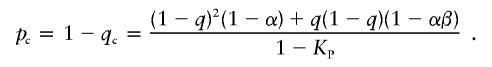
Similarly, for an unaffected control sample,

and equations for the classic recessive, classic dominant, additive, and multiplicative models are given in appendix B. Figure 2 shows the direction and magnitude of Δ_c for several dominant, recessive, additive, and multiplicative models.

Figure 2.

Δ_c plotted versus the susceptibility-allele frequency for controls. A, B, and D, Data points are as follows: γ=1.1 (blackened diamonds), γ=1.3 (unblackened triangles), γ=1.5 (blackened triangles), γ=2 (unblackened diamonds), γ=5 (blackened squares), and γ=10 (unblackened circles). A, Dominant model, K_P=0.1. B, Recessive model, K_P=0.2. C, Additive model, K_P=0.01. As in figure 1, because of our definition of an additive model (γ=2β and β>1), the data points in C are as follows: γ=4 (β=2) (unblackened diamonds), γ=2.2 (β=1.1) (blackened diamonds), γ=2.6 (β=1.3) (unblackened triangles), γ=3 (β=1.5) (blackened triangles), γ=2 (unblackened diamonds), γ=5 (blackened squares), and γ=10 (unblackened circles). D, Multiplicative model, K_P=0.05.

Number of Individuals Needed to Detect DHW

The χ² test of HWE for patients can be simplified to the following:

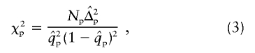where N_p is the number of patients and is the susceptibility-allele frequency estimated in patients (Weir 1996). A χ² value can also be determined for controls by using the susceptibility-allele frequency in controls (), Δ_c, and the number of controls in the sample (N_c). The power of the χ² test can be accounted for by using a noncentral χ² distribution with noncentrality parameter

(Weir 1996).

Given the above equations, it is straightforward to determine the number of individuals required to detect DHW for a specified level of significance and power, for patients and controls under any disease model. In figure 3, results for a variety of models are graphed in terms of N_p or N_c and the overall susceptibility-allele frequency for patients or controls. The results presented in figure 3A (patients) and 3B (controls) use a central χ² distribution corresponding to a significance level of 5% and 50% power, and the results presented in figure 3C (patients) and 3D (controls) use a noncentral χ² distribution corresponding to a significance level of 5% and 80% power.

Figure 3.

A, Number of patients needed to detect DHW as the susceptibility-allele frequency changes at a significance level of 5% and 50% power. Data points are as follows: dominant model with γ=1.3 (unblackened triangles), dominant model with γ=10 (unblackened circles), recessive model with γ=1.5 (blackened triangles), recessive model with γ=2 (unblackened diamonds), additive model with γ=2.2 (blackened diamonds), and additive model with γ=5 (blackened squares). B, Number of controls needed to detect DHW as the susceptibility-allele frequency changes at a significance level of 5% and 50% power. Data points are as follows: dominant model with K_P=0.2 and γ=10 (blackened circles), recessive model with K_P=0.05 and γ=10 (blackened circles), recessive model with K_P=0.2 and γ=5 (unblackened squares), additive model with K_P=0.2 and γ=5 (blackened squares), multiplicative model with K_P=0.1 and γ=10 (blackened squares with white cross), and multiplicative model with K_P=0.2 and γ=5 (blackened squares with white star). C, Same data points as A but assessed at 80% power. D, Same data points as B but assessed at 80% power.

For congruence with other studies reporting the results in terms of λ_s, the risk of disease in siblings of an affected individual relative to the risk in the general population, are summarized in appendix C with respect to common disease models. We also summarize results with respect to λ_s and Δ in figure 4.

Figure 4.

Sibling relative risk for dominant models with K_P=0.2 and varied γ values: γ=10 (unblackened circles), γ=5 (blackened squares), γ=2 (unblackened diamonds), and γ=1.5 (blackened triangles).

Goodness-of-Fit Test

Given the analytic framework characterized above and a set of observations in patients and controls with DHW in one or both samples, we proceed to identify the genetic disease model with the best fit to the genotypic proportions observed in patients and controls (constrained by the known lifetime prevalence of disease). If that “best-fit” model is, nevertheless, a poor fit to the observed data, as assessed by a χ² test with 1 df for a general model and 2 df for a restrictive (dominant, recessive, additive, or multiplicative) model (see appendix D), then it is unlikely that the underlying genetic disease model has generated the observed DHW; thus, alternative explanations for the DHW, including chance, genotyping error, and/or violations of the requisite assumptions of HWE, must be considered.

Examples

We chose several examples from the literature that illustrate how our results and software can help investigators distinguish a DHW consistent with genetic models from one that is not. The first example involves a DHW in patients but not in controls, with data derived from an association study of Crohn disease and a rare frameshift polymorphism (Leu3020fsinsC) in CARD15/NOD2 (Ogura et al. 2001; J. Cho, personal communication). The second example includes data from an association study that identified a highly significant association (P=3.3×10^-6) between LTA and myocardial infarction (MI) (Ozaki et al. 2002), attributable in part to the effect of significant DHW in both patients and controls in opposite directions. We also took advantage of several recent surveys of polymorphisms with DHW (Xu et al. 2002; Györffy et al. 2004; Kocsis et al. 2004a, 2004b; Osawa et al. 2004) to determine the proportion that are consistent with a genetic disease model (table 1).

Table 1.

Survey of DHW

			Genotype Distributionsb
PubMed ID	Diseasea	Gene	Patients	Controls	KP	q	α	β	γ	χ2	Pc
12221172	Alzheimer disease	A2M	61-48-23	98-77-9	.06	.264	.0513	1.085	2.966	1.016	NS
12105308	Alzheimer disease	APOE	4-18-94	6-53-74	.06	.758	.0269	1.000	3.137	1.013	NS
12105308	Alzheimer disease	APOE	31-49-29	67-102-19	.06	.381	.0449	1.251	2.509	4.221	.040
12105308	Alzheimer disease	APOE	57-118-100	58-97-48	.06	.482	.0462	1.118	2.027	.547	NS
12105308	Alzheimer disease	APOE	120-361-194	206-309-142	.06	.458	.0362	1.791	2.265	1.485	NS
11074789	Alzheimer disease	CST3	322-166-29	260-124-6	.05	.179	.0463	1.174	1.91	3.914	.048
11468325	Alzheimer disease	CST3	140-33-6	179-43-6	.06	.121	.059	1.000	2.114	4.064	NS
11468325	Alzheimer disease	CST3	137-34-8	180-40-8	.06	.13	.0587	1.000	2.343	9.671	.008
12034804	Alzheimer disease	IL-1β	5-40-39	15-107-95	.06	.679	.0365	1.718	1.718	4.812	NS
10869806	Alzheimer disease	IL-6 promoter	110-148-44	34-22-12	.05	.35	.043	1.257	1.377	5.111	.024
10815136	Alzheimer disease	PS1	3-45-45	3-24-18	.05	.66	.0141	3.803	3.94	1.929	NS
11124296	Macular degeneration	mEPHX	42-24-32	95-38-33	.01	.326	.00767	1.000	3.874	40.423	≪.001
10843185	Autoimmune hypothyrodism	IL-4	2-7-68	3-23-75	.02	.847	.00917	1.000	2.645	2.909	NS
10781645	Acute myocardial infarction	5-HT 2A receptor	39-133-83	43-150-62	.05	.538	.0362	1.435	1.568	8.829	.003
11781417	Blepharospasm	D1.1	25-51-15	42-32-16	.001	.361	.000673	1.804	1.875	4.485	.034
11142420	Breast cancer	CYP17	39-63-10	112-132-33	.05	.352	.0412	1.367	1.367	3.161	NS
10698474	Breast cancer	CYP1B1	37-101-48	44-127-29	.05	.468	.0357	1.504	1.678	15.736	7.3 × 10−5
10698474	Breast cancer	CYP1B1	26-68-27	26-78-17	.05	.464	.0379	1.446	1.446	11.11	.004
10698474	Breast cancer	CYP1B1	11-32-21	18-49-12	.05	.469	.0309	1.599	2.46	4.774	.029
11156391	Cancer toxicity (irinotecan)	UGT1A1	14-8-4	79-10-3	.01	.116	.00695	2.221	15.11	7.947	.005
12787424	Chronic allograft nephropathy	TGF-β1	0-22-8	23-83-67	.01	.613	0	11.76	11.76	4.204	NS
12787424	Chronic allograft nephropathy	TNFα	50-24-1	132-31-10	.01	.164	.00949	1.179	1.179	13.577	.001
10504487	Chronic renal failure	VDR	34-118-96	29-123-68	.005	.586	.00404	1.232	1.418	1.768	NS
10189842	Coeliac disease	CTLA-4	4-28-69	21-47-62	.01	.655	.00332	1.861	4.82	4.539	.033
10189842	Coeliac disease	CTLA-4	1-7-23	16-36-54	.01	.674	.003	1.731	5.43	5.198	.023
11889073	Colorectal cancer	MTHFR	28-35-12	204-229-34	.05	.324	.0415	1.231	1.995	7.478	.006
11889073	Colorectal cancer	MTHFR	28-64-94	114-560-533	.05	.669	.0455	1.000	1.223	10.133	.006
11889073	Colorectal cancer	MTHFR	14-66-73	39-116-148	.05	.678	.0431	1.161	1.195	4.313	.038
10794488	Colorectal polyps	MTHFR	98-72-26	297-258-71	.05	.315	.0484	1.000	1.338	4.323	NS
12631667	Crohn disease	CYP1A1	2-20-129	5-22-122	.05	.879	.0325	1.000	1.698	7.497	.024
12631667	Crohn disease	EPXH	20-60-71	59-58-32	.05	.428	.0201	2.046	6.307	6.759	.009
12631669	Crohn disease	NOD2	248-20-3	290-10-0	.05	.0206	.0478	1.929	20.71	.454	NS
11402126	Dementia	ACE	74-239-120	98-233-144	.1	.539	.0808	1.301	1.301	2.457	NS
12221164	Epilepsy	OPRM1	193-29-8	208-20-0	.01	.0451	.0092	1.592	18.719	.399	NS
9607207	Hypertension/nephroangiosclerosis	ACE	6-10-21	8-48-19	.05	.557	.0312	1.000	2.933	7.18	.028
10792336	IDDM	VDR	137-16-4	231-16-1	.05	.046	.0482	1.236	9.315	3.482	NS
11231353	IDDM nephropathy	GLUT1	3-29-10	21-60-23	.005	.495	.00139	4.482	4.482	3.604	NS
11097227	Lung cancer	HRAS1	17-86-209	21-134-276	.01	.789	.00882	1.000	1.214	3.239	NS
11097227	Lung cancer	HRAS1	8-19-49	8-38-54	.01	.71	.00742	1.000	1.692	3.583	NS
11097227	Lung cancer	TP53	9-16-26	57-192-197	.01	.652	.00883	1.000	1.311	4.33	NS
11045785	Lung cancer, squamous cell	p53	16-44-73	61-212-237	.01	.668	.00823	1.000	1.48	3.481	NS
9844142	Macroangiopathy	PAI-1	6-28-22	22-88-42	.05	.567	.0295	1.683	2.116	4.958	.026
11122322	Myocardial infarction	ACE	184-460-217	193-393-215	.1	.508	.0884	1.174	1.174	1.748	NS
10712418	Myocardial infarction	TF-1208	227-361-218	197-349-186	.1	.483	.0956	1.000	1.199	6.502	.039
10680782	Multiple sclerosis	GSTM3	276-97-14	221-64-15	.05	.161	.0496	1.000	1.336	11.722	.003
15338456d	NIDDM	RETN	48-85-16	63-83-12	.054	.336	.0396	1.649	1.649	6.384	.041
10231446	NIDDM nephropathy	GLUT1	43-78-10	77-41-6	.05	.219	.0269	3.199	3.199	.0884	NS
10231446	NIDDM nephropathy	GLUT1	12-48-4	77-41-6	.05	.219	.0153	6.818	6.818	1.099	NS
9844142	NIDDM nephropathy	PAI-1	64-116-28	66-80-31	.05	.388	.0409	1.357	1.357	2.616	NS
9844142	NIDDM nephropathy	PAI-1	28-58-12	66-80-31	.05	.392	.0383	1.484	1.484	2.745	NS
12675860	NIDDM nephropathy	TGF-β1	24-24-17	27-26-5	.3	.354	.258	1.000	2.29	.537	NS
10964048	Oral cancer	CYP1A1	96-36-13	104-54-6	.01	.186	.00943	1.000	2.732	1.638	NS
10964048	Oral cancer	CYP1A1	56-55-31	62-65-15	.01	.332	.0087	1.02	2.275	.0473	NS
11914402	Parkinson disease	Nurr1	162-48-15	174-45-2	.02	.112	.0183	1.172	5.822	.14	NS
11786085	Renal parenchymal scarring	TGF-β1	0-27-16	16-76-79	.01	.669	.001	11.11	11.11	3.973	NS
11786085	Renal parenchymal scarring	TGF-β1	13-27-3	73-72-26	.01	.303	.00551	4.001	3.95	.0627	NS
10430441	Stroke	NOS3	109-125-31	154-203-36	.15	.353	.15	1.000	1.004	7.466	.024
11027931	Venous thrombosis	β-fibrogen	2-6-82	0-22-163	.01	.926	.00892	1.000	1.141	9.55	.008
11027931	Venous thrombosis	Factor 7	67-19-5	148-33-4	.01	.115	.0094	1.096	4.351	1.758	NS
12753258	Vertebral fracture	COLIA1	10-2-5	75-35-6	.01	.2	.00754	1	9.125	2.24	NS

^aIDDM = insulin-dependent diabetes mellitus; NIDDM = non–insulin-dependent diabetes mellitus.

^bIn the genotype distributions for patients and controls, the three numbers separated by hyphens represent the nonsusceptible homozygotes, the heterozygotes, and the susceptible homozygotes.

^cNS = not significant.

^dOsawa et al. (2004)

Results

Magnitude of Δ

As noted elsewhere, the larger the value of Δ, the more the genotypic frequency departs from HWE expectations (Weir 1996). In patients, the magnitude of Δ_p is determined by q, γ, and β, as shown in equation (1) above. The maximum value for Δ_p, given a genetic disease model, occurs at the susceptibility-allele frequency that maximizes the HWE-expected proportion of heterozygotes affected with disease (g_Aa) and can be calculated by

For example, the maximum Δ_p for a dominant model with γ=1.5 occurs when the allele frequency is 0.45, which corresponds to the highest proportion of HWE-expected heterozygotes among patients (g_Aa=0.5505) under this model.

In controls, Δ_c is a function of K_P, α, β, γ, and q. Larger Δ_c values occur as the prevalence of disease in the general population increases, whereas, in patients, K_P has no direct effect on the size of Δ_p. For example, a dominant model with γ=1.5 and q=0.33 leads to a Δ_c of 0.00209 when K_P=0.1 and a Δ_c of 0.000193 when K_P=0.01. Larger Δ_c values also occur with higher γ values, as shown in figure 2. The susceptibility-allele frequency also affects the magnitude of Δ_c, with common allele frequencies (0.1⩽q⩽0.8) corresponding to larger Δ_c values and with allele frequencies at the tails of the frequency spectrum corresponding to smaller Δ_c values.

Direction of Δ

The direction of Δ is vital to understanding whether an observed DHW can be due to the underlying genetic model, and, for patients, the disease model specifies the direction of Δ_p (table 2). The additive model is different than the dominant, recessive, or multiplicative models, in that Δ_p can be positive, negative, or zero. Δ_p is positive when 2 < γ < 4 and negative when γ>4. However, when γ=4, the additive model is equivalent to the multiplicative model (β=2 and γ=4), and Δ_p is equal to 0 (i.e., no DHW is expected). The general model is dependent on the value associated with β, where Δ_p is positive if γ>β² and negative if γ<β².

Table 2.

Direction of DHW, Given a Genetic Disease Model and Parameter Values^[Note]

	Direction of DHW in
Model	Patients	Controls
Dominant	−	+
Recessive	+	−
Additive	If γ<2, +;if γ>2, −;if γ=2, 0	−
Multiplicative	0	−
General	If γ>β2, +;if γ<β2, −	If γ+1+αβ2>2β+αγ, −; if γ+1+αβ2<2β+αγ, +

Note.— A plus sign (+) represents an excess of homozygotes, and a minus sign (−) represents a deficiency of homozogyotes.

The direction of Δ in controls is also dependent on the underlying genetic disease model, and, for dominant and recessive models, Δ_c is in the direction opposite that observed in patients. Interestingly, Δ_c for controls under the additive model does not change with γ, as observed for patients, but always shows an excess of heterozygotes (Δ_c<0). However, there is an asymmetry in the homozygote classes when Δ≠0 for both patients and controls, with patients showing an excess of disease-susceptible homozygotes and controls showing an excess of wild-type homozygotes. The multiplicative model generates Δ values for controls similar to those generated by the recessive and additive models, with Δ_c<0. The direction of DHW for a general disease model in controls is negative if γ+1+αβ²>2β+αγ and positive if the inequality is reversed (i.e., γ+1+αβ²<2β+αγ).

Number of Individuals Needed to Detect DHW for a Specified Significance and Power

As might be expected, fewer patients are needed to detect DHW as the genotype relative risk increases. It is notable, however, that low γ values (e.g., 1.5) can produce DHW with relatively small samples of patients. For example, <500 patients are needed to detect DHW (at a significance level of 5% and 50% power) under a recessive model with γ=1.5 and over a range of susceptibility-allele frequencies from 0.29 to 0.63. As γ increases to 2, the range of susceptibility-allele frequencies increases to 0.11–0.81, with a minimum sample size of ∼130 patients when q=0.4 with 50% power (fig. 3A) and 267 patients with 80% power (fig. 3C). An additive model, however, requires a minimum of ∼750 patients at q=0.38 to detect DHW with γ=3, but the required sample size decreases to 176 patients with γ=2.2. As shown above, Δ_p increases for additive models as γ increases or decreases from 4. Therefore, at a significance level of 5% and 50% power, an additive model can lead to detection of DHW in 176 patients when either γ=2.2 or γ=7.56. The difference between the two observations, however, is the direction of the DHW, in which the former (γ=2.2) shows an excess of homozygotes and the latter (γ=7.56) shows a deficiency of homozygotes.

The number of controls needed to detect DHW is generally much larger but is often still within the range of commonly collected sample sizes for a wide range of models. As with patients, the number of controls required to detect DHW decreases as γ increases. But, unlike in the calculations for patients, K_P also determines the number of controls needed to detect DHW. For dominant models, <1,000 unaffected individuals are needed to detect DHW when K_P=0.2 and γ⩾5 with 50% power (fig. 3B), and <2,000 controls with 80% power (fig. 3D). Because of the specifications of the additive model, the same effect is observed in controls as in patients, whereby a decrease in the number of controls needed to detect DHW occurs as γ increases or decreases from 4. Recessive models with γ⩾5 can lead to detection of DHW in <200 controls with 50% power when K_P=0.2. When K_P decreases to as low as 0.05, ∼1,000 controls are needed to detect DHW for the recessive model with γ⩾10 and q=0.23 (fig. 3B). Multiplicative models show DHW in a sample of <2,000 controls when K_P⩾0.1 and γ⩾10 and in a sample of <1,200 controls when K_P⩾0.2 and γ⩾5 (at 50% power and a significance level of 5%). Generally, larger Δ_c values are associated with models specified by high K_P values (e.g., K_P⩾0.2) and high γ values (e.g., γ⩾5).

Sibling Relative Risk Values that Correspond to Expected DHW

We calculated λ_s for all models studied, to understand the results for these common disease models relative to those of previous studies that assessed power by using this parameter. As expected, λ_s increases as K_P decreases, and, overall, the resulting λ_s values (including those that are expected to give DHW in a small sample) are quite small. For dominant models or recessive models (γ=1.5), in which DHW is expected for samples of <500 patients, λ_s is <1.03 (fig. 4). For additive models, in which <1,400 patients are needed to detect DHW, λ_s values do not exceed 1.18. Thus, DHW can be observed for strikingly low λ_s values in sample sizes currently being used for large-scale association studies.

Example 1: DHW in Patients Only

Ogura et al. (2001) conducted a case-control association study of Crohn disease to fine map IBD1 in the pericentromeric region of chromosome 16. They identified a cytosine insertion (Leu3020fsinsC) in CARD15/NOD2 that causes a truncated NOD2 protein and that results in deficient activation of NF-κB and the immune response. We calculated HWE for the Leu3020fsinsC (Cins) polymorphism in unrelated Jewish and European American patients with Crohn disease and in unrelated controls. Because of the low proportion of HWE-expected homozygotes, we used Fisher’s exact test to determine DHW (Weir 1996). The distribution of genotypes in Jewish patients was 121 wild-type (wt)/wt homozygotes, 15 Cins/wt heterozygotes, and 4 Cins/Cins homozygotes, which yields P=.0059. The genotype distribution in European American patients was 314 wt/wt homozygotes, 41 Cins/wt heterozygotes, and 9 Cins/Cins homozygotes. Fisher’s exact test generates P=1.28×10^-4, which is also highly significant. When all unrelated patients are tested for DHW (456 wt/wt homozygotes, 61 Cins/wt heterozygotes, and 13 Cins/Cins homozygotes), P=6.83×10^-6. All three populations of patients showed significant DHW, with an excess of homozygotes. The distribution of genotypes in all controls was 311 wt/wt homozygotes, 25 Cins/wt heterozygotes, and 0 Cins/Cins homozygotes, which is consistent with HWE.

If the allele frequencies in both the patients (q_p=0.082) and the controls (q_c=0.037) are used to help delineate the general genetic disease model that best fits the observed genotypic distributions, we find that it can be characterized by K_P=0.002, q=0.0379, α=0.00186, β=1.696, and γ=18.338. If a χ² test is performed to determine the goodness-of-fit of the expected number of patients and controls, given the model that best fits the observed genotypic counts, χ²=0.478 (P=.827 with 1 df); thus, the best-fit model is a good fit to the observed data. Moreover, the model is consistent with what has been obtained elsewhere for other types of data (Hampe et al. 2001; Ogura et al. 2001).

Example 2: DHW in Opposite Directions in Patients and Controls

Ozaki et al. (2002) published a large-scale association study designed to identify genetic variation affecting risk of MI in a Japanese sample. The study involved an initial screen of >92,000 SNPs in a small sample and follow-up studies for those SNPs with evidence of association (P<.01 for a dominant or recessive model) performed in a larger sample (1,133 patients, 1,006 random controls, and 872 age-matched random controls). This led to more intensive studies of the LTA region (near HLA on 6p21), with 5 of 26 SNPs genotyped in the region showing highly significant association with MI (e.g., for LTA exon 1 polymorphism, P=3.3×10^-6).

Although Ozaki et al. (2002) reported that all 26 SNPs were in HWE, with P>.01, we note that each of the 5 SNPs for which genotype distributions are published show a significant DHW in opposite directions for patients and controls. The LTA exon 1 polymorphism is the most significantly associated with MI, with a genotype distribution among the 1,133 patients of 416 GG homozygotes, 504 GA heterozygtoes, and 213 AA homozygotes, which yields χ²=7.40 (P=.0065)—an excess of homozygotes relative to HWE-expected genotype proportions. The genotype distribution among the 1,006 random controls is 378 GG homozygotes, 512 GA heterozygotes, and 116 AA homozygotes. This sample of controls generates χ²=8.51 (P=.0035) but shows a deviation in the opposite direction of patients, with a deficiency of homozygotes. The age-matched random control group of 872 individuals has a genotype distribution of 344 GG homozygotes, 428 GA heterozygotes, and 100 AA homozygotes, corresponding to a nonsignificant χ²=3.69 (P=.055) but also showing a deficiency of homozygotes similar to that seen for the 1,006 random controls.

The first problem easily identified is that a significant DHW is observed in a sample that may be better characterized as a random sample than a control sample and thus would not be expected to show DHW, regardless of the underlying genetic disease model. If we assume that the control sample is a control sample, rather than a random sample, the best-fit model is K_P=0.01, q=0.371, α=0.00932, β=1.024, and γ=1.469. The goodness-of-fit to the observed data is significantly poor, with χ²=5.024 (P=.025 with 1 df). Given that the best-fit model is not a good fit to what is observed in the 1,133 patients and 1,006 controls, the underlying genetic disease model for a susceptibility locus in that region is therefore an unlikely explanation for the observed DHW.

Survey of DHW

We identified 41 association studies with 60 polymorphisms that depart from HWE, from several recent reviews (Xu et al. 2002; Györffy et al. 2004; Kocsis et al. 2004a, 2004b; Osawa et al. 2004) (table 1). All K_P values were either given by the association study or were identified on the World Health Organization Web site. There are 35 polymorphisms that depart from HWE in patients only, 21 that depart in controls only, 2 that depart in the same direction in patients and controls, and 1 that departs in the opposite direction in patients and controls. Of those that have a dominant or recessive model as the best-fit genetic model, 35.3% (12 of 34) did not have a genetic model that fit the observed genotype distributions. Of those for which the best-fit model was a general model, 53.8% (14 of 26) did not have a model that fit well the observed data. Therefore, 43.3% of the polymorphisms we identified from the reviews are inconsistent with a biological reason for the observed DHW. This highlights the importance not only of correctly assessing HWE for genotype data but also of understanding whether an observed DHW is consistent with a genetic model of disease susceptibility.

Discussion

Investigators have taken surprisingly inconsistent pathways in the interpretation and use of DHW. In some cases, investigators report significant association between variation at candidate genes and complex disorders that is quite dependent on the existence of DHW (i.e., the associations are genotypic rather than allelic, and the genotypic differences are driven by DHW). In at least some situations, the observed DHW is implausible from a biological perspective, which calls into question the association result. On the other hand, some investigators believe that any marker showing a DHW is likely to be erroneous and/or misleading; as a result, they may be throwing away information valuable for mapping and identifying causal polymorphisms. With the analytic framework and software we have developed, we provide a way for investigators to assess markers with DHW in a more logical and systematic way by distinguishing those that could be attributed to the underlying genetic model at the susceptibility locus from those due to genotyping errors, chance, and/or violations of the assumptions of HWE, thereby improving the quality of scientific inferences.

Given the increasing sample sizes contemplated for large-scale association studies, it would seem that DHW is a neglected and potentially fruitful avenue for further research to improve signal localization. Results of studies of the CARD15/NOD2 region provide support for this notion. A common coding polymorphism (P268S) (q=0.35 in patients with Crohn disease, and q=0.29 in unaffected controls) shows significant DHW, with an excess of homozygotes in both Jewish patients (P=.0277) and in patients overall (P=.00546) (J. Cho, personal communication). The best-fit model for this polymorphism provides a good fit to the observed genotypic distributions (χ²=1.501×10^-10; P=1.0 with 1 df). Although this polymorphism is not thought to affect the risk of Crohn disease, three of the known susceptibility alleles (Leu3020fsinsC, Gly908Arg, and Arg702Trp) are in the same haplotype as the more rare allele at this site. If patients with any of those mutations are removed from the patient population and HWE is reassessed, the DHW is no longer significant (P=.2115 for Jewish patients, and P=.632 for patients overall). If none of the causative SNPs had been previously identified, the observation that the common polymorphism departed from HWE in a way that was consistent with a genetic model could have been used to support further investigation of the local region. This observation highlights the value of using DHW when fine mapping complex diseases, as originally hypothesized by Nielsen et al. (1998).

Given the relatively large sample sizes used in modern candidate-gene studies as well as in fine-mapping and positional cloning studies, and the fact that DHW should be expected for a wide range of genetic disease models (consistent with the modest genetic contributions likely to be relevant for complex disorders), it is perhaps surprising that we have not seen a larger number of markers reported to show DHW. Of 60 SNPs from association studies in which DHW has been identified in patients and/or controls and in which both patient and control genotype distributions are available, 34 (56.7%) have genotype distributions consistent with the expectations from a best-fit model (table 1). DHW in patients is never expected for a multiplicative model and is less likely to be detected as significant for a model with susceptibility-allele frequencies at the tails of the frequency spectrum. We have not examined the consequences for HWE in more-complex disease models with allelic or locus epistasis, profound sex effects, etc., and, if such models were standard for complex disorders, it is unclear what the consequences would be. Thus, the failure to more often observe DHW at polymorphisms hypothesized to affect susceptibility to complex disorders may reflect biological characteristics of the genetic disease model that make such DHW impossible or at least less likely.

It is also possible that investigators mistrust data with DHW and may sometimes ignore such polymorphisms with DHW in their studies. Systematic errors in genotyping or nonrandom patterns of missing data may generate a relatively consistent pattern of DHW (e.g., disproportionate missing data in heterozygotes may lead to a consistent pattern of DHW, with an excess of homozygotes). Other types of error may be more sporadic. An unrecognized polymorphism in primer sequences used in subsequent PCR may lead to DHW, with an excess of homozygotes, particularly when the primer polymorphism is in LD with one of the test alleles. Genomic duplications or deletions can also lead to DHW. Because even the systematic errors will not be universal, error and nonrandom patterns of missing data may be detectable in a single marker within a set that are in strong LD. In contrast, when markers have DHW due to violations of assumptions of HWE or to chance, markers in LD may show similar patterns of DHW. Independent samples will tend not to replicate chance DHW but may replicate DHW due to violations of HWE assumptions. Clearly, genomewide or large-scale studies offer additional information for interpretation of DHW, including, for example, the ability to examine potential population substructure. Many of the studies summarized in table 1, however, focus on one or a small number of candidate genes, and the approaches we propose offer a unique opportunity to improve the scientific inferences about observed DHW. It should also be noted that just because an observed DHW is consistent with genetic models does not mean that errors, missing data patterns, or violations of HWE assumptions did not generate or contribute to the observed DHW, and DHW can no doubt be attributable to a combination of factors. Finally, it should also be noted that investigators frequently underestimate the significance of observed DHW, probably because of a misunderstanding of the degrees of freedom associated with the test.

Appendix A: Δ in Patients

Weir (1996) defines Δ as the difference between the population and HWE-expected genotypic frequencies. Therefore, we first define these genotypic frequencies in terms of q, the susceptibility-allele frequency in the general population; α, the baseline penetrance for wild-type homozgyotes; β, the relative risk to heterozygotes; γ, the relative risk to homozygotes for the susceptibility allele; and K_P, the population prevalence of disease. The expected genotypic proportions in patients, under the assumption of HWE in the general population, are as follows:

The expected susceptibility-allele frequency for patients is

The frequency of the wild-type allele in patients is

Therefore,

which then simplifies to equation (1).

For a classic recessive model, where β=1 and γ>1,

For a classic dominant model, where β=γ and γ>1,

For an additive model, where γ=2β and β>1,

As explained in the “Methods” section, the multiplicative model for patients, where β²=γ and β>1, simplifies to Δ_p=0.

Appendix B: Δ in Controls

As defined for patients in appendix A, we define the genotypic proportions in controls for a general disease model as

The expected susceptibility-allele frequency in controls is

The frequency of the wild-type allele in controls is

Therefore,

which simplifies to equation (2).

For a classic recessive model, where β=1 and γ>1,

For a classic dominant model, where β=γ and γ>1,

For an additive model, where γ=2β and β>1,

Finally, for a multiplicative model, where γ=β² and β>1,

Appendix C: λ_s Values

Given that

(Risch 1990), where V_A is the additive variance that can be calculated by

and V_D is the dominance variance that can be calculated by

λ_s under the classic dominant model can then be calculated as

λ_s under the classic recessive model can be calculated as

λ_s under the additive model can be calculated as

and, finally, λ_s under the multiplicative model can be calculated as

Appendix D: Goodness-of-Fit Test

The expected genotypic proportions for patients under a genetic disease model are g_AA-p, g_Aa−p, and g_aa-p, as found in appendix A. The expected genotypic proportions for controls under a genetic disease model are g_AA-c, g_Aa-c, and g_aa-c, as found in appendix B.

For a particular set of disease model parameter values (α, β, γ, and q), where the total number of patients is N_p, the total number of controls denoted is N_c, and the observed number of patients (or controls), given a specific genotype, is N_genotype-p (or N_genotype-c), the goodness-of-fit test is as follows:

Minimizing the resulting test statistic over the entire parameter space, subject to appropriate constraints on α, β, γ, and q and where K_P is fixed, yields parameter estimates that are approximately maximum-likelihood estimates. The minimal value of the test statistic is approximately distributed as a χ² with 1 df for a general model and 2 df for restricted models (i.e., dominant, recessive, additive, and multiplicative models) (Cramer 1946). We verify through simulations that applying this test to data showing a DHW does not affect the resulting distribution of the test statistic. We generated 1,000 replicates of 1,000 patients and 1,000 controls under a dominant, recessive, or general disease model as specified by the penetrances, which offer an advantage in being bound between 0 and 1. We kept for further analysis only replicates that showed DHW in patients, in controls, or in both patients and controls. We used the goodness-of-fit test to find the best-fit genetic model for each simulation and compared the resulting χ² value to 1,000 simulated χ² values, given the specified degrees of freedom (fig. 5).

Figure 5.

Simulations with the goodness-of-fit test. A, 1,000 simulations of a disease locus constructed under a general model (q=0.20, α=0.12, β=2.67, and γ=4.33), a dominant model (q=0.20, α=0.11, and β=γ=3.27), and a recessive model (q=0.20, α=β=0.18, and γ=3.78), in which the population prevalence is high (K_P=0.20). Each simulation, in which DHW was observed in patients and/or controls, was assessed using the goodness-of-fit test and was compared with a simulated distribution of 1,000 χ² values, with 1 df for a general model and 2 df for a dominant or recessive model. B, 1,000 simulations of a disease locus at a lower population prevalence (K_P=0.005) than A constructed under a general model (q=0.10, α=0.003, β=4.17, and γ=10.67), a dominant model (q=0.10, α=0.0027, and β=γ=5.48), and a recessive model (q=0.10, α=β=0.0048, and γ=5.17).

If the goodness-of-fit test, with 1 df for a general model or 2 df for a restrictive model, corresponds to a P value less than the specified threshold, the genetic disease model can be rejected as a poor fit to the observed data. Note that rare-allele frequencies, which may produce low genotype counts, may produce approximations from the goodness-of-fit test that do not perform as expected.

References

- Castle WE (1903) The laws of heredity of Galton and Mendel, and some laws governing race improvement by selection. Proc Am Acad Arts Sci 39:223–242 [Google Scholar]
- Cramer H (1946) Mathematical methods of statistics. Princeton University Press, Princeton, NJ [Google Scholar]
- Gomes I, Collins A, Lonjou C, Thomas NS, Wilkinson J, Watson M, Morton N (1999) Hardy-Weinberg quality control. Ann Hum Genet 63:535–538 10.1046/j.1469-1809.1999.6360535.x [DOI] [PubMed] [Google Scholar]
- Györffy B, Kocsis I, Vásárhelyi B (2004) Biallelic genotype distributions in papers published in Gut between 1998 and 2003: altered conclusions after recalculating the Hardy-Weinberg equilibrium. Gut 53:614–616 [DOI] [PMC free article] [PubMed] [Google Scholar]
- Hampe J, Cuthbert A, Croucher PJP, Mirza MM, Mascheretti S, Fischer S, Frenzel H, King K, Hasselmeyer A, MacPherson AJS, Bridger S, van Deventer S, Forbes A, Nikolaus S, Lennard-Jones JE, Foelsch UR, Krawczak M, Lewis C, Schreiber S, Mathew CG (2001) Association between insertion mutation in NOD2 gene and Crohn’s disease in German and British populations. Lancet 357:1925–1928 10.1016/S0140-6736(00)05063-7 [DOI] [PubMed] [Google Scholar]
- Hardy GH (1908) Mendelian proportions in a mixed population. Science 18:49–50 [DOI] [PubMed] [Google Scholar]
- Hosking L, Lumsden S, Lewis K, Yeo A, McCarthy L, Bansal A, Riley J, Purvis I, Xu CF (2004) Detection of genotyping errors by Hardy-Weinberg equilibrium testing. Eur J Hum Genet 12:395–399 10.1038/sj.ejhg.5201164 [DOI] [PubMed] [Google Scholar]
- Kocsis I, Györffy B, Németh E, Vásárhelyi B (2004a) Examination of Hardy-Weinberg equilibrium in papers of Kidney International: an underused tool. Kidney Int 65:1956–1958 10.1111/j.1523-1755.2004.00596.x [DOI] [PubMed] [Google Scholar]
- Kocsis I, Vásárhelyi B, Györffy A, Györffy B (2004b) Reanalysis of genotype distributions published in Neurology between 1999 and 2002. Neurology 63:357–358 [DOI] [PubMed] [Google Scholar]
- Levecque C, Elbaz A, Clavel J, Richard F, Vidal J, Amouyel P, Tzourio C, Alpérovitch A, Chartier-Harlin M (2003) Association between Parkinson’s disease and polymorphisms in the nNos and iNos genes in a community-based case-control study. Hum Mol Genet 12:79–86 10.1093/hmg/ddg009 [DOI] [PubMed] [Google Scholar]
- Li CC (1967) Castle’s early work on selection and equilibrium. Am J Hum Genet 19:70–74 [PMC free article] [PubMed] [Google Scholar]
- Martin ER, Lai EH, Gilbert JR, Rogala AR, Afshari AJ, Riley J, Finch KL, Stevens JF, Livak KJ, Slotterbeck BD, Slifer SH, Warren LL, Conneally PM, Schmechel DE, Purvis I, Pericak-Vance MA, Roses AD, Vance JM (2000) SNPing away at complex diseases: analysis of single-nucleotide polymorphisms around APOE in Alzheimer disease. Am J Hum Genet 67:383–394 [DOI] [PMC free article] [PubMed] [Google Scholar]
- Nejentsev S, Laaksonen M, Tienari PJ, Fernandez O, Cordell H, Ruutiainen J, Wikström J, Pastinen T, Kuokkanen S, Hillert J, Ilonen J (2003) Intercellular adhesion molecule-1 K469E polymorphism: study of association with multiple sclerosis. Hum Immunol 64:345–349 10.1016/S0198-8859(02)00825-X [DOI] [PubMed] [Google Scholar]
- Nielsen DM, Ehm MG, Weir BS (1998) Detecting marker-disease association by testing for Hardy-Weinberg disequilibrium at a marker locus. Am J Hum Genet 63:1531–1540 [DOI] [PMC free article] [PubMed] [Google Scholar]
- Ogura Y, Bonen DK, Inohara N, Nicolae DL, Chen FF, Ramos R, Britton H, Moran T, Karaliuskas R, Duerr RH, Achkar J-P, Brant SR, Bayless TM, Kirschner BS, Hanauer SB, Nuñez G, Cho JH (2001) A frameshift mutation in NOD2 associated with susceptibility to Crohn’s disease. Nature 411:603–606 10.1038/35079114 [DOI] [PubMed] [Google Scholar]
- Oka A, Tamiya G, Tomizawa M, Ota M, Katsuyama Y, Makino S, Shiina T, Yoshitome M, Iizuka M, Sasao Y, Iwashita K, Kawakubo Y, Sugai J, Ozawa A, Ohkido M, Kimura M, Bahram S, Inoko H (1999) Association analysis using refined microsatellite markers localizes a susceptibility locus for psoriasis vulgaris within a 111 kb segment telomeric to the HLA-C gene. Hum Mol Genet 8:2165–2170 10.1093/hmg/8.12.2165 [DOI] [PubMed] [Google Scholar]
- Osawa H, Yamada K, Onuma H, Murakami A, Ochi M, Kawata H, Nishimiya T, Niiya T, Shimizu I, Nishida W, Hashiramoto M, Kanatsuka A, Fujii Y, Ohashi J, Makino H (2004) The G/G genotype of a resistin single-nucleotide polymorphism at −420 increases type 2 diabetes mellitus susceptibility by inducing promoter activity through specific binding of Sp1/3. Am J Hum Genet 75:678–686 [DOI] [PMC free article] [PubMed] [Google Scholar]
- Ozaki K, Ohnishi Y, Iida A, Sekine A, Yamada R, Tsunoda T, Sato H, Sato H, Hori M, Nakamura Y, Tanaka T (2002) Function SNPs in the lymphotoxin-α gene that are associated with susceptibility to myocardial infarction. Nat Genet 32:650–654 10.1038/ng1047 [DOI] [PubMed] [Google Scholar]
- Risch N (1990) Linkage strategies for genetically complex traits. I. Multilocus models. Am J Hum Genet 46:222–228 [PMC free article] [PubMed] [Google Scholar]
- Wang L, Sato K, Tsuchiya N, Yu J, Ohyama C, Satoh S, Habuchi T, Ogawa O, Kato T (2003) Polymorphisms in prostate-specific antigen (PSA) gene, risk of prostate cancer, and serum PSA levels in Japanese population. Cancer Letters 202:53–59 10.1016/j.canlet.2003.08.001 [DOI] [PubMed] [Google Scholar]
- Weinberg W (1908) On the demonstration of heredity in man. In: Boyer SH (ed) (1963) Papers on human genetics. Prentice-Hall, Englewood Cliffs, NJ [Google Scholar]
- Weir BS (1996) Disequilibrium. In: Genetic data analysis II: methods for discrete population genetic data. Sinaur Associates, Sunderland, MA, pp 91–139 [Google Scholar]
- Xu J, Turner A, Little J, Bleecker ER, Meyers DA (2002) Positive results in association studies are associated with departure from Hardy-Weinberg equilibrium: hint for genotyping error? Hum Genet 111:573–574 10.1007/s00439-002-0819-y [DOI] [PubMed] [Google Scholar]
- Xu J, Zheng SL, Hawkins GA, Faith DA, Kelly B, Isaacs SD, Wiley KE, Chang B, Ewing CM, Bujnovszky P, Carpten JD, Bleecker ER, Walsh PC, Trent JM, Meyers DA, Isaacs WB (2001) Linkage and association studies of prostate cancer susceptibility: evidence for linkage at 8p22-23. Am J Hum Genet 69:341–350 [DOI] [PMC free article] [PubMed] [Google Scholar]