

Abstract
Background
Manual contour corrections during fractionated magnetic resonance (MR)‐guided radiotherapy (MRgRT) are time‐consuming. Conventional population models for deep learning auto‐segmentation might be suboptimal for MRgRT at MR‐Linacs since they do not incorporate manual segmentation from treatment planning and previous fractions.
Purpose
In this work, we investigate patient‐specific (PS) auto‐segmentation methods leveraging expert‐segmented planning and prior fraction MR images (MRIs) to improve auto‐segmentation on consecutive treatment days.
Materials and Methods
Data from 151 abdominal cancer patients treated at a 0.35 T MR‐Linac (151 planning and 215 fraction MRIs) were included. Population baseline models (BMs) were trained on 107 planning MRIs for one‐class segmentation of the aorta, bowel, duodenum, kidneys, liver, spinal canal, and stomach. PS models were obtained by fine‐tuning the BMs using the planning MRI (). Maximal improvement by continuously updating the PS models was investigated by adding the first four out of five fraction MRIs (). Similarly, PS models without BM were trained ( and ). All hyperparameters were optimized using 23 patients, and the methods were tested on the remaining 21 patients. Evaluation involved Dice similarity coefficient (DSC), average () and the 95th percentile (HD95) Hausdorff distance. A qualitative contour assessment by a radiation oncologist was performed for BM, , and .
Results
and networks had the best geometric performance. and BMs showed similar DSC and HDs values, however models outperformed BMs. predictions scored the best in the qualitative evaluation, followed by the BMs and models.
Conclusion
Personalized auto‐segmentation models outperformed the population BMs. In most cases, delineations were judged to be directly usable for treatment adaptation without further corrections, suggesting a potential time saving during fractionated treatment.
Keywords: auto‐segmentation, MR‐Linac, patient‐specific transfer learning
1. INTRODUCTION
Magnetic resonance linear accelerators (MR‐Linacs) enable online adaptive MR‐guided radiation therapy (MRgRT). 1 , 2 This technology allows for the monitoring of anatomical changes prior to and during patient irradiation, with no additional imaging dose. As a consequence, the ablative dose can be delivered in fewer fractions and with reduced safety margins. 3 , 4 , 5
The currently available commercial solution for deep learning (DL) auto‐segmentation at MR‐Linacs 6 and the majority of published research 7 , 8 , 9 , 10 employ population‐based DL models trained on larger datasets of expert‐segmented MR images (MRIs). By design, the networks learn common features shared among a wide range of patients, thus generating segmentations that are combinations of the examples they were trained on. However, this may be a sub‐optimal solution for fractionated treatment, that consists of a pre‐treatment planning phase and the subsequent series of irradiations called fractions. 11 During irradiation, the manually segmented planning MRI, as well as images from previous fractions with contours approved by radiation oncologists, are available but not integrated into the population models.
Previous studies have examined whether utilizing a patient's segmented planning MRI for fine‐tuning a population model 12 , 13 or training from scratch 14 can enhance the auto‐segmentation performance of fraction images in prostate patients. A similar 2D method for patients diagnosed with cancer in the abdomen region was presented by Li et al., 15 where the personalized models were updated daily with newly acquired data. Nevertheless, each of the presented studies exclusively focused on a single method, and all of them come with their limitations. The first two were conducted for prostate cases, where patient anatomy is relatively simple and stable. The last one included only six patients, permitting only a limited evaluation of the presented methods.
The goal of this work was to perform an investigation of approaches leveraging prior knowledge available in MRgRT in order to enhance the quality of abdominal organs‐at‐risk (OARs) auto‐segmentation on fraction MRIs. Four methods of generating patient‐specific (PS) models were compared to population baseline models (BMs) via geometric metrics and a qualitative evaluation by a trained radiation oncologist. The BMs were fine‐tuned using either only the segmented planning image or the planning and first four out of five fraction images of a specific patient. Furthermore, personalized models were trained from scratch instead of using BMs as a starting point, with only the planning or the planning and first four fraction MRIs. To the best of our knowledge, this is the first study to investigate the impact of population BMs on personalized segmentation models, combining them with progressive training and comparing these methods with approaches relying solely on individual patient data.
2. MATERIAL AND METHODS
2.1. Dataset and data pre‐processing
The dataset was collected retrospectively and comprised 151 cases, including 84 males and 67 females. The median of patient's age was 68 years, ranging from 34 to 91 years old. These patients were treated at the 0.35 T MR‐Linac (MRIdian, ViewRay Inc, Cleveland, Ohio) at the Department of Radiation Oncology of the LMU Munich University Hospital between January 2020 and December 2022. Tumor sites included the pancreas, liver, and lesions in the abdomen. All MRIs were acquired with a balanced steady‐state free precession (bSSFP) sequence with an in‐plane resolution of 1.5 mm 1.5 mm and 1.5 or 3 mm thickness of the axial slices. For each case, there were one planning and between 1 (single‐shot treatment) and 5 fraction MRIs included (in total 151 planning and 215 fraction images). Figure S1 in the supplementary material shows segmented MRIs of three exemplary patients on all irradiation days and the planning day. Informed written consent was obtained from all patients, and the study was carried out in accordance with relevant ethics guidelines and regulations (ethics project number 20‐291).
Planning MRIs were segmented manually by different trained oncologists several days prior to the irradiation as part of the clinical routine. They were used as ground truth planning contours. During each fraction, the planning and daily MRIs were registered in the treatment planning system, and the resulting vector field was used to deform the planning OAR contours to the anatomy of the day. The deformed structures were adjusted and approved by experienced radiation oncologists. In this work, they served as ground truth fraction contours. The original images and contours were stored in Digital Imaging and Communications in Medicine (DICOM) and Radiotherapy Structure (RT‐Struct) formats, respectively. For the purpose of this work, they were converted to voxelized MetaImage format (mha) using plastimatch. 16
Depending on the exact tumor location, different OARs were delineated for each patient. In this study, the most frequently segmented ones were considered: the aorta, bowel, duodenum, kidneys, liver, spinal canal, and stomach. Table 1 reports the number of MRIs with specific OAR segmentations and patient split into three sets. Set 1 was used for the BM training. Set 2 was used to validate BM training and for PS hyperparameter search. Set 3 was utilized only for testing. The patient demographic was well‐balanced across all three sets. The median patient age in all three groups was between 65 and 68 years old. The male‐to‐female ratio in all three groups was between 0.8 and 1.4.
TABLE 1.
Number of organ‐at‐risk (OAR) contours used in the study for Set 1, Set 2, and Set 3.
| OAR | Set 1 | Set 2 | Set 3 |
|---|---|---|---|
| Aorta | 81 | 20 | 21 |
| Bowel | 95 | 23 | 21 |
| Duodenum | 77 | 22 | 21 |
| Kidney left | 77 | 19 | 20 |
| Kidney right | 83 | 21 | 21 |
| Liver | 101 | 23 | 21 |
| Spinal canal | 101 | 22 | 20 |
| Stomach | 95 | 22 | 21 |
| Total MRIs | 107 | 23 | 21 |
| Median age | 68 (34–91) | 66 (48–91) | 65 (54–83) |
| M/F ratio | 1.4 | 0.8 | 1.1 |
| Patient IDs | ‐ | ‐ | ‐ |
Note: The median age with range, male‐to‐female (M/F) ratio and patients' IDs are given for each set.
The pre‐processing of 3D MRIs and contours consisted of three steps. First, the contours and MRIs acquired with a 3 mm slice thickness were re‐sampled to 1.5 mm slice thickness using nearest neighbor and linear interpolation, respectively. Second, for the 3D models, all images were cropped centrally or zero‐padded to dimensions of . The same was applied for the 2D network data except for no padding/cropping along the superior‐inferior axis. The number of patients with images having 160 or 288 slices in the axial direction was 27 and 80 in set 1, 6 and 17 in set 2, and 6 and 15 in set 3. Third, the image intensities were normalized to values between 0 and 1, with clipping applied at the 99 percentile of the image intensity to account for potential MR artifacts with high intensities.
2.2. Baseline model
For benchmarking and as a basis for the subsequent personalized models, state‐of‐the‐art one‐class 3D U‐Nets were trained to obtain conventional population models, that is, models trained on large datasets that generalize effectively to unseen examples. Our prior experience showed that one‐class model performance surpasses the multi‐class models. The networks were trained on planning images from 107 randomly selected patients (Set 1, ‐) and validated on planning images from 23 patients (Set 2, ‐). The remaining 21 patients (Set 3, ‐) were used as an independent test set (for the exact numbers of MRIs for each organ, please refer to Table 1). From here on, these models will be referred to as the BMs. The BM training began with a random initialization of the 3D U‐Net parameters. The initial learning rate (lr) was set to 0.001 and decreased to 0.0005 and 0.0001 after 100 and 200 epochs, respectively. The BMs were trained over 300 epochs with a batch size of 1. The lr values and epochs at which the changes were applied were determined empirically based on observations of the validation and training learning curves. Details on data augmentation and hyperparameter search are provided in the supplementary material.
2.3. Personalized models
Since the personalized models must be trained before the first fraction, no validation data is available to monitor the training progress. Therefore, all hyperparameters and the training duration must be known in advance. In order to determine these, different combinations of hyperparameters were investigated for patients ‐ (Set 2). The final set of hyperparameters was selected based on the highest mean Dice similarity coefficient (DSC) achieved among these patients (for more details on the hyperparameter search, we refer to the supplementary material). The final testing was carried out using these fixed parameters for patients ‐ (Set 3). Figure 1 presents the PS approaches that have been investigated:
FIGURE 1.

Workflow of the investigated training strategies. The boxes represent the investigated models, while the arrows indicate the process of training or fine‐tuning. The organ‐specific one‐class population BMs were trained on a cohort of 107 patients. Subsequently, BMs were fine‐tuned by PS training either with the planning (Plan MRI) or the planning and the first F images yielding and models, respectively. Repeating the process without the BMs for initializing the model weights and biases resulted in and models, respectively. BMs, baseline models; F, fraction; MRI, magnetic resonance imaging; PS, patient‐specific.
2.3.1. PS with BM ():
In this method, the personalized models were generated by fine‐tuning the BM with a given patient's segmented planning MRI. The patient's 5th fraction image was used to validate the model's performance. The initial lr was set to 0.0001 but reduced to 0.00005 and 0.00001 after 300 and 400 epochs, respectively. These models were trained over 500 epochs with a batch size of 1. Figure 2 shows exemplary validation curves from training for the aorta, bowel, and right kidney.
FIGURE 2.

Exemplary validation curves for training for the aorta, bowel, and right kidney. The upper panel displays individual DSC curves for each patient across the training epochs. In the lower panel, cumulative curves depict average DSC scores across all validation patients. DSC for epoch 0 corresponds to the BM performance. BM, baseline model; DSC, dice similarity coefficient.
2.3.2. PS training from scratch ():
This method investigated the importance of BMs for personalized models. Instead of having BMs as a starting point, networks were randomly initialized and trained from scratch with the segmented planning MRI of a given patient. For this purpose, 2D models were implemented instead of 3D ones, as the latter proved unreliable in preliminary experiments. Using 2D models reduced network complexity and increased the number of training examples by treating each axial slice as an independent image. The models were validated on the corresponding 5th fraction data. The initial lr was set to 0.0001 but was reduced to 0.00005 and 0.00001 after 400 and 800 epochs, respectively. models were trained over 1280 epochs with a batch size of 3.
2.3.3. Progressive training of PS models:
In the last experiment, the potential benefits of including fraction data in PS training have been investigated. Instead of using only the planning data of a given patient, the PS models could be updated further after each fraction with the newly segmented MRI. In this work, the presumed upper limit of this approach has been tested for patients undergoing five fractions, which is a common fractionation scheme at MR‐Linacs. 17 , 18 , 19 The BMs or 2D randomly‐initialized networks were fine‐tuned with the planning and the first four fraction images, resulting in and models, respectively. For training, the initial lr was set to 0.0001 and decreased to 0.00005 and 0.00001 after 60 and 80 epochs, respectively. models were trained over 100 epochs with a batch size of 1, which resulted in the same number of network updates as for the models. For training, the initial lr was set to 0.0001 and decreased to 0.00005 and 0.00001 after 80 and 160 epochs, respectively. models were trained over 256 epochs with a batch size of 3, which resulted in the same number of network updates as for the models.
2.4. Implementation and technical details
The 2D and 3D MONAI 20 implementations of the residual U‐Net developed by Kerfoot et al. 21 were used based on our previous work. 9 , 12 The networks had 4 resolution levels, each comprising two convolutions with kernels, followed by instance normalization 22 and parametric rectified linear unit (PReLU) 23 activation with an initial slope of 0.2 for negative arguments. For down‐sampling in the encoding arm and up‐sampling in the decoding arm, a convolution with a stride of 2 and up‐convolution were employed, respectively. The output layer of the network featured soft‐max activation 24 and thresholding at 0.5. Due to the low foreground‐to‐background pixel ratio, a DSC‐based loss function was chosen 25 for training.
All trainings were performed on Nvidia Quadro RTX 8000 or Nvidia RTX A6000 GPUs.
2.5. Data evaluation
Since the and models were trained on data from fractions 0–4, their test set was limited to the 5th fraction image. To ensure a fair comparison between all the investigated methods, the outcomes presented in this study will focus on the predictions on the 5th fractions alone (Set 3, 21 test patients).
Network‐predicted contours were compared to the ground truth segmentation used clinically via DSC, the 95th percentile Hausdorff distance () and the average Hausdorff distance (). For two binary images, and , each having voxels the DSC is defined as:
| (1) |
where and are binary pixel values belonging to images and , respectively. The Hausdorff distance (HD) is defined as:
| (2) |
where and denote the boundary voxels within the structure (, ) of images and , respectively, while is a position vector for image voxels. All metrics were calculated in 3D. In addition, a senior radiation oncologist working clinically at the MR‐Linac for over 3 years assessed the usefulness of the predicted OAR contours for plan adaptation. The grades, ranging from 0 to 4, corresponded to the following statements: 0‐ideal, 1‐clinically acceptable, 2‐minor corrections required, 3‐major corrections required, and 4‐unusable. The contour sets were presented in a random order, withholding their origin. Additionally, the planning target volume (PTV) and its 3 cm isotropic expansion were shown to indicate the high‐dose region, mimicking the clinical practice. The radiation oncologist reviewed the auto‐segmented 5th fraction MRIs of the 21 test patients. In this analysis, the BM, , and were included as methods suitable for all fractionation schemes and from the first fraction onwards.
2.5.1. Statistical analysis:
HDs and values from the 5th fractions of the test patients were combined into vectors for each network and organ. Following that, the non‐parametric Friedman test 26 was carried out. Since the latter indicated statistically significant differences among the methods for all organs, a post‐hoc Nemenyi test 27 was conducted to calculate ‐scores for all pairs of methods. Values of were assumed to indicate statistically significant differences.
3. RESULTS
Figure 3 shows axial slices from an exemplary test patient with predictions from all investigated DL models compared to the ground truth segmentation. In this case, all methods segmented the liver, left kidney, and spinal canal similarly well. For the stomach, duodenum, bowel, and aorta , , and performed the best, while predictions from the remaining models showed larger deviations from the clinical ground truth.
FIGURE 3.

Axial view of an exemplary test patient showing predictions of (dashed lines) deep learning models versus (half‐transparent background) the clinical ground truth. Predictions of the following models are shown: the BMs, PS models generated by fine‐tuning the BMs with the planning () or the planning and first four fraction MRIs (), models trained from scratch only with the planning () or with the planning and first four fraction MRIs (). BMs, baseline models; MRI, magnetic resonance imaging; PS, patient‐specific.
Table 2 and Figure 4 present the geometric performance of the investigated methods on the set 3. Fine‐tuning the BMs with PS data showed the best results among the investigated approaches and significantly improved the geometric metrics compared to conventional BMs. For the liver/kidneys/stomach the models improved BMs median DSC by approximately 0.02 from 0.93/0.91/0.86 to 0.95/0.935/0.88. The improvements were more pronounced for the duodenum/bowel/aorta/spinal canal, where the median DSC increased from 0.51/0.67/0.76/0.75 to 0.74/0.75/0.86/0.83. The median DSC and HDs for the models were comparable to those of the BMs, however, the former exhibited a larger spread of values and produced more outliers.
TABLE 2.
Median and (interquartile range) of Dice similarity coefficient (DSC), 95 percentile (), and average () Hausdorff distance for the 5th fractions of the 21 test patients.
| Model | Aorta | Bowel | Duodenum | Kidney L. | Kidney R. | Liver | Spinal C. | Stomach | |
|---|---|---|---|---|---|---|---|---|---|
| DSC | DSC | DSC | DSC | DSC | DSC | DSC | DSC | ||
| (mm) | (mm) | (mm) | (mm) | (mm) | (mm) | (mm) | (mm) | ||
| (mm) | (mm) | (mm) | (mm) | (mm) | (mm) | (mm) | (mm) | ||
| BM | 0.76 (0.1) | 0.67 (0.14) | 0.51 (0.23) | 0.91 (0.03) | 0.91 (0.1) | 0.93 (0.03) | 0.75 (0.05) | 0.86 (0.07) | |
| 22 (14) | 25 (26) | 16 (14) | 4.9 (2.4) | 5.7 (9.0) | 7.3 (3.1) | 14 (14) | 7.7 (12) | ||
| 3.7 (3.5) | 6.2 (8.8) | 4.7 (5.3) | 1.7 (0.6) | 1.8 (2.5) | 2.5 (0.9) | 3.0 (2.2) | 2.2 (1.7) | ||
|
|
0.86 (0.06) | 0.75 (0.14) | 0.74 (0.17) | 0.94 (0.03) | 0.93 (0.05) | 0.95 (0.02) | 0.83 (0.05) | 0.88 (0.06) | |
| 6.0 (5.1) | 14 (25) | 8.7 (8.9) | 2.9 (1) | 2.6 (1.9) | 5.7 (3.5) | 6.0 (8.4) | 6.1 (3.4) | ||
| 1.4 (0.8) | 4.0 (7.3) | 2.5 (2.5) | 1.1 (0.4) | 1.2 (0.6) | 1.9 (0.7) | 1.6 (1.2) | 1.8 (0.7) | ||
|
|
0.88 (0.06) | 0.82 (0.08) | 0.78 (0.1) | 0.94 (0.02) | 0.94 (0.05) | 0.95 (0.01) | 0.85 (0.03) | 0.9 (0.03) | |
| 3.0 (2.7) | 11 (7) | 6.2 (5.1) | 2.6 (0.9) | 2.6 (2.1) | 4.5 (1.9) | 3.1 (2.5) | 4.0 (2.7) | ||
| 1.1 (0.5) | 3.7 (1.5) | 2.0 (1.2) | 1.0 (0.2) | 1.0 (0.8) | 1.6 (0.7) | 1.2 (0.3) | 1.5 (0.7) | ||
|
|
0.76 (0.15) | 0.61 (0.28) | 0.56 (0.33) | 0.91 (0.06) | 0.87 (0.18) | 0.94 (0.08) | 0.82 (0.13) | 0.71 (0.33) | |
| 12 (13) | 32 (51) | 19 (17) | 3.3 (6.9) | 5.7 (6.1) | 6.3 (13.3) | 4.5 (8.8) | 15 (23) | ||
| 2.7 (2.7) | 8.4 (15) | 4.9 (7.1) | 1.4 (1.3) | 1.9 (2.0) | 2.0 (3.7) | 1.4 (1.5) | 4.2 (9.6) | ||
|
|
0.83 (0.11) | 0.69 (0.22) | 0.65 (0.20) | 0.92 (0.04) | 0.90 (0.20) | 0.93 (0.04) | 0.82 (0.09) | 0.83 (0.08) | |
| 8.5 (11.5) | 49 (54) | 14 (10) | 3.1 (2.9) | 4.5 (8.9) | 6.9 (9.6) | 11 (17) | 7.3 (4.3) | ||
| 2.0 (1.8) | 13 (14) | 3.4 (2.6) | 1.3 (0.6) | 1.7 (2.3) | 2.6 (2.0) | 2.1 (2.5) | 2.2 (0.9) |
Note: For all organs‐at‐risk the performance of the following models are compared: the baseline models (BM), patient‐specific models generated by fine‐tuning the BMs with one () and five MRIs (), as well as patient‐specific models trained from scratch with one () and with 5 MRIs (). The best metrics achieved are given in bold.
FIGURE 4.
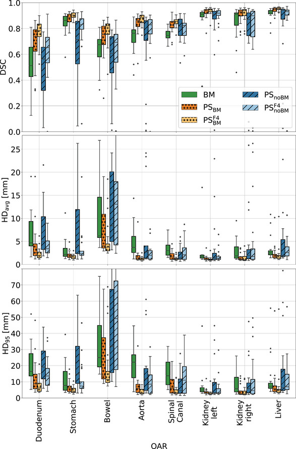
Box plots presenting DSC, 95 percentile (), and average () Hausdorff distance for the 5th fractions of the 21 test patients. For all organs‐at‐risk the performance of the following models are compared: the BMs, PS models generated by fine‐tuning the BMs with one () and five MRIs (), as well as PS models trained from scratch with one () and with 5 MRIs () of a given patient. BMs, baseline models; HD, Hausdorff distance; MRI, magnetic resonance imaging; PS, patient‐specific.
For both PS methods, whether with or without the BM, incorporating five images from a given patient led to better outcomes when compared to using only the planning MRI for training. This was particularly noticeable for models trained from scratch. Organs that benefited the most from the PS training were the aorta, bowel, duodenum, and spinal canal. In contrast, improvements for the kidneys, liver, and stomach were moderate.
The Friedman test revealed statistically significant differences among the approaches for all organs. Table S2 in the supplementary material presents the ‐values from the post‐hoc Nemenyi test. Comparison between , BM, and showed a statistically significant advantage of the former, for all OARs but the left kidney and spinal canal, where and performed equally well. In general, BMs and performed similarly and showed statistically significant differences for the left kidney, stomach, and spinal canal. Increasing the number of patient images for personalized training led to statistically significant improvements in models for all OARs but the aorta and right kidney. In models, significant improvements were noted for the duodenum and aorta.
Figure 5 presents the results of the qualitative assessment performed by a radiation oncologist. In the analysis, 70% of contours were found directly suitable for treatment adaptation (scores 0 and 1), 25% needing minor adjustments, and the remaining 5% requiring major corrections. BM‐generated delineations were also well graded, with 53% of the predictions usable right away, 26% and 16% requiring minor and major improvements, respectively. The remaining 5% were deemed not usable. Despite comparable geometric performance of the BM and , the latter were graded clearly lower with 23% of the contours usable directly, 32% and 27% requiring minor and major corrections, respectively, and 18% deemed unusable. The average scores of the three models were 1.02, 1.54, and 2.36 respectively.
FIGURE 5.

Bar plots displaying radiation oncologist's grading of predictions generated by the BMs, PS models fine‐tuning the BM with the planning MRI () and models trained from scratch with the planning MRI (). The grades range from ”ideal” to ”unusable”. BMs, baseline models; MRI, magnetic resonance imaging; PS, patient‐specific.
4. DISCUSSION
For personalized auto‐segmentation models, fine‐tuning populaiton BMs with segmented patient images ( and models) was shown to significantly improve the accuracy of BM predictions for all investigated OARs. This was demonstrated by the best DSC and HDs values, as well as qualitative assessment by a trained radiation oncologist. In fact, predictions were considered ready to use 30% more often than the contours generated by BMs.
The necessity of BMs for PS models has been investigated by training models. While they achieved geometric accuracy similar to BMs, the clinical evaluation clearly favored the latter. had only a quarter of clinically acceptable predictions and generated the highest percentage of unusable contours. Despite their relatively good overlap with the ground truth, the irregular borders of the predictions would still require tedious adjustments. In contrast, BM delineations had smoother borders and easier‐to‐correct errors, for example, misclassified volume of surrounding tissue that could be quickly deleted.
For both and models, training with more patient images further enhanced the performance of and , respectively. This was especially notable for models trained from scratch. More images not only improved DSC and HDs but also resulted in contours with smoother borders. The trend of improving PS models with more patient images (up to five fraction images) was also observed in Li et al.'s study. 15
The BMs yielded satisfactory results for most OARs, comparable to prior studies. Our DSC values for kidneys, liver, and stomach were in agreement with Fu et al.'s work, 8 but their results for bowel and duodenum surpassed ours. However, in our study we used clinical contours directly, whereas in Fu et al.'s study, the contours were refined by multiple trained professionals using dedicated software for accurate contour corrections. In comparison to Liang et al.'s study, 7 we achieved higher DSCs for kidneys but a lower one for the liver. Li et al.'s 15 results for PS models were better than ours, achieving DSCs above 0.9 for most OARs. However, their evaluation's robustness is limited by testing on only six patients. Despite all studies focused on MRIs from MR‐Linac treatments, the testing cohorts differed, introducing limitations to the comparison. Additionally, institutional guidelines, contouring styles, and the effort put into correcting the fraction contours might have influenced the ground truth quality. Therefore, the presented comparison with other studies should be taken with caution.
In this study, 2D U‐Nets were explored as potential candidates for the BMs and models, just as 3D U‐Nets were explored as candidates for models. However, the 3D BM and models showed higher DSC than their 2D counterparts, while 2D networks outperformed their 3D counterparts. Consequently, 3D architectures were selected as the final models for testing in the case of BM, , and , whereas 2D architectures were chosen for and . The superior performance of the 2D models can likely be attributed to the lower complexity of 2D models compared to their 3D counterparts in scenarios with limited data. Using 2D data effectively increases the size of the training set, as each axial slice is treated as an independent image. Selecting 2D instead of 3D networks while training with little data has also been done in the work of Fransson et al. 14 and Li et al. 15
In addition to the U‐Net architecture developed by Kerfoot et al., 21 which was used throughout this work, a preliminary study was conducted using the nnUnet‐v2 model. 28 The duodenum and aorta were included in this exploratory study, both benefiting considerably from PS training. The analysis based on the self‐configuring single‐label 3D nnUnet yielded the same conclusions: PS training enhances BM performance, and adding more images to the training set further improves outcomes. This indicates that the PS training strategies proposed in this study benefit not only a “conventional” U‐Net but also the state‐of‐the‐art nnUNet. Nevertheless, more studies are necessary to explore the advantages of this approach fully.
The predictions of models investigated in this work were also compared to predictions obtained by TotalSegmentator MRI. 29 , 30 The latter is a ready‐to‐use nnUNet that has been trained on a wide range of diagnostic MRIs from different scanners, institutions, and protocols and is therefore expected to perform well on most MR images. However, the resulting contours were worse than the predictions of all models in this study. This was partially related to differences in contouring styles, but could also be attributed to the application to an unseen MRI domain. This indicates that the TotalSegmentator MRI might require additional investigation in the future in the scope of 0.35 T MRIs from the investigated MR‐Linac, also regarding potential PS training schemes.
Not all OARs benefited equally from PS fine‐tuning or more patient images. In fact, they fell into three categories. The first included kidneys and liver, which have rather stable shapes and clear boundaries. For them, and models corrected larger BM misclassifications, but the overall improvements were moderate. The second group comprised the aorta, spinal canal, and bowel. Due to their large vertical extent, radiation oncologists segment only axial slices around the PTV. PS training encoded information on the superior‐inferior segmentation ends into each personalized model, resulting in a higher geometric agreement between the predictions and the clinical ground truth. The third subgroup included the stomach, duodenum, and again bowel, organs prone to large volume changes during the course of treatment. Notably, PS improvements were the most pronounced in this group.
In this study, we concentrated on the abdominal OARs of patients treated with MRgRT. The abdomen is known for its complexity in auto‐segmentation, making it an ideal evaluation scenario for the methods under investigation. Nevertheless, there are no conceptual limitations to employing these methods for other anatomical sites. Moreover, there are no constraints restricting their use to MRgRT. They might also be employed for other fractionated treatments, for example, in the scope of cone beam computed tomography (CBCT)‐guided adaptive radiotherapy. 31
Training of a single PS model requires less than 1 h. This is sufficiently short to be performed before the first irradiation as well as between fractions. Although preparing PS models for individual patients demands clearly more effort than training population BMs, it reduces the need for manual corrections in a critical moment, while patients are already in treatment position.
The study has its limitations. Firstly, in clinical practice, contouring radiation oncologists may not adjust OARs located further away from the PTV, considering their minimal impact on dose calculation. Consequently, while these clinical ground truth contours are sufficiently accurate for treatment adaptation, they might be suboptimal for network development. Secondly, all oncologists that generated the ground truth contours belonged to one institution. However, our previous study on OAR auto‐segmentation for prostate cancer patients 12 showed no significant differences between cohorts from different institutions, suggesting the generalizability of the presented methods. Thirdly, involving multiple radiation oncologists would enhance the robustness of the clinical evaluation. Finally, the time saved for manual corrections by using PS contours instead of the population ones has not been measured. However, the better score in the clinical evaluation suggests considerable time‐saving.
Future work directions include exploring PS transfer learning by freezing the BM parameters and adding new trainable layers. 32 Another alternative might be to use the segmented planning MRI as an additional input to help auto‐segmentation of fraction images. 33
5. CONCLUSIONS
In this study, we demonstrated the advantages of personalized segmentation models in fractionated MRgRT of the abdomen region compared to conventional BMs. Particularly, PS models generated through fine‐tuning the BM with patient data performed the best, while training from scratch performed worse than the BMs. Moreover, progressive fine‐tuning of the personalized models with new segmented fraction MRIs was shown to further enhance the performance of the models. Physician assessment showed that fine‐tuning BMs with only the planning MRI generates delineations that, in most cases, can be used directly for plan adaptation, and only a few require major corrections.
CONFLICT OF INTEREST STATEMENT
The Department of Radiation Oncology of the University Hospital of LMU Munich has research agreements with Elekta and Brainlab.
Supporting information
Supporting Information
ACKNOWLEDGMENTS
The first author wishes to thank Martin Rädler for proofreading the manuscript and discussions throughout the study. This work was funded by the Wilhelm Sander‐Stiftung (2019.162.2).
Kawula M, Marschner S, Wei C, et al. Personalized deep learning auto‐segmentation models for adaptive fractionated magnetic resonance‐guided radiation therapy of the abdomen. Med Phys. 2025;52:2295–2304. 10.1002/mp.17580
REFERENCES
- 1. Tijssen RH, Philippens ME, Paulson ES, et al. MRI commissioning of 1.5 T MR‐linac systems–a multi‐institutional study. Radiother Oncol. 2019;132:114‐120. [DOI] [PubMed] [Google Scholar]
- 2. Klüter S. Technical design and concept of a 0.35 T MR‐Linac. Clin Transl Oncol. 2019;18:98‐101. [DOI] [PMC free article] [PubMed] [Google Scholar]
- 3. Winkel D, Bol GH, Kroon PS, et al. Adaptive radiotherapy: the Elekta Unity MR‐linac concept. Clin Transl Oncol. 2019;18:54‐59. [DOI] [PMC free article] [PubMed] [Google Scholar]
- 4. Henke L, Contreras JA, Green OL, et al. Magnetic resonance image‐guided radiotherapy (MRIgRT): a 4.5‐year clinical experience. Clin Oncol. 2018;30:720‐727. [DOI] [PMC free article] [PubMed] [Google Scholar]
- 5. Corradini S, Alongi F, Andratschke N, et al.MR‐guidance in clinical reality: current treatment challenges and future perspectives. Radiat Oncol. 2019:14:1‐12. [DOI] [PMC free article] [PubMed] [Google Scholar]
- 6. Nachbar M, lo Russo M, Gani C, et al. Automatic AI‐based contouring of prostate MRI for online adaptive radiotherapy. Z Med Phys. 2023. [DOI] [PMC free article] [PubMed] [Google Scholar]
- 7. Liang F, Qian P, Su K‐H, et al. Abdominal, multi‐organ, auto‐contouring method for online adaptive magnetic resonance guided radiotherapy: an intelligent, multi‐level fusion approach. Artif Intell Med. 2018;90:34‐41. [DOI] [PubMed] [Google Scholar]
- 8. Fu Y, Mazur TR, Wu X, et al. A novel MRI segmentation method using CNN‐based correction network for MRI‐guided adaptive radiotherapy. Med Phys. 2018;45:5129‐5137. [DOI] [PubMed] [Google Scholar]
- 9. Ribeiro MF, Marschner S, Kawula M, et al. Deep learning based automatic segmentation of organs‐at‐risk for 0.35 T MRgRT of lung tumors. Radiat Oncol. 2023;18:135. [DOI] [PMC free article] [PubMed] [Google Scholar]
- 10. Harrison K, Pullen H, Welsh C, Oktay O, Alvarez‐Valle J, Jena R. Machine learning for auto‐segmentation in radiotherapy planning. Clin Oncol. 2022;34:74‐88. [DOI] [PubMed] [Google Scholar]
- 11. Hunt A, Hansen V, Oelfke U, Nill S, Hafeez S. Adaptive radiotherapy enabled by MRI guidance. Clin Oncol. 2018;30:711‐719. [DOI] [PubMed] [Google Scholar]
- 12. Kawula M, Hadi I, Nierer L, et al.Patient‐specific transfer learning for auto‐segmentation in adaptive 0.35 T MRgRT of prostate cancer: a bi‐centric evaluation. Med Phys. 2023;50:1573‐1585. [DOI] [PubMed] [Google Scholar]
- 13. Chen X, Ma X, Yan X, et al.Personalized auto‐segmentation for magnetic resonance imaging–guided adaptive radiotherapy of prostate cancer. Med Phys. 2022:49:4971‐4979. [DOI] [PubMed] [Google Scholar]
- 14. Fransson S, Tilly D, Strand R. Patient specific deep learning based segmentation for magnetic resonance guided prostate radiotherapy. Phys Imaging Radiat Oncol. 2022;23:38‐42. [DOI] [PMC free article] [PubMed] [Google Scholar]
- 15. Li Z, Zhang W, Li B, et al. Patient‐specific daily updated deep learning auto‐segmentation for MRI‐guided adaptive radiotherapy. Radiother Oncol. 2022;177:222‐230. [DOI] [PubMed] [Google Scholar]
- 16. Sharp GC, Li R, Wolfgang J, et al. Plastimatch: an open source software suite for radiotherapy image processing. In: Proceedings of the XVI'th International Conference on the use of Computers in Radiotherapy (ICCR). IEEE; 2010. [Google Scholar]
- 17. Teoh S, Ooms A, George B, et al. Evaluation of hypofractionated adaptive radiotherapy using the MR Linac in localised pancreatic cancer: protocol summary of the Emerald‐Pancreas phase 1/expansion study located at Oxford University Hospital, UK. BMJ Open. 2023;13:e068906. [DOI] [PMC free article] [PubMed] [Google Scholar]
- 18. Chuong MD, Bryant J, Mittauer KE, et al. Ablative 5‐fraction stereotactic magnetic resonance–guided radiation therapy with on‐table adaptive replanning and elective nodal irradiation for inoperable pancreas cancer. Pract Radiat Oncol. 2021;11:134‐147. [DOI] [PubMed] [Google Scholar]
- 19. Haas YP, Ludwig R, Dal Bello R, Tanadini‐Lang S, Unkelbach J. Adaptive fractionation at the MR‐linac. Phys Med Biol. 2023;68:035003. [DOI] [PubMed] [Google Scholar]
- 20. Cardoso MJ, et al. MONAI: An open‐source framework for deep learning in healthcare. arXiv preprint arXiv:2211.02701 2022.
- 21. Kerfoot E, Clough J, Oksuz I, Lee J, King AP, Schnabel JA. Left‐ventricle quantification using residual U‐Net. In: International Workshop on Statistical Atlases and Computational Models of the Heart . Springer; 2018:371‐380. [Google Scholar]
- 22. Ulyanov D, Vedaldi A, Lempitsky V. Instance Normalization: The Missing Ingredient for Fast Stylization. arXiv preprint arXiv:1607.08022 2016.
- 23. Ding B, Qian H, Zhou J. Activation functions and their characteristics in deep neural networks. In: 2018 Chinese control and decision conference (CCDC) . IEEE; 2018:1836–1841. [Google Scholar]
- 24. Bridle JS. Training stochastic model recognition algorithms as networks can lead to maximum mutual information estimation of parameters. In: Proceedings of the 2nd International Conference on Neural Information Processing Systems. MIT Press; 1990:211–217. [Google Scholar]
- 25. Milletari F, Navab N, Ahmadi S‐A. V‐net: fully convolutional neural networks for volumetric medical image segmentation. In: 2016 fourth international conference on 3D vision (3DV) . IEEE; 2016:565‐571. [Google Scholar]
- 26. Friedman M. The use of ranks to avoid the assumption of normality implicit in the analysis of variance. J Stat Data Sci Educ. 1937;32:675‐701. [Google Scholar]
- 27. Nemenyi PB. Distribution‐free multiple comparisons. Princeton University, 1963. [Google Scholar]
- 28. Isensee F, Jaeger PF, Kohl SA, Petersen J, Maier‐Hein KH. nnU‐Net: a self‐configuring method for deep learning‐based biomedical image segmentation. Nat Methods. 2021;18:203‐211. [DOI] [PubMed] [Google Scholar]
- 29. Wasserthal J, Breit H‐C, Meyer MT, et al. TotalSegmentator: robust segmentation of 104 anatomic structures in CT images. Radiology: Artificial Intelligence. 2023;5:e230235. [DOI] [PMC free article] [PubMed] [Google Scholar]
- 30. D'Antonoli TA, Berger LK, Indrakanti AK, et al. TotalSegmentator MRI: Sequence‐Independent Segmentation of 59 Anatomical Structures in MR images. 2024.
- 31. Schiff JP, Stowe HB, Price A, et al. In silico trial of computed tomography‐guided stereotactic adaptive radiation therapy (CT‐STAR) for the treatment of abdominal oligometastases. Int J Radiat Oncol Biol Phys. 2022;114:1022‐1031. [DOI] [PubMed] [Google Scholar]
- 32. Talo M, Baloglu UB, Yıldırım Ö, Acharya UR. Application of deep transfer learning for automated brain abnormality classification using MR images. Cogn Syst Res. 2019;54:176‐188. [Google Scholar]
- 33. Klymenko T, Kim ST, Lauber K, et al. Butterfly‐Net: spatial‐temporal architecture for medical image segmentation. In: 2021 IEEE 18th International Symposium on Biomedical Imaging (ISBI) . IEEE; 2021:616–620. [Google Scholar]
- 34. Pérez‐García F, Sparks R, Ourselin S. TorchIO: a Python library for efficient loading, preprocessing, augmentation and patch‐based sampling of medical images in deep learning. Comput Methods Programs Biomed. 2021:106236. [DOI] [PMC free article] [PubMed] [Google Scholar]
- 35. Kawula M, Purice D, Li M, et al. Dosimetric impact of deep learning‐based CT auto‐segmentation on radiation therapy treatment planning for prostate cancer. Radiat Oncol. 2022;17:1‐12. [DOI] [PMC free article] [PubMed] [Google Scholar]
Associated Data
This section collects any data citations, data availability statements, or supplementary materials included in this article.
Supplementary Materials
Supporting Information