The Statistics of k-mers from a Sequence Undergoing a Simple Mutation Process Without Spurious Matches

Abstract

k-mer-based methods are widely used in bioinformatics, but there are many gaps in our understanding of their statistical properties. Here, we consider the simple model where a sequence S (e.g., a genome or a read) undergoes a simple mutation process through which each nucleotide is mutated independently with some probability r, under the assumption that there are no spurious k-mer matches. How does this process affect the k-mers of S? We derive the expectation and variance of the number of mutated k-mers and of the number of islands (a maximal interval of mutated k-mers) and oceans (a maximal interval of nonmutated k-mers). We then derive hypothesis tests and confidence intervals (CIs) for r given an observed number of mutated k-mers, or, alternatively, given the Jaccard similarity (with or without MinHash). We demonstrate the usefulness of our results using a few select applications: obtaining a CI to supplement the Mash distance point estimate, filtering out reads during alignment by Minimap2, and rating long-read alignments to a de Bruijn graph by Jabba.

1. INTRODUCTION

K-Mer-based methods have become widely used, for example, for genome assembly (Bankevich et al., 2012), error correction (Salmela et al., 2017), read mapping (Jain et al., 2017; Li, 2018), variant calling (Standage et al., 2019), genotyping (Sun and Medvedev, 2018; Denti et al., 2019), database search (Solomon and Kingsford, 2016; Harris and Medvedev, 2018), metagenomic sequence comparison (Wood and Salzberg, 2014), and alignment-free sequence comparison (Song et al., 2014; Ondov et al., 2016; Sarmashghi et al., 2019). A simple but influential recent example has been the Mash distance (Ondov et al., 2016), which uses the MinHash Jaccard similarity between the sets of k-mers in two sequences to estimate their average nucleotide divergence.

Mash has been applied to determine the appropriate reference genome for in silico analyses (Schwengers et al., 2019), for genome compression (Tang et al., 2019), for clustering genomes (Brown et al., 2016; Ondov et al., 2016), and for estimating evolutionary distance from low-coverage sequencing data sets (Sarmashghi et al., 2019). k-Mer-based methods such as Mash are often faster and more practical then alignment-based methods. However, while the statistics behind sequence alignment is well understood (Gusfield, 1997), there are many gaps in our understanding of the statistics behind k-mer-based methods.

Consider the following simple mutation model and the questions it raises. There is a sequence of nucleotide S that undergoes a mutation process, through which every position is mutated with some constant probability r₁, independently of other nucleotides. In this model, we assume that S does not have any repetitive k-mers and that a mutation always results in a unique k-mer (we say that there are no spurious matches). This mutation model captures both a simple model of sequence evolution (e.g., Jukes-Cantor) and a simple model of errors generated during sequencing, under the assumptions that k is large enough and the repeat content low enough to make the effect of spurious matches negligible. It is applied to analyze algorithms, and the predictions of the model often reflect performance on real biological sequences (Ondov et al., 2016; Sarmashghi et al., 2019).

How does this simple mutation model affect the k-mers of S? This question bears resemblance, but is distinct from questions studied by Lander and Waterman (1988) and in alignment-free sequence comparison (Song et al., 2014) (we elaborate on the connection in Section 1.1). Some aspects of this question have been previously explored (Miclotte et al., 2016; Salmela et al., 2017; Wang and Au, 2020), but some very basic ones have not. For example, what is the distribution of the number of mutated k-mers? The expectation of this distribution is known and trivial to derive, but we do not know its variance.

For another example, consider that the k-mers of S fall into mutated stretches (which, inspired by the Lander/Waterman statistics, we call islands) and nonmutated stretches (which we call oceans). What is the distribution on the number of these stretches? We do not even know the expected value. We answer these and other questions in this article, with most of the results captured in Table 1.

Table 1.

The Expectation, Variances, and Hypothesis Tests Derived in This Article

Variable	Expectation	Variance	$\left(1-\alpha \right)$ interval
$N_{mut}$	Lq	$L\left(1-q\right)\left(q\left(2k+\frac{2}{r_1}-1\right)-2k\right)+f\left(r_1,k\right)$	$Lq\pm z_{\alpha }\sqrt{Var\left(N_{mut}\right)}$
$N_{isl}$	$L{r}_1\left(1-q\right)+f\left(r_1,k\right)$	$L{r}_1\left(1-q\right)\left(1-r_1\left(1-q\right)\left(2k+1\right)\right)+f\left(r_1,k\right)$	$E\left[N_{isl}\right]\pm z_{\alpha }\sqrt{Var\left(N_{isl}\right)}$
$N_{ocean}$	$L{r}_1\left(1-q\right)+f\left(r_1,k\right)$	$L{r}_1\left(1-q\right)\left(1-r_1\left(1-q\right)\left(2k+1\right)\right)+f\left(r_1,k\right)$	$E\left[N_{ocean}\right]\pm z_{\alpha }\sqrt{Var\left(N_{ocean}\right)}$
Jaccard	—	—	$\left(\frac{L-Lq-z_{\alpha }\sqrt{Var\left(N_{mut}\right)}}{L+Lq+z_{\alpha }\sqrt{Var\left(N_{mut}\right)}},\frac{L-Lq+z_{\alpha }\sqrt{Var\left(N_{mut}\right)}}{L+Lq-z_{\alpha }\sqrt{Var\left(N_{mut}\right)}}\right)$
MinHash Jaccard	—	—	See Theorem 6
$C_{ber}$	$\frac{L\left(1-q\right)\left(1+r_1\left(k-1\right)\right)+f\left(r_1,k\right)}{L+k-1}$	see Theorem 11	$E\left[C_{ber}\right]\pm z_{\alpha }\sqrt{Var\left(C_{ber}\right)}$

We use q as shorthand for as a placeholder for some function of r₁ and k that is independent of L; see the theorems for the full expressions.

We immediately apply our findings to derive hypothesis tests and confidence intervals (CIs) for r₁ from the number of observed mutated k-mers, the Jaccard similarity, and the Jaccard similarity under MinHash. Previously, none was known, even though point estimates from these had been frequently used (e.g., Mash). To do this, we observe that our random variables are m-dependent (Hoeffding et al., 1948), which, roughly speaking, means that the only dependencies involve k-mers nearby in the sequence. We apply a technique called Stein's method (Ross, 2011) to approximate these as normal variables and thereby obtain hypothesis tests and CIs.

We demonstrate the usefulness of our results using a few select applications: obtaining a CI to supplement the Mash distance point estimate (Ondov et al., 2016), filtering out reads during alignment by Minimap2 (Li, 2018), and rating long-read alignments to a de Bruijn graph by Jabba (Miclotte et al., 2016). These examples illustrate how the use of the simple mutation model and the techniques from our article could have potentially improved several widely used tools. Our technique can also be applied to new questions as they arise. Our code for computing all the intervals in this article is freely available at https://github.com/medvedevgroup/mutation-rate-intervals.

1.1. Related work

Here we give more background on how our article relates to other previous work.

1.1.1. Lander/Waterman statistics

There is a natural analogy between the stretches of mutated k-mers and the intervals covered by random clones in the work of Lander and Waterman (1988). Each error can be viewed as a random clone with fixed length k, and thus, the islands in our study correspond to “covered islands” in theirs. However, their focus was to determine how much redundancy was necessary to cover all (or most) of a genomic sequence, which would correspond to how many nucleotide mutations are needed so that most of the k-mers in the sequence are mutated. In particular, they expect average coverage of the sequence by clones to be greater than 1, while in our study we expect the corresponding value, , to be much less than 1. Thus, the approximations applied in Lander and Waterman (1988) do not hold in our case.

1.1.2. Alignment-free sequence comparison

In alignment-free analysis, two sequences are compared by comparing their respective vectors of k-mer counts (Song et al., 2014). Two such vectors can be compared in numerous ways, for example, through the D₂ similarity measure, which can be viewed as a generalization of the number of mutated k-mers we study in this article. However, in alignment-free analysis, both the underlying model and the questions studied are somewhat different. In particular, alignment-free analysis usually works with much smaller values of k, for example, $k<10$ (Wu et al., 2005). This means that most k-mers are present in a sequence, and k-mers will match between and within sequences even if they are in different locations and not evolutionarily related. Our model and questions assume that these spurious matches are background noise that can be ignored (which is justifiable for larger k), while they form a crucial component of alignment-free analysis. As a result, much of the work in measuring expectation and variance in metrics such as D₂ is done with respect to the distribution of the original sequences, rather than after a mutation process (Reinert et al., 2009; Burden et al., 2014). Even when the mutation processes have been studied, they have typically been very different from the ones we consider here (e.g., the “common motif model”; Reinert et al., 2009).

Later works (Morgenstern et al., 2015; Röhling et al., 2020) did consider the simple mutation model that we study here, although still with a small k. Sequence similarity has also been estimated using the average common substring length between two sequences (Haubold et al., 2009). This is similar to the distribution of oceans that we study in our article, but the difference is that oceans are both left- and right-maximal, while the common substrings considered by Haubold et al. (2009) and others are only right-maximal.

2. PRELIMINARIES

Let $L>0$ be a positive integer. Let $\left[L\right]$ denote the interval of integers $\left\{0,\dots ,L-1\right\}$, which intuitively captures positions along a string. Let $k>0$ be a positive integer. The k-span at position $0\le i<L$ is denoted as K_i and is the range of integers $\left[i,i+k-1\right]$ (inclusive of the endpoints). Intuitively, a k-span captures the interval of a k-mer. We think of $\left[L+k-1\right]$ as representing an interval of length $L+k-1$ that contains L k-spans. To simplify the statements of the theorems, we will in some places require that $L\ge k$ (or similar), that is, that the interval is of length at least $2k-1$. We believe this covers most practical cases of interest, but, if necessary, the results can be rederived without this assumption.

We define the simple mutation model as a random process that takes as input two integers $k>0$ and $L>0$ and a real-valued nucleotide error rate $0<r_1<1$. For every position in $\left[L+k-1\right]$, the process mutates it with probability r₁. A mutation at position i is said to mutate the k-spans $K_{max\left(0,i-k+1\right)},\dots ,K_i$. We define N_mut as a random variable, which is the number of mutated k-spans. As shorthand notation, we use to denote the probability that a k-span is mutated. Figure 1 shows an example.

FIG. 1.

An example of the simple mutation process, with $L=36$ and $k=5$. There are five nucleotides that are mutated (marked with an x). For example, the mutation at position 10 mutates the k-spans $K_6,\dots ,K_{10}$ (marked in red). Note that an isolated nucleotide mutation (e.g., at position 10) can affect up to k k-spans (e.g., $K_6,\dots ,K_{10}$), but nearby nucleotide mutations can affect the same k-span (e.g., mutation of nucleotides at positions 23 and 27 both affect $K_{23}$.) There are two islands (marked in blue) and three oceans, and $N_{mut}=21$. For example, $K_{19},\dots ,K_{34}$ is an island, and $K_{35}$ is an ocean.

The simple mutation model formalizes the notion of a string S undergoing mutations where there are no spurious matches, that is, there are no duplicate k-mers in S and a mutation always creates a unique k-mer. This is also closely related to assuming that S is random and k is large enough so that such spurious matches happen with low probability. The simple mutation model captures these scenarios by representing S using the interval $\left[L+k-1\right]$ and a k-mer as a k-span.

We can partition the sequence $K_0,\dots ,K_{L-1}$ into alternating intervals called islands and oceans. The range $i,\dots ,j$ is an island iff all $K_i,\dots ,K_j$ are mutated, and the range is maximal, that is, $K_{i-1}$ and $K_{j+1}$ are either not mutated or out of bounds. Similarly, the range is an ocean iff none of $K_i,\dots ,K_j$ is mutated, and the interval is maximal. We define N_ocean as a random variable, which is the number of oceans, and N_isl as the number of islands (Fig. 1).

Consider two strings composed of a set of k-mers A and B, respectively, and let $s\le min\left\{\left|A\right|,\left|B\right|\right\}$ be a non-negative integer. The Jaccard similarity between A and B is defined as $\frac{|A\cap B|}{|A\cup B|}$. The MinHash sketch C_S of a set C is the set of the s smallest elements in C, under a uniformly random permutation hash function. The MinHash Jaccard similarity between A and B is defined as , or, equivalently (Broder, 1997). To transplant this to our model, we define the sketching simple mutation model as an extension of the simple mutation model, with an additional non-negative integer parameter $s\le L$.

We follow the intuition of $\left[L+k-1\right]$ representing a string S with no spurious matches. For every position i, if K_i is nonmutated (respectively, mutated), we think of K_i as being shared (respectively, distinct) between the strings before and after the mutation process. Formally, let $U$ be a universe that contains an element $share{d}_i$ for every nonmutated K_i and, for every mutated K_i, contains two elements a-distinct_i and b-distinct_i. Let A be the set of all $share{d}_i$ and a-distinct_i, and let B be the set of all $share{d}_i$ and b-distinct_i. The output of the sketching simple mutation model is the MinHash Jaccard similarity between A and B, that is, 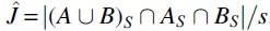. Note that the Jaccard similarity (without sketches) would, in our simple mutation model, be the ratio between the number of $share{d}_i$ and the size of $U$, which is $\frac{L-N_{mut}}{L+N_{mut}}.$

Given a distribution with a parameter of interest p, an approximate $\left(1-\alpha \right)$-CI is an interval that contains p with limiting probability $1-\alpha$. Closely related, an approximate hypothesis test with significance level $\left(1-\alpha \right)$ is an interval that contains a random variable with limiting probability $1-\alpha$. We drop the word “approximate” in the rest of the article, for brevity. We use the notation $X\in x\pm y$ to mean $X\in \left[x-y,x+y\right]$. Given $0<\alpha <1$, we define $z_{\alpha }={\Phi }^{-1}\left(1-\alpha ∕2\right)$, where ${\Phi }^{-1}$ is the inverse of the cumulative distribution function of the standard Gaussian distribution. Let $H\left(x,y,z\right)$ denote the hypergeometric distribution with population size x, y success states in population, and z trials. We define $F_n\left(a\right)=Pr\left[H\left(L+n,L-n,s\right)\ge a\right]$. Both ${\Phi }^{-1}$ and F_n can be easily evaluated in programming languages such as R or Python.

3. NUMBER OF MUTATED k-MERS: EXPECTATION AND VARIANCE

In this section, we look at the distribution of $N_{mut}$, that is, the number of mutated k-mers. The approach we take to this kind of analysis, which is standard, is to express $N_{mut}$ as a sum of indicator random variables whose pairwise dependence can be derived. Let X_i be the $0∕1$ random variable corresponding to whether or not the k-span K_i is mutated; that is, $X_i=1$ iff at least one of its nucleotides is mutated. Hence, 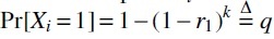. We can express $N_{mut}=\sum X_i$. By linearity of expectation, we have

$$E\left[N_{mut}\right]=E\left[\sum X_i\right]=Lq.$$ (1)

The key to the computation of variance is the joint probabilities of two k-mers being mutated.

Proof. Set $\delta =j-i$. If $\delta \ge k$, then K_i and $K_{i+\delta }$ do not overlap, and therefore, the variables X_i and $X_{i+\delta }$ are independent. Otherwise, consider three events. E₁ is the event that at least one of the positions $i,\dots ,i+\delta -1$ is mutated. E₂ is the event that none of $i,\dots ,i+\delta -1$ is mutated and one of $i+\delta ,\dots ,i+k-1$ is mutated. E₃ is the event that none of $i,\dots ,i+k-1$ is mutated. Notice that the three events form a partition of the event space and so we can write

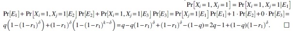
We can now compute the variance using tedious but straightforward algebraic calculations. As we show in the following section, knowing the variance allows us to obtain a CI or do a hypothesis test based on $N_{mut}$.

4. HYPOTHESIS TEST FOR M-DEPENDENT VARIABLES

Our derivations of hypothesis tests and CIs follow the strategy used for the binomials, which we now describe so as to provide intuition. In the case of estimating the success probability p of a binomial variable X when the number of trials L is known, a CI for p is called a binomial proportion CI (Casella and Berger, 2002). There are multiple ways to calculate such an interval, as described and compared in Brown et al. (2001), and we follow the approach of the Wilson score interval (Wilson, 1927). It works by first approximating the binomial with a normal distribution and then applying a standard score.

The result is that $Pr\left[|X-Lp|\le z_{\alpha }\sqrt{Var\left(X\right)}\right]=1-\alpha +\delta \left(L,p\right)$, where $Var\left(X\right)=Lp\left(1-p\right)$ and $\delta \left(L,p\right)$ is a function such that ${lim}_{L\to \infty }\delta \left(L,p\right)=0$; recall that $z_{\alpha }={\Phi }^{-1}\left(1-\alpha ∕2\right)$. This can be solved for X to obtain a hypothesis test $X\in Lp\pm z_{\alpha }\sqrt{Var\left(X\right)}$. This can be converted into a CI by finding all values of p for which $X\in Lp\pm z_{\alpha }\sqrt{Var\left(X\right)}$ holds. In the particular case of the binomial, a closed form solution is possible (Wilson, 1927), but, more generally, one can also find the solution numerically.

Although random variables such as $N_{mut}$ are not binomial, they have a specific form of dependence between the trials, which allows us to apply a similar strategy. A sequence of L random variables $X_0,\dots ,X_{L-1}$ is said to be m-dependent if there exists a bounded m (with respect to L) such that if $j-i>m$, then the two sets $\left\{X_0,\dots ,X_i\right\}$ and $\left\{X_j,\dots ,X_{L-1}\right\}$ are independent (Hoeffding et al., 1948). In other words, m-dependence says that the dependence between a sequence of random variables is limited to be within blocks of length m along the sequence.

It is known that the sum of m-dependent random variables is asymptotically normal (Hoeffding et al., 1948) and this was previously used to construct heuristic hypothesis tests and CIs (Miao and Gastwirth, 2004). Even stronger, the rate of convergence of the sum of m-dependent variables to the normal distribution is known due to a technique called Stein's method [see theorem 3.5 in Ross (2011)]. (This technique applies even to the case where m is not bounded, but that will not be the case in our article.) Here, we apply Stein's method to obtain a formally correct hypothesis test together with a rate of convergence for a sum of m-dependent (not necessarily identically distributed) Bernoulli variables.

Lemma 3. Let $X={\sum }_{i=0}^{L-1}{X}_i$ be a sum of m-dependent Bernoulli random variables, where X_i has success probability p_i. Let $\mu =\frac{1}{L}{\sum }_{i=0}^{L-1}{p}_i$, $0<\alpha <1$, and ${\sigma }_L^2=Var\left(X\right)$. Then, $Pr\left[X\ge L\mu +z_{\alpha }{\sigma }_L\right]=Pr\left[X\le L\mu -z_{\alpha }{\sigma }_L\right]=\alpha ∕2-\delta ∕2$ and

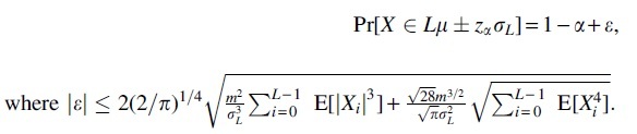
Proof. Let $Y=\left(X-L\mu \right)∕{\sigma }_L$ and let Z be a standard normal random variable. From theorem 3.6 in Ross (2011), we have $d_W\left(Y,Z\right)\le \frac{m^2}{{\sigma }_L^3}{\sum }_{i=0}^{L-1}E\left[|X_i{|}^3\right]+\frac{\sqrt{28}{m}^{3∕2}}{\sqrt{\pi }{\sigma }_L^2}\sqrt{{\sum }_{i=0}^{L-1}E\left[X_i^4\right]}=\Delta d_{max},$where d_W(.,.) denotes the Wasserstein metric. Since Z is a standard normal random variable, we have the following standard inequality between the Kolmogorov and Wasserstein metrics [see, e.g., section 3 in Ross (2011)]:

As seen, m-dependence is well suited for dealing with variables in the simple mutation model. In most natural cases, the error $\left|\delta \right|\to 0$ when $L\to \infty$, and Lemma 3 gives a hypothesis test with a significance level $1-\alpha$.

5. HYPOTHESIS TESTS FOR $N_{mut}$ AND $Ĵ$ AND CIs FOR r₁

There is a natural point estimator for r₁ using $N_{mut}$, defined as 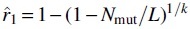This estimator is both the method of moments and the maximum likelihood estimator, meaning it has nice convergence properties as L increases (Wasserman, 2013). In this section, we extend it to a CI and a hypothesis test, both from $N_{mut}$ and $Ĵ$ (with and without sketching). In the $N_{mut}$ setting, Lemma shows that $X_0,\dots ,X_{L-1}$ are m-dependent with $m=k-1$. Hence, we can apply Lemma 3 to $N_{mut}={\sum }_{i=0}^{L-1}{X}_i.$

Corollary 4. Let , and $n_{high}=Lq+z_{\alpha }\sqrt{Var\left(N_{mut}\right)}.$ Then $Pr\left[N_{mut}\ge n_{high}\right]=Pr\left[N_{mut}\le n_{low}\right]=\alpha ∕2-\delta ∕2$ and

$$Pr\left[n_{low}\le N_{mut}\le n_{high}\right]=1-\alpha +\delta ,$$

where $\left|\delta \right|\le c∕L^{1∕4}$ and c is a constant that depends only on r₁ and k. In particular, when r₁ and k are independent of L, we have ${lim}_{L\to \infty }\left(1-\alpha +\delta \right)=1-\alpha$.

Corollary 4 gives the closed-form boundaries for a hypothesis test on N_mut. To compute a CI for q (equivalently for r₁), we can numerically find the range of q for which the observed $N_{mut}$ lies between $n_{low}$ and $n_{high}$. In other words, the upper bound on the range would be given by the value of q for which the observed $N_{mut}$ is $n_{low}$ and the lower bound by the value of q for which the observed $N_{mut}$ is $n_{high}$. These observations are made rigorous in Theorem 5. We use the notation $N_{mut}^q$ to denote $N_{mut}$ with parameter .

Theorem 5. For fixed k, r₁, and $\alpha$, for a given observed value of $N_{mut}^q,$ there exists an L large enough such that there exists a unique $q_{low}$ such that $N_{mut}^q=L{q}_{low}+z_{\alpha }\sqrt{Var\left(N_{mut}^{q_{low}}\right)}$ and a unique $q_{high}$ such that $N_{mut}^q=L{q}_{high}-z_{\alpha }\sqrt{Var\left(N_{mut}^{q_{high}}\right)}$, and

$$Pr\left[q\in \left[q_{low},q_{high}\right]\right]=1-\alpha +\delta ,$$

where $\left|\delta \right|\le c∕L^{1∕4}$ and c is a constant that depends only on r₁ and k. In particular, for fixed r₁ and k, we have ${lim}_{L\to \infty }\left(1-\alpha +\delta \right)=1-\alpha$.

Note that this theorem states that for sufficiently large L, there is a unique solution for the value of q for which the observed $N_{mut}$ is $n_{high}$ (and similarly a unique solution for the value of q for which the observed $N_{mut}$ is $n_{low}$). For small L, we have no such guarantee (although we believe the theorem holds true for all $L\ge k$); to deal with this possibility, our software verifies if the solutions are indeed unique by computing the derivative inside the proof of Theorem 5 and checking if it is positive. If it is, then the proof guarantees the solutions to be unique; if it is not, our software reports this. However, during our validations, we did not find such a case to occur.

We want to underscore how the difference between a CI and a hypothesis test is relevant in our case. A CI is useful when we have two sequences, one of which having evolved from the other and we would like to estimate their mutation rate from the number of mutated k-spans. A hypothesis test is useful when we know the mutation rate a priori, for example, the error rate of a sequencing machine. In this case, we may want to know whether a read could have been generated from a putative genome location, given the number of observed mutated k-spans. We see both applications in Section 7.

In some cases, $N_{mut}$ is not observed, but instead we observe another random variable $T=f\left(N_{mut}\right)$, where $f\left(x\right)$ is a monotone function. For example, if $f\left(x\right)=\left(L-x\right)∕\left(L+x\right)$, then T is the Jaccard similarity between the original and the mutated sequence (in our model). In this case, a hypothesis test with significance level $\alpha$ is to check if T lies between $f\left(n_{low}\right)$ and $f\left(n_{high}\right)$. In addition to the Jaccard, Lu et al. (2017) describe 14 other variables that are a function of $N_{mut}$, L, and k. These are as follows: Anderberg, Antidice, Dice, Gower, Hamman, Hamming, Kulczynski, Matching, Ochiai, Phi, Russel, Sneath, Tanimoto, and Yule. We can apply our hypothesis test to any of these variables, as long as they are monotone with respect to $N_{mut}$.

We can also use Lemma 3 as a basis for deriving a hypothesis test on $Ĵ$ in the sketching model. The proof is more involved and interesting in its own right, but is left for the Supplementary Appendix due to space constraints.

Theorem 6. Consider the sketching simple mutation model with known parameters s, k, $L\ge k$, r₁, and output $Ĵ$. Let $0<\alpha <1$ and let $m\ge 2$ be an integer. For $0\le i\le m$, let $n_l^i=Lq-z_{i∕m}\sqrt{Var\left(N_{mut}\right)}$ and $n_h^i=Lq+z_{i∕m}\sqrt{Var\left(N_{mut}\right)}$. Let

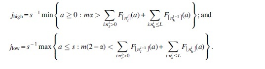
Then, assuming that r₁ and k are independent of L, and $m=o\left(L^{1∕4}\right)$,

$${lim}_{L\to \infty }Pr\left[j_{low}\le Ĵ\le j_{high}\right]=1-\alpha .$$

We can compute a CI for q from $Ĵ$ in the same manner as with Corollary 4. Let $j_{low}\left(q\right)$ and $j_{high}\left(q\right)$ be defined as in Theorem 6, but explicitly parameterized by the value of q. Then we numerically find the smallest value $0<q_{low}<1$ for which $j_{low}\left(q_{low}\right)=Ĵ$ and the largest value $0<q_{high}<1$ for which $j_{high}\left(q_{high}\right)=Ĵ$. The following theorem guarantees that $\left[q_{low},q_{high}\right]$ is a CI for q.

Theorem 7. For fixed k, r₁, $\alpha$, m, and a given observed value of $Ĵ$, there exists an L large enough such that there exist unique intervals $\left[q_{low}^{-},q_{low}^{+}\right]$ and $\left[q_{high}^{-},q_{high}^{+}\right]$ such that $q_{high}^{+}\ge q_{low}^{-}$, $j_{low}\left(\widehat{q}\right)=Ĵ$ if and only if $\widehat{q}\in \left[q_{low}^{-},q_{low}^{+}\right]$, and $j_{high}\left(\widehat{q}\right)=Ĵ$ if and only if $\widehat{q}\in \left[q_{high}^{-},q_{high}^{+}\right]$. Moreover, assuming that r₁, k, and m are independent of L, we have

$${lim}_{L\to \infty }Pr\left[q\in \left[q_{low}^{-},q_{high}^{+}\right]\right]=1-\alpha .$$

6. NUMBER OF ISLANDS AND OCEANS

In this section, we derive the expectation and variance of $N_{isl}$ and $N_{ocean}$ and the hypothesis test based on them. For $N_{isl}$, we follow the same strategy as for $N_{mut}$, namely, to express $N_{isl}$ as a sum of indicator random variables whose joint probabilities can be derived. Let us define a right border as a position i such that K_i is mutated and $K_{i+1}$ is not. We denote it by an indicator variable B_i, for $0\le i<L-1$. Let us also say that there exists an end-of-string border iff $K_{L-1}$ is mutated. We will denote this by an indicator variable Z. A right border is a position where an island ends and an ocean begins, and the end-of-string border exists if the last island is terminated not by an ocean but by the end of available nucleotides in the string to make a k-mer. The number of islands is then the number of borders, that is, $N_{isl}=Z+{\sum }_{i=0}^{L-2}{B}_i$.

To compute the expectation, observe that Z is a Bernoulli variable with parameter q. For B_i, observe that the only way that K_i is mutated while $K_{i+1}$ is not is if position i is mutated and the positions $i+1,\dots ,i+k$ are not. Therefore, $B_i\sim Bernoulli\left(r_1\left(1-q\right)\right)$. By linearity of expectation,

$$E\left[N_{isl}\right]=q+r_1\left(1-q\right)\left(L-1\right)=L{r}_1\left(1-q\right)+q-r_1\left(1-q\right).$$ (2)

Next, we derive dependencies between border variables and use them to compute the variance.

Proof. Observe that when $j-i>k$, the positions that have an effect on B_i (i.e., $K_i,\dots ,K_{i+k}$) and those that have an effect on B_j (i.e., $K_j,\dots ,K_{j+k}$) are disjoint. Hence, B_i and B_j are independent in this case. When $1\le j-i\le k$, B_i and B_j cannot co-occur. This is because $B_i=1$ implies that position j is not mutated, while $B_j=1$ implies that it is. By the same logic, Z is independent of all B_i for $0\le i\le L-2-k$. For the case when $L-2-k<i\le L-2$, $B_i=1$ implies that positions $L-1,\dots ,i+k$ are not mutated. Therefore, there is an end-of-string border when $B_i=1$ iff one of the positions $i+k+1,\dots ,L+k-2$ is mutated. Thus, .

Lemma 8 also shows that $N_{isl}$ is m-dependent, with $m=k-1$, Therefore, a hypothesis test on $N_{isl}$ can be obtained as a corollary of Lemma 3.

Corollary 10. Fix r₁ and let $0<\alpha <1$. Then, the probability that $N_{isl}\in E\left[N_{isl}\right]\pm z_{\alpha }\sqrt{Var\left(N_{isl}\right)}$ is $1-\alpha +\delta$, where $\left|\delta \right|\le c∕L^{1∕4}$ and c is a constant that depends only on r₁ and k. In particular, when r₁ and k are independent of L, we have ${lim}_{L\to \infty }\left(1-\alpha +\delta \right)=1-\alpha$.

Unlike for Corollary 4, it is not as straightforward to invert this hypothesis test into a CI for r₁, since the endpoints of the interval of $N_{isl}$ are not monotone in r₁. We therefore do not pursue this direction here. The derivation of the expectation and variance for $N_{ocean}$ are analogous and left for the Supplementary Appendix (Theorem 12). Observe that $|N_{ocean}-N_{isl}|\le 1$, so, as expected, the expectation and variance are identical to $N_{isl}$ in the higher order terms. Corollary 10 also holds for the case that n is the observed number of oceans, if we just replace $N_{isl}$ with $N_{ocean}$.

An immediate application of $N_{ocean}$ is to compute a hypothesis test for the coverage by exact regions ($C_{ber}$), a variable earlier applied to score read mappings in Miclotte et al. (2016). $C_{ber}$ is the fraction of positions in $\left[L+k-1\right]$ that lie in k-spans that are in oceans. The total number of bases in all the oceanic k-spans is the number of nonmutated k-spans plus, for each ocean, an extra $k-1$ “starter” bases. We can then write the following:

$$C_{ber}=\left(L-N_{mut}+\left(k-1\right)N_{ocean}\right)∕\left(L+k-1\right).$$

We can use the expectations and variances of $N_{mut}$ [Eq. (1) and Theorem 2] and $N_{ocean}$ (Theorem 12) to derive the expectation and variance of $C_{ber}$:

Theorem 11. $E\left[C_{ber}\right]=\frac{1-q}{L+k-1}\left(L\left(1+r_1\left(k-1\right)\right)+\left(1-r_1\right)\left(k-1\right)\right)$ and, for $L\ge k+3$, $Var\left(C_{ber}\right)=\frac{\left(1-q\right)\left(cL+d\right)}{r^2\left(L+k-1\right)}$, where

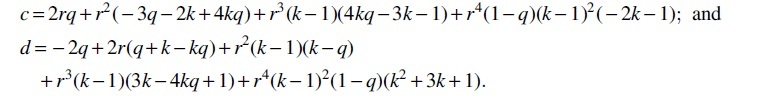
Then, observing that $C_{ber}$ is a linear combination of m-dependent variables and hence itself m-dependent, we can apply Lemma 3 and obtain that, when r₁ and k are independent of L, ${lim}_{L\to \infty }Pr\left[C_{ber}\in E\left[C_{ber}\right]\pm z_{\alpha }\sqrt{Var\left(C_{ber}\right)}\right]=1-\alpha .$

7. EMPIRICAL RESULTS AND APPLICATIONS

In this section, we evaluate the accuracy of our results and demonstrate several applications. A sanity check validation of the correctness of our formulas for $E\left[N_{mut}\right]$ and $Var\left[N_{mut}\right]$ is shown in Supplementary Appendix Table SA1, however, most of the expectation and variance formulas are evaluated indirectly through the accuracy of the corresponding CIs. We focus the evaluation on accuracy rather than run time, since calculating the CI took no more than a few seconds for most cases (the only exception was for sketch sizes of 100k or more, the evaluation took on the order of minutes). Memory use was negligible in all cases.

7.1. CIs based on $N_{mut}$

In this section, we evaluate the accuracy of the CIs produced by Corollary 4 (other CIs will be evaluated indirectly through applications). We first simulate the simple mutation model to measure the accuracy, shown in the left three groups (i.e., $L=100,1000,10,000$) of Table 2, for $\alpha =0.05$. We observe that the predicted CIs are very accurate at $L=1000$, and also accurate for smaller k and r₁ when $L=100$. Similar results hold for $\alpha =0.01$ (Supplementary Appendix Table SA2) and $\alpha =0.10$ (Supplementary Appendix Table SA3). The remainder of the cases had a CI that was too conservative; these are also the cases with some of the smallest variances (Supplementary Appendix Table SA1) and we suspect that, similar to the case of the binomial, the normal approximation of m-dependent variables deteriorates with very small variances. However, further investigation is needed.

Table 2.

The Accuracy of the Confidence Intervals for r₁ Predicted by Corollary 4, for $\alpha =0.05$ and for Various Values of L, r₁, and k (the First Three Groups) and for the Escherichia coli Sequence (the Fourth Group)

	L = 100				L = 1000				L = 10,000				Escherichia coli
r1 =	0.001	0.01	0.1	0.2	0.001	0.01	0.1	0.2	0.001	0.01	0.1	0.2	0.001	0.01	0.1	0.2
$k=100$	0.91	1.00	NA	NA	0.95	0.96	NA	NA	0.95	0.95	NA	NA	0.95	0.95	NA	NA
$k=51$	0.91	1.00	1.00	NA	0.94	0.95	0.94	NA	0.95	0.95	0.96	NA	0.95	0.95	0.95	NA
$k=21$	0.91	0.96	1.00	1.00	0.93	0.95	0.95	0.95	0.95	0.94	0.95	0.95	0.95	0.94	0.93	0.94

NA indicates that the experiment was not run; for the first three groups, we only ran on parameters where $\lceil E\left[N_{mut}\right]\rceil <L$ (otherwise they were not of interest), while for E. coli, we ran with the same range of values of r₁ and k as in the first three groups. In each cell, we report the fraction of 10,000 replicates for which the true r₁ falls into the predicted CI. For the E. coli sequence, we used the strain Shigella flexneri Shi06HN159.

CI, confidence interval.

Next, we investigate how well our predictions hold up when we simulate mutations along a real genome, where we can only observe the set of k-mers without their positions in the genome (as in alignment-free sequence comparison). We start with the Escherichia coli genome sequence and, with probability r₁, for every position, flip the nucleotide to one of three other nucleotides, chosen with equal probability. Let A and B be the set of distinct k-mers in E. coli before and after the mutation process, respectively. We let $L=\left(\left|A\right|+\left|B\right|\right)∕2$ and $n=L-|A\cap B|$. We then calculate the 95% CI for r₁ under the simple mutation model (Corollary 4) by plugging in n for $N_{mut}$. The rightmost group in Table 2 shows the accuracy of these CIs. We see that the simple mutation model we consider in this article is a good approximation to mutations along a real genome such as E. coli.

7.2. Mash distance

The Mash distance (Ondov et al., 2016) (and its follow-up modifications; Ondov et al., 2019; Sarmashghi et al., 2019) first measures the MinHash Jaccard similarity j between two sequences and then uses a formula to give a point estimate for r₁ under the assumptions of the sketching simple mutation model. While a hypothesis test was described in Ondov et al. (2016), it was only for the null model where the two sequences were unrelated. Theorem 6 allows us instead to give a CI for r₁, based on the MinHash Jaccard similarity, in the sketching simple mutation model.

Table 3 reproduces a subset of Table 1 from Ondov et al. (2016), but using CIs given by Theorem 6. For most cases, the predicted CIs are highly accurate, with an error of at most two percentage points. The three exceptions happen when s is small and q is large; in such cases, the predicted CI is too conservative (i.e., too large). In Supplementary Appendix Table SA4, we also tested the accuracy with a real E. coli genome by letting A and B be the set of distinct k-mers in the genome before and after mutations, respectively, letting $L=\left(\left|A\right|+\left|B\right|\right)∕2$ and $Ĵ=\left(\left(|A\cup B|\right)\cap A_s\cap B_s\right)∕s$, and applying Theorem 6 with those values. The accuracy is very similar to that in the simple mutation model, demonstrating that for a genome such as E. coli, the simple mutation model is a good approximation.

Table 3.

The Confidence Intervals Predicted by Theorem 6 and Their Accuracy

Sketch size	r1 = 0.05, q = 0.659			r1 = 0.15, q = 0.967			r1 = 0.25, q = 0.998
	Accuracy	Low	High	Accuracy	Low	High	Accuracy	Low	High
100	0.97	0.037	0.069	1.00	0.103	0.303	1.00	0.119	1.000
1000	0.96	0.046	0.055	0.97	0.133	0.174	1.00	0.193	0.375
10,000	0.95	0.049	0.051	0.96	0.144	0.156	0.96	0.232	0.277
100,000	0.95	0.049	0.051	0.95	0.148	0.152	0.96	0.243	0.257
1,000,000	0.94	0.050	0.050	0.95	0.149	0.151	0.96	0.247	0.253

For each sketch size and r₁ value, we show the number of trials for which the true r₁ falls within the predicted CI. The reported CI corresponds to applying Theorem 6 with $Ĵ=\frac{1-q}{1+q}$. Here, $\alpha =0.05$, $k=21$, $L=4,500,000$, and the sketch size s and r₁ are varied as shown. The number of trials for each cell is 1000, and $m=100$ for Theorem 6.

7.3. Filtering out reads during alignment to a reference

Minimap2 is a widely used long-read aligner (Li, 2018). The algorithm first picks certain k-mers in a read as seeds. Then, it identifies a region of the read and a region of the reference that potentially generated it [called a chain in Li (2018)]. Let n be the number of seeds in the read and let $m\le n$ be the number of those that exist in the reference region. Minimap2 models the error rate of the k-mers as a homogenous Poisson process and estimates the sequence divergence between the read and the reference as $\widehat{\delta }=\frac{1}{k}log\frac{n}{m}$ (which is the maximum likelihood estimator in that model). If $\widehat{\delta }$ is above a threshold, the alignment is abandoned. Li (2018) observes that due to invalid assumptions, $\widehat{\delta }$ is only approximate and can be biased, but nevertheless maintains a good correlation with the true divergence.

Using our article, we can obtain a more accurate estimate of r₁. The situation is very similar to estimating r₁ from $N_{mut}$, except that only a subset of k-spans are being “tracked.” Therefore, the maximum likelihood estimator for q is $m∕n$ and for r₁ is . Figure 2 and Supplementary Appendix Figure SA3 show the relative performance of the two estimators ($\widehat{\delta }$ and ${\widehat{r}}_1$) for sequences of different lengths, with our ${\widehat{r}}_1$ much closer to the simulated rate than $\widehat{\delta }$ in both cases.

FIG. 2.

Estimates of sequence divergence as done by mimimap2 ($\widehat{\delta }$) and by us (${\widehat{r}}_1$). Reads are simulated from a random 10 kbp sequence introducing mutations at the given r₁ rate. For each r₁ value, 100 reads are used. As in Li (2018), we use $k=15$ and, using a random hash function, identify as seeds the k-mer minimizers, one for every window of 25 k-mers. In the case when $\widehat{\delta }$ is undefined, we set $\widehat{\delta }=1$.

7.4. Evaluating an alignment of a long read to a graph

Jabba (Miclotte et al., 2016) is an error-correction algorithm for long-read data. At one stage, the algorithm evaluates whether a read is likely to have originated from a given location in the reference. Because Jabba's reference is a de Bruijn graph and not a string, it uses the specialized $C_{ber}$ score for the evaluation. In this scenario, the mutation process corresponds to sequencing errors at a known error rate r₁ and the question is whether the read is likely to have arisen through this process from the given location of the reference. The authors assume the simple mutation model and derive the expected $C_{ber}$ score as . They then give a lower rating to reads with a $C_{ber}$ score that has “significant deviation” from this expected value. It is not clear how much of a deviation is deemed to be significant or how it was calculated.

Theorem 11, which gives $E\left[C_{ber}\right]$ and $Var\left[C_{ber}\right]$, would have allowed (Miclotte et al., 2016) to take a more rigorous approach. It shows that the $C_{ber}$ expectation computed by Miclotte et al. (2016) is correct only in the limit as $L\to \infty$, while our formula is exact and closed-form. More substantially, we can make the determination of “significant deviation” more rigorous.

We regenerated Figure 2 from Miclotte et al. (2016), using the same range of values for k [called m in Miclotte et al. (2016)] and an error rate of $r_1=10\%$ as in Miclotte et al. (2016) and plotted the 95% CI as follows: $E\left[C_{ber}\right]\pm z_{0.05}\sqrt{Var\left(C_{ber}\right)}$. Figure 3 demonstrates that this range would have done a good job at capturing most of the generated reads. Table 4 gives the number of $C_{ber}$ values that fall inside of the 95% CI when using a simple mutation process with the same $r_1=10\%$ for sequences of length 10,000 for 5000 replicates, with k ranging from 5 to 50 in steps of 5, depicting good agreement between simulation and Theorem 11.

FIG. 3.

Box and whisker plot of $C_{ber}$ scores for 5000 replicates of random strings of length 10,000nt, with mutations introduced at a rate of $r_1=0.1$. The solid black line corresponds to the empirical median of $C_{ber}$, while the dashed top line corresponds to $E\left[C_{ber}\right]+z_{0.05}\sqrt{Var\left(C_{ber}\right)}$ and the bottom dot-dashed line corresponds to $E\left[C_{ber}\right]-z_{0.05}\sqrt{Var\left(C_{ber}\right)}$, both computed from Theorem 11.

Table 4.

A Total of 5000 Sequences, Each of Length 10,000nt, Underwent a Simple Mutation Process with Mutation Probability $r_1=0.1$

k-mer size	5	10	15	20	25	30	35	40	45	50
% inside CI	0.95	0.95	0.95	0.95	0.95	0.95	0.94	0.94	0.95	0.93

The percent of associated $C_{ber}$ scores that fell inside of the 95% CI as determined by Theorem 11 is shown.

8. CONCLUSION

The simple mutation model has been used broadly to model either biological mutations or sequencing errors. However, its use has usually been limited to derive the expectations of random variables, for example, the expected number of mutated k-mers. In this article, we take this a step further and show that the dependencies between indicator variables in this model (e.g., whether a k-mer at a given position is mutated) are often easy to derive and are limited to nearby locations. This limited dependency allows us to show that the sum of these indicators is approximately normal. As a result, we are able to obtain hypothesis tests and confidence tests in this model.

The most immediate application of our article is likely to compute a CI for average nucleotide identity from the MinHash sketching Jaccard. Previously, only a point estimate was available, using Mash. However, we hope that our technique can be applied by others to random variables that we did not consider. All that is needed is to derive the joint probability of the indicator variables and compute the variance. Computing the variance by hand is tedious and error-prone but can be done with the aid of software such as Mathematica.

We test the robustness of the simple mutation model in the presence of spurious matches by using a real E. coli sequence. However, we do not explore the robustness with respect to violations such as the presence of indels (which result in different string lengths) or the presence of more repeats than in E. coli. This type of robustness has already been explored in other articles that use the simple mutation model (Fan et al., 2015; Ondov et al., 2016; Sarmashghi et al., 2019). However, exploring the robustness of our CIs in downstream applications is important in future work.

On a more technical note, it would be interesting to derive more tight error bounds for our CIs, both in terms of more tightly capturing the dependencies on L, r₁, and k, and accurately tracking constants. The error bound $\delta$ that is stated in Lemma 3 is likely not tight in either respect, due to the inherent loss when transferring between the Wasserstein and Kolmogorov metrics and due to loose inequalities within the proof of theorem 3.5 in Ross (2011).

Ideally, tight error bounds would give the user a way to know, without simulations, when the CIs are accurate, in the same way that we know that the Wilson score interval for a binomial will be inaccurate when $np\left(1-p\right)$ is low. For example, it would be useful to better theoretically explain and predict which values in Table 2 deviate from 0.95.

Another practical issue is with the implementation of the algorithm to compute a CI for q from $Ĵ$. Theorem 7 guarantees that the algorithm is correct as L goes to infinity. However, the user of the algorithm will not know if L is large enough for the CI to be correct. There are several heuristic ways to check this, which we have implemented in the software: a short simulation to check the true coverage of the reported CI, a check that the sets in the definitions of $j_{high}$ and $j_{low}$ are not empty, and a check that $j_{high}$ and $j_{low}$ are monotonic with respect to q in the range $0<q<1$.

AUTHOR DISCLOSURE STATEMENT

The authors declare they have no conflicting financial interests

FUNDING INFORMATION

P.M. was supported by NSF awards 1453527 and 1439057. A.B. was supported, in part, by the NSF grant CCF-1850443. This material is based upon work supported by the National Science Foundation under Grant No. 1664803.

REFERENCES

- Bankevich, A., Nurk, S., Antipov, D., et al. 2012. SPAdes: A new genome assembly algorithm and its applications to single-cell sequencing. J. Comput. Biol. 19, 455–477. [DOI] [PMC free article] [PubMed] [Google Scholar]
- Broder, A.Z. 1997. On the resemblance and containment of documents, pp. 21–29. In: Proceedings. Compression and Complexity of SEQUENCES 1997 (Cat. No. 97TB100171). IEEE, Salerno, Italy. [Google Scholar]
- Brown, C.T., Olm, M.R., Thomas, B.C., and Banfield, J.F.. 2016. Measurement of bacterial replication rates in microbial communities. Nat. Biotechnol. 34, 1256. [DOI] [PMC free article] [PubMed] [Google Scholar]
- Brown, L.D., Cai, T.T., and DasGupta, A.. 2001. Interval estimation for a binomial proportion. Stat. Sci. 16, 101–117. [Google Scholar]
- Burden, C.J., Leopardi, P., and Forêt, S.. 2014. The distribution of word matches between markovian sequences with periodic boundary conditions. J. Comput. Biol. 21, 41–63. [DOI] [PMC free article] [PubMed] [Google Scholar]
- Casella, G., and Berger, R.L.. 2002. Statistical Inference, Vol. 2. Duxbury Pacific Grove, CA. [Google Scholar]
- Denti, L., Previtali, M., Bernardini, G., et al. 2019. MALVA: Genotyping by Mapping-free ALlele detection of known VAriants. iScience 18, 20–27. [DOI] [PMC free article] [PubMed] [Google Scholar]
- Fan, H., Ives, A.R., Surget-Groba, Y., and Cannon, C.H.. 2015. An assembly and alignment-free method of phylogeny reconstruction from next-generation sequencing data. BMC Genomics 16, 522. [DOI] [PMC free article] [PubMed] [Google Scholar]
- Gusfield, D. 1997. Algorithms on Strings, Trees and Sequences: Computer Science and Computational Biology. Cambridge University Press. [Google Scholar]
- Harris, R.S., and Medvedev, P.. 2020. Improved representation of sequence bloom trees. Bioinformatics 36, 721–727. [DOI] [PMC free article] [PubMed] [Google Scholar]
- Haubold, B., Pfaffelhuber, P., Domazet-Loso, M., and Wiehe, T.. 2009. Estimating mutation distances from unaligned genomes. J. Comput. Biol. 16, 1487–1500. [DOI] [PubMed] [Google Scholar]
- Hoeffding, W., Robbins, H., et al. 1948. The central limit theorem for dependent random variables. Duke Math. J. 15, 773–780. [Google Scholar]
- Jain, C., Dilthey, A., Koren, S., et al. 2017. A fast approximate algorithm for mapping long reads to large reference databases, pp. 66–81. In: International Conference on Research in Computational Molecular Biology. Ed: S. Cenk Sahinalp. Springer, Hongkong. [DOI] [PMC free article] [PubMed] [Google Scholar]
- Lander, E.S., and Waterman, M.S.. 1988. Genomic mapping by fingerprinting random clones: A mathematical analysis. Genomics 2, 231–239. [DOI] [PubMed] [Google Scholar]
- Li, H. 2018. Minimap2: Pairwise alignment for nucleotide sequences. Bioinformatics 34, 3094–3100. [DOI] [PMC free article] [PubMed] [Google Scholar]
- Lu, Y.Y., Tang, K., Ren, J., et al. 2017. Cafe: Accelerated alignment-free sequence analysis. Nucleic Acids Res. 45(W1), W554–W559. [DOI] [PMC free article] [PubMed] [Google Scholar]
- Miao, W., and Gastwirth, J.L.. 2004. The effect of dependence on confidence intervals for a population proportion. Am. Stat. 58, 124–130. [Google Scholar]
- Miclotte, G., Heydari, M., Demeester, P., et al. 2016. Jabba: Hybrid error correction for long sequencing reads. Algorithms Mol. Biol. 11, 1–12. [DOI] [PMC free article] [PubMed] [Google Scholar]
- Morgenstern, B., Zhu, B., Horwege, S., and Leimeister, C.A.. 2015. Estimating evolutionary distances between genomic sequences from spaced-word matches. Algorithms Mol. Biol. 10, 5. [DOI] [PMC free article] [PubMed] [Google Scholar]
- Ondov, B.D., Starrett, G.J., Sappington, A., et al. 2019. Mash Screen: High-throughput sequence containment estimation for genome discovery. Genome Biol. 20, 232. [DOI] [PMC free article] [PubMed] [Google Scholar]
- Ondov, B.D., Treangen, T.J., Melsted, P., et al. 2016. Mash: Fast genome and metagenome distance estimation using minhash. Genome Biol. 17, 132. [DOI] [PMC free article] [PubMed] [Google Scholar]
- Reinert, G., Chew, D., Sun, F., and Waterman, M.S.. 2009. Alignment-free sequence comparison (i): Statistics and power. J. Comput. Biol. 16, 1615–1634. [DOI] [PMC free article] [PubMed] [Google Scholar]
- Röhling, S., Linne, A., Schellhorn, J., et al. 2020. The number of k-mer matches between two dna sequences as a function of k and applications to estimate phylogenetic distances. PLos One 15, e0228070. [DOI] [PMC free article] [PubMed] [Google Scholar]
- Ross, N. 2011. Fundamentals of Stein's method. Probab. Surv. 8, 210–293. [Google Scholar]
- Salmela, L., Walve, R., Rivals, E., and Ukkonen, E.. 2017. Accurate self-correction of errors in long reads using de Bruijn graphs. Bioinformatics 33, 799–806. [DOI] [PMC free article] [PubMed] [Google Scholar]
- Sarmashghi, S., Bohmann, K., Gilbert, M.T.P., et al. 2019. Skmer: Assembly-free and alignment-free sample identification using genome skims. Genome Biol. 20, 1–20. [DOI] [PMC free article] [PubMed] [Google Scholar]
- Schwengers, O., Hain, T., Chakraborty, T., and Goesmann, A.. 2019. Referenceseeker: Rapid determination of appropriate reference genomes. BioRxiv. Vol. 8636. 21. [Google Scholar]
- Solomon, B., and Kingsford, C.. 2016. Fast search of thousands of short-read sequencing experiments. Nat. Biotechnol. 34, 300–302. [DOI] [PMC free article] [PubMed] [Google Scholar]
- Song, K., Ren, J., Reinert, G., et al. 2014. New developments of alignment-free sequence comparison: Measures, statistics and next-generation sequencing. Briefings Bioinf. 15, 343–353. [DOI] [PMC free article] [PubMed] [Google Scholar]
- Standage, D.S., Brown, C.T., and Hormozdiari, F.. 2019. Kevlar: A mapping-free framework for accurate discovery of de novo variants. bioRxiv. Vol. 5491. 54. [DOI] [PMC free article] [PubMed] [Google Scholar]
- Sun, C., and Medvedev, P.. 2018. Toward fast and accurate snp genotyping from whole genome sequencing data for bedside diagnostics. Bioinformatics 35, 415–420. [DOI] [PubMed] [Google Scholar]
- Tang, T., Liu, Y., Zhang, B., et al. 2019. Sketch distance-based clustering of chromosomes for large genome database compression. BMC Genomics 20, 1–9. [DOI] [PMC free article] [PubMed] [Google Scholar]
- Wang, A., and Au, K.F.. 2020. Performance difference of graph-based and alignment-based hybrid error correction methods for error-prone long reads. Genome Biol. 21, 14. [DOI] [PMC free article] [PubMed] [Google Scholar]
- Wasserman, L. 2013. All of Statistics: A Concise Course in Statistical Inference. Springer Science & Business Media, Berlin, Germany. [Google Scholar]
- Wilson, E.B. 1927. Probable inference, the law of succession, and statistical inference. J. Am. Stat. Assoc. 22, 209–212. [Google Scholar]
- Wood, D.E., and Salzberg, S.L.. 2014. Kraken: Ultrafast metagenomic sequence classification using exact alignments. Genome Biol. 15, R46. [DOI] [PMC free article] [PubMed] [Google Scholar]
- Wu, T.-J., Huang, Y.-H., and Li, L.-A.. 2005. Optimal word sizes for dissimilarity measures and estimation of the degree of dissimilarity between DNA sequences. Bioinformatics 21, 4125–4132. [DOI] [PubMed] [Google Scholar]
Associated Data
This section collects any data citations, data availability statements, or supplementary materials included in this article.