Machine learning for microbiologists

Abstract

Machine learning is increasingly important in microbiology where it is used for tasks such as predicting antibiotic resistance and associating human microbiome features with complex host diseases. The applications in microbiology are quickly expanding and the machine learning tools frequently used in basic and clinical research range from classification and regression to clustering and dimensionality reduction. In this Review, we examine the main machine learning concepts, tasks and applications that are relevant for experimental and clinical microbiologists. We provide the minimal toolbox for a microbiologist to be able to understand, interpret and use machine learning in their experimental and translational activities.

Introduction

Machine learning is a flexible set of tools for identifying patterns and relationships in complex data and for making decisions based on those data. A machine learning model can allow a vehicle to drive autonomously or use stool microbiome sequencing data to predict the presence of a disease. The experimental data collected in modern microbiology studies have reached a level of complexity where machine learning becomes necessary and an opportunity for tasks ranging from diagnostics in medicine to biomarker discovery.

Machine learning is a very broad discipline. It can be generally categorized as supervised machine learning, aimed at developing predictive models given training data where the answers are known, and unsupervised machine learning, aimed at grouping observations or creating simplified representations of major structures of the data. Examples for the former include inferring the antibiotic resistance profile of an isolate from its genome, learning whether and which components of human-associated microbial communities are involved with a given host condition or developing clinical decision support systems to recommend treatment options from pathogen or microbiome experimental data (Box 1). For unsupervised machine learning, applications range from grouping microbial genes with similar expression patterns to binning 16S rRNA gene amplicons into operational taxonomic units.

Box 1. Tasks and examples of supervised machine learning applications in microbiology.

Example 1. Machine learning to mine host–microorganism interactions

Understanding host–microorganism interactions can provide insights into molecular mechanisms underlying infectious diseases, guide discoveries of novel therapeutic modalities or lead to the repurposing of available drugs. Supervised machine learning methods such as DeNovo¹²⁷ have been developed to predict interactions between viral proteins and human proteins, irrespective of viral taxonomy and intra-species protein–protein interactions.

• Data set: VirusMentha¹²⁸, a data set containing 5,753 unique interactions between 2,357 human proteins and 453 viral proteins, covering 173 different virus species in 25 subfamilies.

• Features: protein amino acid sequences.

• Target variable to predict: whether there is an interaction between two proteins.

• Machine learning model: support vector machines.

• Training or testing sets: due to the intricacies of the experiment, the authors created subsets that contained interactions of viruses taxonomically far from those in the training set to imitate predicting a novel virus.

• Validation setting: cross-validation.

• Main result: accuracy of up to 81% and 86% when predicting protein–protein interactions of viral proteins that had no and distant sequence similarity to the ones used for model training.

Example 2. Machine learning to identify antimicrobial resistance

Early identification of the microbial species causing an infection can aid in the choice of antimicrobial therapy and dosage, which are critical for the outcome of an infection. Rapid and accurate methods are needed in the clinic, with one approach applying supervised machine learning using matrix-assisted laser desorption/ionization–time of flight (MALDI-TOF) mass spectra to predict antimicrobial resistance¹²⁹.

• Data set: 300,000 mass spectra with more than 750,000 antimicrobial resistance phenotypes derived from four medical institutions.

• Features: MALDI-TOF mass spectra profiles of clinical isolates.

• Target variable to predict: antimicrobial resistance.

• Machine learning models: logistic regression, gradient-boosted decision trees and neural networks.

• Training or testing sets: random split into 80% training and 20% testing, stratifying for antimicrobial class and the species, ensuring that multiple samples from the same patient were part of either the training or testing set, but not both.

• Validation setting: cross-validation.

• Main result: areas under the receiver operating characteristic curves between 0.80 and 0.74 for detecting antimicrobial-resistant and clinically important pathogens such as Staphylococcus aureus, Escherichia coli and Klebsiella pneumoniae.

Example 3. Machine learning to predict host disease status

The use of microbial features to predict host characteristics has been particularly successful in the study of the human microbiome, where studies have independently linked the gut microbiome to colorectal cancer and two works identified robust and reproducible associations across different cohorts and populations^25,26. These findings provide a foundation for future mechanistic studies and clinical prognostic and diagnostic tests.

• Data set: 969 faecal metagenomes from seven data sets.

• Features: presence and relative abundances of microbiome species.

• Target variable to predict: colorectal cancer versus control.

• Machine learning model: random forest and least absolute shrinkage and selection operator (LASSO).

• Training or testing sets: random split into 80/20 for training and testing sets (cross-validation); training on all but one data set and testing on the left out data set from the leave-one-data set-out (LODO) approach.

• Validation setting: cross-validation and LODO validation.

• Main result: average area under the receiver operating characteristic curve consistently above 0.80 in predicting colorectal cancer.

The importance of machine learning in microbiology is increasing and software tools are becoming more convenient and easier to adopt in this field. However, microbiologists are still being trained with little focus on quantitative and often insufficient statistical background to empower the potential of machine learning in their fields. Machine learning has complex statistical and theoretical backgrounds that will remain inaccessible to most microbiologists. However, machine learning is now structured in such a way that understanding the details of its formal foundations is not necessary to be able to use it, as long as there is a clear understanding about how to correctly apply it. The present Review has the goal of enabling microbiologists to ‘drive’ the machine learning car without necessarily knowing how the engine of the car works internally. Microbiologists with limited background in statistics and computer science should thus be able to grasp the main concepts of machine learning and include them in their activities ranging from their own experiments to the critical assessments of the work done by colleagues.

In this Review, we cover the aspects that we consider most important to enable microbiologists to use machine learning. In the first part, we introduce supervised and unsupervised machine learning techniques (with a specific focus on high-throughput microbiology settings), and we examine approaches for dimensionality reduction, as they are frequently used for exploratory microbiological investigations, and also feature selection, which is key to identifying the most relevant aspects of the microbiological phenomenon. We mention some specific machine learning algorithms of interest, but we do not aim to discuss them in depth and we refer the interested reader to more specialized literature^1–4. In the second part, we review the main aspects of model selection that are important to maximize the power of the machine learning approach, before focusing on the key practical aspects of how to evaluate a machine learning model and how to apply it in real-world scenarios minimizing underlying biases. We complete our view with several practical examples of available software implementations that can be used by microbiologists with limited computational background, discuss common pitfalls to avoid in the field and provide a practical checklist to consider when reading or assessing a machine learning-based work. The topics presented in this work will allow microbiologists to grasp the potential of machine learning in their field and enable them to consider using it in their research. Readers can expand their knowledge on the topic with other relevant reviews^5,6.

Supervised machine learning

Supervised machine learning tasks build a model that links entities or samples (for example, specific bacterial strains) with an outcome variable of interest (for example, their a priori unknown taxonomic label) using information from available experimental data (for example, known assignments of well-studied strains to their taxonomy) (Fig. 1a). Biological samples are associated both with outcomes of interest (any information about the sample and its context) and with a set of features that can be extracted from the sample itself with experimental approaches (for example, the sequence of the gene or genome of the strain, or phenotypic information obtained by in vitro experiments on the strain). Together, outcomes and features from samples are called examples and make up the ‘Training examples’ that are the input of the machine learning model (Fig. 1a). During the ‘Training phase’ the algorithm exploits the training examples to train the model that can be used to make predictions — in the ‘Prediction phase’ — about the outcome variable of new samples for which only its features are available (Fig. 1a). For example, a supervised classifier trained on known genome–species assignments that uses the presence or absence of specific genes in the genomes as features could be used to predict the species assignment of a new isolate lacking taxonomic information but for which the same types of features are available. When supervised learning uses categorical labels (for example, taxonomic labels) for the outcome variable, it is referred to as classification (Fig. 1b), whereas regression (Fig. 1c) refers to the case in which the outcome variable is a numerical continuous variable (for example, the optimal pH for a bacterium to grow). Many different methods for supervised (and unsupervised) learning are available and their diversity is enriched by the availability of many software implementations (see Supplementary Table 1 and Supplementary Box 1), allowing researchers to explore the most suitable solution for their machine learning tasks.

Fig. 1 |. General workflow and examples for machine learning applications in microbiology.

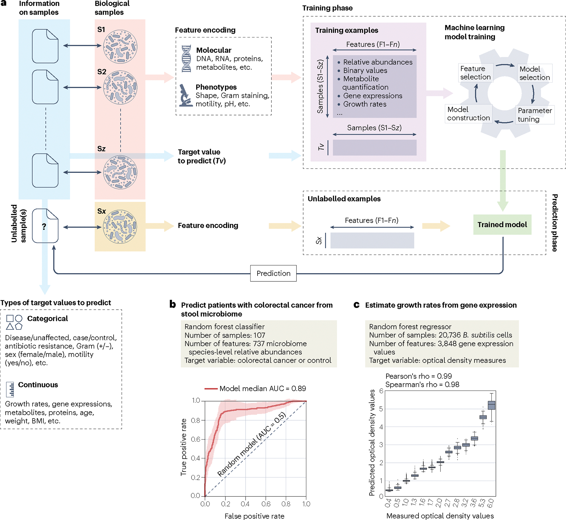
a, High-level workflow of supervised machine learning describing different types of molecular (DNA, RNA, proteins and so on) and phenotypic (morphology, motility, pH and so on) characteristics derived from biological samples (pink background) that form the set of features (indicated as F1–Fn), and target values generated from potential other information (blue background) associated with the biological samples (indicated with double-headed black arrows). The ‘Training phase’ details the input data (for example, relative abundance, metabolite quantification, gene expression and so on; violet background) and the steps that will produce the trained model, which include model selection, adjustment of the parameters, construction of the model and feature selection. The same set of features used for training the model but derived from new unseen and unlabelled biological samples (yellow background) are the input for the trained model (‘Prediction phase’) to predict the unknown corresponding outcome variable (‘?’). b, Application of supervised learning, using 737 species-level relative abundance values as input features to classify 107 stool microbiome samples into control versus colorectal cancer categories (original data from ref. 119 and available in ref. 120). This example uses the random forest classification algorithm and shows the median model’s performance (bold red line). For comparison, the dashed black line shows the performances of a random model. c, Application of supervised learning to estimate Bacillus subtilis growth rates (measured as optical density) from 3,848 gene expression values from more than 20,000 B. subtilis cells as input features⁸⁰. The example uses the random forest regression algorithm and reports the distributions of the predicted optical density values for each of the measured values. AUC, area under the curve; BMI, body mass index.

Taxonomic classification is a typical example of supervised learn ing in microbiology. The Ribosomal Database Project (RDP) classifier⁷, for instance, trains a naive Bayes model to link 16S rRNA gene sequences to their taxonomic labels and then uses the trained model to assign taxonomic labels to new 16S rRNA gene sequences. A naive Bayes classifier is a simple probabilistic model performing linear classification, and has been shown to be effective for the taxonomic classification of features coming from shotgun metagenomics^8,9. Other tools employing many different machine learning algorithms for taxonomic classification of 16S rRNA genes from isolate sequences or of 16S rRNA gene fragments from microbiome experiments have been developed for this task^10–14, including k-mer profiling and support vector machines (SVMs), frequently with better success than simple naive Bayes solutions¹⁵.

Other supervised learning approaches that use genomic data as features are those, for example, that try to predict functional or phenotypic characteristics. Several existing systems^16–18 are examples of different machine learning approaches to predict antibiotic resistance from genomic and metagenomic data^19,20. The pathogenic species Mycobacterium tuberculosis has genomic elements with a complex antimicrobial resistance evolution, and the SVM algorithm has been used to identify known and novel antimicrobial resistance genes starting from a training set of >1,500 M. tuberculosis genomes¹⁸ with experimentally tested antibiotic resistance profiles. A machine learning framework based on a set of adaptive boosting classifiers²¹ was developed to extend the identification of antimicrobial resistance to several bacterial species¹⁶, whereas the DeepARG model¹⁷ uses deep learning²² to predict antibiotic-resistant genes that can be used for the monitoring of environmental sources such as water, wastewater and food (Box 1). The prediction performance of machine learning is typically dependent on the size of the training set (assuming the quality of the data is granted), and the automatic detection of antibiotic resistance genes in Escherichia coli, for which a lot of experimental data are available, is shown to be particularly effective¹⁹. Other machine learning approaches were developed to predict less specific phenotype characteristics, including DeepBGC²³ for identifying biosynthetic gene clusters and Traitar²⁴ to predict different phenotype traits including carbon and energy sources, aerobic and spore-forming capabilities, and enzymatic activities.

Supervised learning in high-throughput microbiology settings

With the advent of high-throughput assays in microbiology such as next-generation sequencing of environmental samples (metagenomics), supervised machine learning methods are key to modelling complex and high-dimensional feature sets with phenotypes and clinical data of interest. High-dimensional quantitative features can represent a microbiological sample, for instance, by using the relative abundance of the hundreds of species present in it, the presence or absence profile of genes of a particular catalogue, or the single-nucleotide variants detected in genes of interest. Many machine learning approaches focus in this context on discriminating between cases and controls in clinical settings to inform mechanistic experiments or design new diagnostic tools (Fig. 1a,b). For instance, two large multi-data set analyses^25,26 linked colorectal cancer with the composition of the gut microbiome using random forest and sparse linear classifiers such as the least absolute shrinkage and selection operator (LASSO) (Box 1). These analyses identified a highly similar reproducible microbial signature that has been independently validated in several cohorts. It is important to underline how two different machine learning approaches achieved almost identical results, as it is usually not possible to establish which is the best machine learning approach even for a specific task, and investigators should focus more on making sure the machine learning algorithms are applied in a sound way and on clean data rather than on the choice of machine learning (sub) approaches. Microorganisms can also be found in cancer tissues, and machine learning discrimination based on microbial reads found in host sequencing efforts has a diagnostic potential²⁷.

Links between the human microbiome and six different diseases were described in a work²⁸ where more than 2,400 metagenomic samples from eight studies were used in a machine learning framework using a panel of different classifiers. An SVM algorithm trained on 50 gut microbial gene markers discriminated individuals with type 2 diabetes from healthy controls²⁹, whereas the random forest method applied on plaque microbiome profiles characterized the health status of dental implants with diagnostic and prognostic potential³⁰. The random forest method also allowed predictions of overall mortality risk by training based on human gut microbiome features³¹, and LASSO was used to identify a microbial signature from faecal microbiome samples with pancreatic cancer³². Many more examples are available as machine learning is increasingly used to estimate the strength of association between microbiomes and host characteristics such as diet, body mass index (BMI) and other cardiometabolic markers³³. Accurate prediction is an objective distinct from causal inference, another common goal in microbiome studies (see Supplementary Box 2).

Supervised machine learning in microbiology has the potential to support clinical tasks. As the microbiome has been shown to stratify, to some extent, patients with melanoma who respond to immunotherapy from non-responders^34–37, rapid metagenomic testing supported by a machine learning-based decision system could indicate the most promising treatment option in a precision medicine setting. This is a very active research area and current results have not yet reached clinical application^{34,35,38–40}. Machine learning can also support fighting the burden of infectious diseases by early identification of the infectious agents, for example by identifying microbial volatile organic compounds that discriminate between human pathogens⁴¹. Predicting the clinical success of faecal microbiota transplantation and the engraftment success of the transplant based on the characteristics of the donor sample is a similarly key medical task^39,40,42. Early results suggest that machine learning-based matching of donor-recipient individuals can expand the clinical relevance of faecal microbiota transplantation beyond the current consolidated indication for the treatment of recurrent Clostridiodes difficile infections^42–44.

Unsupervised machine learning

Machine learning is also extensively applied for tasks in which no outcome variable is available (Fig. 1a). In this ‘unsupervised’ setting, machine learning algorithms aim to find unknown structures in the data (for example, groups of similar samples) without any a priori knowledge of potential associations among samples. For example, consider isogenic bacterial cell populations in a liquid batch culture over time. The measurement of gene expression of each cell at different time points should identify cell growth phases. Unsupervised learning algorithms can partition groups of cells with similar gene expression profiles reflecting growth patterns. Similarly, a microbiologist with a large set of clonal colonies isolated from the same multi-species microbial source could use unsupervised learning on morphologies to identify strains from the same taxonomic units before focusing on specific species or functions. Unlike supervised learning, unsupervised learning can be used when labelled training sets are unavailable and when it is not known a priori what information is important. Unsupervised learning has the potential to identify novel types of information, as it is not constrained to specific predefined labels.

Clustering is an unsupervised learning method that organizes samples into groups (clusters) based on a similarity measure. The k-means and k-medoids are examples of partitional clustering methods that minimize the average distance between samples in a given cluster and the sample designated as the centre of the cluster, respectively. They both require the number of clusters (k) to be specified a priori (Fig. 2a). Applying partitional clustering suggested the presence of distinct microbial community composition types driven by the abundance of certain members of the bacterial community in the gut (enterotypes)⁴⁵ and in other human body sites⁴⁶, although others have noted a lack of defined boundaries between these clusters^47–49. Clustering on its own does not provide an algorithm to classify other samples in the future, but the clusters can be used as labels to train a supervised classifier for this purpose. However, using the same measurements (for example, taxonomic relative abundance) both to cluster samples and, then, to compute statistical tests for differences between those clusters should be avoided as this leads to inflated P values and type 1 error⁵⁰.

Fig. 2 |. Practical examples of unsupervised learning tasks.

a, k-Means is a clustering algorithm that requires an a priori number of clusters (k) into which samples are grouped. In the example, k-means with k = 2 was applied on Jaccard distances calculated using the protein content of 3,598 genomes collected by Méheust et al.¹²¹ from four published data sets^122–125 and visualized using principal component analysis (PCA). This data set includes 22,977 protein clusters representing 4,449,296 sequences from 2,321 candidate phyla radiation (CPR) genomes, 1,198 non-CPR bacterial genomes and 79 archaeal genomes. PCA is used for visualization and points are coloured according to cluster assignment. The two clusters, Cluster 1 and Cluster 2, separate according to the assigned taxonomy, with Cluster 1 containing most of the CPR genomes falling within a single cluster. Bar plot shows the fraction of genomes assigned to each cluster (top right). b, Heatmap showing the presence (yellow) and absence (black) profiles of the protein clusters (columns) across the genomes (rows). The genomes were sorted using agglomerative hierarchical clustering applied on Jaccard pairwise distances and calculated using the protein content of the genomes. Hierarchical clustering defines clusters by ‘cutting’ the hierarchical tree at a certain height. In the example, two clusters can be defined, and also in this case Cluster 1 contains most of the CPR genomes. Bar plot shows the fraction of original labels assigned to each of the 3,598 genomes separated into the two clusters as defined by the hierarchical tree (as in panel a for the clusters defined by k-means). c, PCA is a dimensionality reduction technique used to visualize high-dimensional data into a lower-dimensional space. Points represent each of the individual genomes with taxonomic kingdoms overlaid on the plot for visual exploration. Bar plot shows the first six principal components that explain most of the variance across the genomes according to their protein content (top right). d, Each component of the PCA can explain a fraction of the variance present in the data. The first two components, for instance, explain 29% of the variance, and the first principal component alone already permits partial separation of taxonomic divisions of origin of the protein clusters.

Clustering can be applied in diverse contexts using ad hoc distance functions or metrics: by defining genetic and phylogenetic distances between genomes within a single species, clustering allowed the identification of subspecies of the intestinal commensal Eubacterium rectale. This approach relied solely on uncultured metagenome-assembled genomes, highlighting differences in motility and carbohydrate utilization genes among the identified subspecies⁵¹. Hierarchical clustering methods provide additional flexibility by bypassing the need to specify the number of clusters prior to the analysis. Hierarchical clustering can use either an agglomerative approach, assigning each data point to its own cluster and merging similar pairs of clusters as the algorithm moves up the hierarchy, or a divisive one, assigning all data points to a single cluster and then partitioning clusters by least similar cluster members (Fig. 2b). Agglomerative hierarchical clustering methods applied on genetic similarity metrics have enabled the analysis of large volumes of sequence data, such as the organization of millions of prokaryotic 16S rRNA gene sequences into operational taxonomic units^52–54, or the definition of known and unknown species-level genome bins from hundreds of thousands of microbial genomes assembled directly from metagenomes⁵⁵. Cluster similarity thresholds for these tasks are typically set to 97% identity among 16S rRNA genes^56,57 to define operational taxonomic units and 95% whole-genome identity among strains to define species^55,58. Although there is multiple support, especially for the latter, investigators should be always aware that clustering thresholds cannot fully represent the nuances of microbiological entities^59,60.

Given the unprecedented increase in microbiological data generation, algorithms employing clustering concepts have been fundamental to overcoming computational challenges faced in sequencing-based molecular approaches. By reducing the redundancy of sequence sets and costs of downstream analysis and storage, greedy clustering algorithms^53,54,61 have enabled an in-depth view of the structure, diversity and function of microbial communities across habitats ranging from human body sites to the depths of the Arctic Mid-Ocean Ridge^62–64. Gene catalogues covering the genomic repertoire of microbiomes in given environments deeply rely on clustering and redundancy reduction and serve as a reference resource for the field^65–67. Sequence clustering algorithms such as MMSeq2 (ref. 68) aid in dealing with challenges faced in functional gene inference including homology detection, which is particularly relevant as sequences without annotations can range from 29% to 35% of the total depending on the environment⁶⁹. Scalability is also important, as protein catalogue searches require large computational resources and catalogues comprise more than 205 million genes from the UniProt database⁷⁰ and 170 million genes from the human gut⁷¹.

Unsupervised learning beyond clustering: dimensionality reduction

Another class of unsupervised learning algorithm aims to represent high-dimensional data (for instance, where a very high number of features are measured) in a lower-dimensional space (for example, in two dimensions that can be conveniently plotted), and is called dimensionality reduction. These techniques have become a very common approach in microbiology for data visualization, for exploratory data analysis and for reducing the dimensionality of the data for downstream machine learning tasks. Principal component analysis (PCA) is a dimensionality reduction technique based on the Euclidean distance among samples⁷² that reduces data into a lower-dimensional space of components representing groups of correlated original variables, where the first component will contain the major source of variance between samples (Fig. 2c,d). Applying PCA to the chemical property space of small molecules has shown non-obvious associations between chemical structure and differing permeabilities among bacteria, as well as differences between antibacterial compounds and non-anti-infectives⁷³. Extensions of PCA to exploit other distance metrics or dissimilarity measures among samples instead of samples’ raw variables, such as principal coordinate analysis (PCoA), have been particularly successful in the microbiome field as β-diversity estimates could be plugged directly into the dimensionality reduction procedure to reveal the overall structure of a data set^64,74–76.

Other dimensionality reduction methods try to preserve, as much as possible, the local non-linear neighbourhood structures when projecting data in low-dimensional space. Two such approaches that became very popular are t-distributed stochastic neighbour embedding (t-SNE)⁷⁷ and uniform manifold approximation and projection (UMAP)⁷⁸. These tools have been useful in elucidating cellular trajectories that reflect developmental transitions in the parasite Plasmodium berghei using single-cell RNA sequencing⁷⁹, as well as transcriptional responses to heat shock treatment and transcriptional states across Bacillus subtilis growth curves⁸⁰.

Many microbiome research reports include a two-dimensional representation of the samples based on dimensionality reduction with β-diversity metrics (for instance, micro-ecology distance functions between microbiomes). In this initial exploratory data analysis, the conditions of interest (for example, cases versus controls, or sampling of different environments) are overlaid by colouring the samples in the plot^{30,64,81–83}. Although this approach can lead to the intuitive identification of patterns in the sample space linked with relevant conditions, such findings should not be overinterpreted⁴⁸ and should be verified with statistical approaches (for example, by analysis of variance-based methods) or machine learning tools (for example, by classification or clustering analysis).

With new technologies enabling both phenotypic and genotypic profiling of single bacterial cells and communities at an unprecedented scale and depth^80,84,85, reducing the feature space of these high-dimensional data sets and grouping together similar cellular or community profiles will aid in revealing underlying biological patterns and spatiotemporal processes⁸⁶.

Feature selection and extraction

In machine learning, the main objective of feature selection is the reduction of the original number of input features that will be used for training the machine learning model. This is not to be confused with feature extraction, which refers instead to the generation of new features starting usually from a (very large) set of input features, that can be used together with the original features. In a microbiome study, for example, samples may be represented by millions of features, corresponding to the number of genes contained in microbial gene catalogues that can be found in samples⁸⁷, and it is inconvenient to maintain this high-dimensional data space for all machine learning tasks. Both feature selection and feature extraction can improve the generalization and simplification of the machine learning model by using a reduced set of input features. They can also help mitigate the ‘curse of dimensionality’ (refs. 88,89), and can improve the overall learning performance. Additionally, feature selection can have the more practical goal of reducing the computational running times of the algorithms⁹⁰. In many cases, however, feature selection has the final goal of providing a biological interpretation of the model and informing targeted follow-up experiments. As an example, the observation that Fusobacterium nucleatum and Clostridium symbiosum were among the most important features in diagnosing colorectal cancer from an analysis of the stool microbiome^91,92 promoted the use of these microbial markers in clinical use^93,94 and pointed to several mechanistic studies that partially elucidated causative links of F. nucleatum with colorectal cancer^95,96. Feature selection and feature extraction should, of course, be applied only on data of sufficient quality because this step — as well as the whole machine learning process — is subject to the general principle of ‘garbage in, garbage out’; if the input data are of poor quality, the output predictions will also be unreliable (Box 2).

Box 2. Common critical pitfalls of machine learning application in microbiological studies.

Evaluating the model.

Evaluation metrics are never general enough to express how the model performs under all conditions and it is important to understand what each metric expresses and what it hides¹⁰⁸. Unbalanced machine learning problems (that is, problems in which the samples of one class are substantially fewer than those of the other classes) should not be evaluated with the accuracy measure but, rather, with the F1 measure or the area under the precision–recall curve.

The problem of overfitting.

Selecting and tuning learning models with the appropriate complexity to fit the underlying relationship between variables requires a balance between the capacity of the model to capture this relationship and the risk of fitting the noise or the unique exceptions to each sample. Importantly, to verify model performance and avoid over-optimistic (and overfitted) estimates, an independent test set never used during the training phase should be applied to evaluate the model. In some situations, overfitting is also the consequence of an error in the design of the machine learning experiment; for example, reducing the features to the most relevant ones in a data set and then using those features to perform classification on the same data set (see Fig. 4a) is an unfortunately frequent error that completely invalidates the experiment¹³⁰.

Predictors confounded with the outcome.

Confounders are common effects of both the predictors and the outcome and can lead to spurious and biased predictions^102,131. Matching confounding variables across data sets, as well as standardization and stratification, can help mitigate this dependency. Confounders can be used in a regression analysis to produce residualized variables and used as input for prediction models.

Input training (and testing) data quality: ‘garbage in, garbage out’.

Even the best possible machine learning algorithm applied to the simplest machine learning problem cannot generate reliable predictions if the quality of the input data (samples and examples) is not sufficiently high. Errors, mislabelling, noise, file corruptions and wrong or missing pre-processing or normalizations are just some of the potential ‘data quality’ issues, and all have a crucial impact on the machine learning results. It is thus very important to assess the quality of the input data before starting any machine learning analysis.

Batch effect.

This refers to systematic variations that occur during data acquisition or processing, which can hinder the biological signal not related to biological factors, biasing the results by introducing spurious variations in a group of samples. Batch effects can be generated at different steps of the project, such as sample collection and storage, DNA extraction, library preparation, sequencing and data processing^109,132. To address batch effects, a careful study design, normalization and appropriate statistical models, as well as replication and validation cohorts, should be considered. Accounting for batch effects through blocking and randomization of samples to batches during experimental design can improve the reliability and reproducibility of results.

Low sample size.

In high-dimensional data, the greatest gains in prediction accuracy come from increasing the sample size. Leave-one-out cross-validation — in which a model is trained on all examples but one and tested on the single left-out example, and the procedure is iterated over all examples — is a common strategy to estimate performance in small data sets, although it is not free from technical issues and over-optimistic estimates.

Missing reproducibility.

Obtaining a high accuracy for a machine learning task on a data set evaluated via cross-validation or discovery/validation approaches does not usually translate into having the same performance on unseen samples from different data sets. For a model performance to be reproducible, it is key to test the model on new data sets in cross-data set evaluation and using the leave-one-data set-out (LODO) approach (Fig. 3d).

Association is not causation.

Correlation and causation are different concepts, as causes cannot be reduced to correlations, or to any other statistical relationship. Correlations are symmetrical (if ‘x’ correlates with ‘y’, then ‘y’ correlates with ‘x’), lack direction and are quantitative. By contrast, causal relationships are asymmetrical (if ‘x’ causes ‘y’, then ‘y’ is not a cause of ‘x’), directional and qualitative. Being purely observational, machine learning models are generally blind to causality because they fit underlying correlations between variables, and have been shown to be positively biased towards fitting spurious correlations instead of direct causal relationships, which can lead to biological misinterpretation and translational gaps. Causal inference is discussed in Supplementary Box 2.

There are several types of feature selection techniques. Some machine learning algorithms already embed feature selection steps, including the random forest method that provides a feature importance score, or the LASSO that constrains most regression coefficients to be exactly zero. General-purpose feature selection approaches used in the field extend to the removal of low-abundance or low-prevalence features, independently of the outcome labels⁹⁷, univariate filters⁹⁸ or sure independence screening⁹⁹. Feature selection can be combined with any learning tools by evaluating prediction performance. This involves the iterative removal or addition of features to identify those that seem redundant or provide no new information. Other feature selection approaches include recursive feature elimination based on SVMs, which was proposed for selecting genes associated with cancer tissues from micro-array data¹⁰⁰, and the minimum redundancy maximum relevance, which selects features with a weak correlation at input but a strong correlation with the target value¹⁰¹. Dimensionality reduction is a popular feature extraction approach that represents the initial feature set with a smaller number of components that do not necessarily correspond to any of the initial features. Such dimensionality reduction-based feature extraction methods are very effective when aggressive reduction of the dimensionality of data is needed and is not necessary to preserve the original features within the model.

Among the many examples available, feature selection using the LASSO was followed by SVMs to classify patients with diabetes treated with metformin, untreated patients with diabetes and non-diabetic controls¹⁰². In another work¹⁰³, three feature selection approaches were tested (ridge regression, LASSO and elastic net) in combination with several machine learning classification algorithms (Adaboost, SVM, FURIA, decision tree, Logitboost, neural network, random forest and k-NN with Logitboost) to identify disease-associated microbiome biomarkers from individuals with inflamm a tory bowel disease. Feature selection with LASSO was used also in combination with the random forest method to classify colorectal cancer using microbiome samples from the gut and oral body sites, and their combination^104,105.

Several machine learning algorithms can also output an estimation of the importance of the features in the model (for example, the random forest method provides the relative importance of each feature), which can be used to identify the features that can help explain the predictions of the model or can be followed up by targeted studies.

Model selection

The step of model selection exploits the training data to identify the best machine learning model based on the evaluation of different types of models, or across models of the same type but with different hyperparameter settings. Choosing a model with appropriate complexity and parameter settings requires balancing its capabilities of representing the underlying relationships between variables (model bias) and its sensitivity to overcome noise (model variance) that can be due to both biological and technical reasons¹⁰⁶. A machine learning model that is too simple to capture underlying relationships typically suffers from high bias and low variance (underfitting), whereas an overly complex model typically suffers from low bias and high variance (overfitting) and performs well on training data but is unlikely to perform well on new unseen data¹⁰⁷. Microbiological experiments generally produce a high number of variables that exceed the number of samples. Hence, choosing appropriate strategies to evaluate machine learning models is important to provide robust and generalizable estimations and avoid biased models⁶. Feature selection is also an important aspect of model selection, as modelling variables not associated with the target label can lead to overfitting, over-optimistic model evaluation and diminished cross-data set performance. The performance of machine learning models can be maximized by using fewer and more discriminative features, resulting in models that better generalize to new unseen data, improving both model bias and variance.

Evaluation metrics for machine learning classifiers and regressors

A machine learning model without assessment of its prediction performances on non-training data is of no value and should not be interpreted as a predictor. For machine learning evaluation, it is crucial to choose the appropriate evaluation metric for the task and select the most unbiased evaluation setting possible. Assuming to have a sufficiently large set of instances for which the target variable is known and available for evaluation (that is, not used for model training) (Fig. 3a), the choice of the performance evaluation metric depends on the goal of the machine learning model, the experimental setting and also the label type¹⁰⁸. For binary supervised problems, classifiers aim to distinguish the class of the ‘positives’ from the class of the ‘negatives’. The classification of a test sample will result in four types of outcomes: positive examples correctly classified as positives (true positives), negative examples correctly classified as negatives (true negatives), positive examples incorrectly predicted as negatives (false negatives) and negative examples incorrectly classified as positives (false positives). Based on these four outcomes, several measures of the prediction error can be calculated: accuracy, which is the fraction of correct predictions over all predictions; precision, which is the fraction of true positives over all positives; recall or sensitivity, which is the fraction of true positives over all correct predictions; and specificity, corresponding to the fraction of true negatives over all negatives. The choice of the most appropriate metric to use is context-specific. For example, in a diagnostic setting, it is usually much more problematic to misidentify a diseased individual (generating a false negative) than wrongly indicate disease (generating a false positive), and therefore recall is preferred over precision.

Fig. 3 |. Training and testing strategies for supervised machine learning model evaluation.

a,b, Supervised machine learning training (lighter boxes) and testing (bold boxes) strategies for when a single data set is available using splitting and re-sampling. Splitting one single data set into two subsets (usually with 80% and 20% of the samples, respectively) and using the larger one for model training and the smaller for model testing (panel a). k-Fold cross-validation iterates the previous splitting strategy k times (usually k = 5 or 10). It is also possible to repeat the k-fold cross-validation multiple times with random choices of the samples belonging to the folds. This strategy improves the validation power of the left-out same data set as it is less dependent on the choice of the samples in the testing set (panel b). c,d, Multi-data sets training and testing strategies using cross-data set or leave-one-data set-out (LODO) approaches. A cross-data set approach exploits one data set for training the model and the other independent data set for testing it. This is a better estimation of the generalization power of the model compared with single data set evaluations as it directly tests the performances of a different data set with potentially unavoidable differences (panel c). When more than two data sets are available, the LODO approach exploits n – 1 data sets for the training phase and uses the left-out data set for testing, repeating for all data sets. It combines the improved generalizability of the model when trained on distinct data sets with potentially different underlying differences with the comprehensive evaluation performed on multiple left-out data sets (panel d).

Many classifiers can produce, or estimate a posteriori, probabilities for the classes to predict. These probabilistic scores can be evaluated using threshold-free measures, such as the receiver operating characteristic (ROC) curve, which plots pairs of specificity and sensitivity values calculated at all possible threshold scores. The area under the ROC curve (AUC-ROC) summarizes the performances regardless of the threshold and ranges from 0.5 (random classification) to 1.0 (perfect classification). It is particularly challenging to evaluate a classifier in the presence of imbalanced classes (that is, with largely different numbers of positive and negative instances) (Box 2). In such cases, measures on binary outcomes such as the F1 score (the harmonic mean of precision and recall) or on probabilistic output such as the area under the precision–recall curve should be preferred. Regression models instead need to quantify how close the models’ predictions are to the real values, called the estimation error. Relative measures such as the coefficient of determination (R²) quantify how much variability in the dependent variable can be explained by the model, whereas absolute measures such as the (root) mean square error quantify how much the predicted results deviate from the real ones. Correlation measures are also used to evaluate the strength of the relationship between the real and the predicted values and have highlighted, for example, how well healthy plant-based foods in the habitual diet shape gut microbiome composition³³.

Approaches for unbiased evaluation of machine learning methods

The supervised machine learning classification performances should be evaluated on a test set of instances for which the target is known. The test set is usually called the validation set, as opposed to the discovery set used for training the classifier. A generalization of this approach, called k-fold cross-validation (Fig. 3b), is used especially when the number of samples is small. In k-fold cross-validation, k distinct validation sets (test folds) are selected (with or without replacement) from the only data set available and, correspondingly, k training folds are generated using all the samples not in the test folds. The supervised machine learning training and evaluation can then be performed on each training and testing fold (Fig. 3b) and the overall performance can be reported as the average and standard deviation of the test evaluation over the folds (usually 10 or 20). Importantly, when performing cross-validation for evaluating prediction performance, model selection as well as any variable selection must be performed on each training fold independently, and any cross-validation for hyperparameter tuning must be additionally nested inside each training fold.

Evaluating a supervised machine learning model via cross-validation implies that the model is tested in a setting in which, by definition, all of the samples belong to the same underlying distribution. For this reason, the performance on new unseen samples, possibly from other data sets, may be overestimated. When independent related data sets are available, it is of high relevance to validate cross-validation results in external cohorts (cross-data set validation) (Fig. 3c).

Testing the generalizability of prediction models

The accuracy of prediction models is impacted both by variance (random variability in models trained on repeated random samples) and by bias (consistent, non-random error even in large samples). Prediction models are usually created with the intention of applying them to settings beyond the one in which they were trained, and this goal of generalizability is defined as “unbiased inferences regarding a target population (beyond the subjects in the study)”¹⁰⁹. The target population likely differs from the study sample in relevant ways including geography¹¹⁰ and sociodemographics¹¹¹. Furthermore, differences in experimental protocols of independent studies may affect metagenomic quantification¹¹². On the other end, technical batch effects correlated with the outcome of interest can optimistically bias cross-validation accuracy, and correction for batch effects may not remedy this bias¹¹³. Therefore, for various reasons, accuracy estimated by splitting the available set into discovery and validation or by cross-validation may not reflect the performance expected in the generalized application of the model. This loss of accuracy in independent validation compared with cross-validation has been observed in practice, in various contexts^25,34,114. However, public availability of data from similar studies makes it possible to estimate the loss of prediction accuracy in cross-study validation compared with cross-validation^115,116, to improve the generalizability of prediction models by training on more diverse samples from independent studies and to achieve both of these goals simultaneously through the leave-one-data set-out (LODO) validation (Fig. 3d). In this scenario, each independent study is used in turn for validation whereas all other studies are used to train a model for validation on that data set. This approach was proposed for transcriptomic¹¹⁴ and microbiome studies²⁸. The microbiome-based colorectal cancer screening task has been particularly well tested in the LODO setting, showing promising clinical applications as the AUC-ROC performances on left-out data sets are predictive and consistent across populations^25,26 (Fig. 4a,b). The LODO approach has also highlighted generalization problems in other metagenomic tasks such as predicting response to immunotherapy for advanced-stage melanoma^34,35. However, in the absence of publicly available independent data sets, it can be difficult to identify the key sources of heterogeneity with the greatest impact on generalizability, as these may not be the most obvious ones known to affect the outcome of interest¹¹⁵.

Fig. 4 |. Supervised machine learning evaluation methods in a real-data example.

The diagnosis potential of colorectal cancer using only stool microbiome features with a supervised machine learning approach. a, We applied biased and unbiased training and testing strategies to detect colorectal cancer in three publicly available data sets using faecal quantitative species-level relative abundances^105,119,126. Boxplots show area under the receiver operating characteristic (ROC) curve (AUC-ROC) values obtained via training a random forest model on true labels (colorectal cancer versus control; top panel) and randomized labels (no biological signal; bottom panel). For ‘original labels’, different training and testing strategies can lead to differences in the estimated classifiers’ performances, especially when considering the model generalizability to other independent cohorts. For ‘randomized labels’, an overfitted classifier can perform better in cross-validation but will not generalize well on other independent data sets and can completely invalidate an experiment by fitting the noise of a single cohort. We show the results of model evaluation using single data sets and multi-data set training and testing strategies (as in Fig. 3). Cross-data set evaluation of unbiased classifiers achieves lower AUC-ROCs than cross-validation, which is expected given the unavoidable differences between data sets, but is a more reliable evaluation of how the model would perform on new data. To show the effects of overfitting on model performance, we ran the same analysis but pre-selected the ten species with the lowest significant unadjusted P value (P < 0.05, Wilcoxon rank-sum test). As expected, the biased classifier that would perform very well on the training set is outperformed by the unbiased one in the evaluation on test sets. Importantly, the biased classifier still performs well in cross-validation, but this is the result of overfitting as the result is also obtained when the labels are randomly assigned (and so no AUC-ROC significantly above 0.5 is possible). b, Cross-prediction matrix showing AUC-ROC mean values obtained via training a random forest model to detect colorectal cancer in four publicly available data sets using faecal quantitative species-level relative abundances^{91,105,119,126}. The matrix encompasses both single data set cross-validation and multi-data set training and testing strategies to evaluate the model’s performance. Among the described approaches, the leave-one-data set-out (LODO) AUC-ROCs should be regarded as the best possible estimations of the performance the model should achieve on new data.

Conclusions, practical recommendations and outlook

It can be challenging for scientists in life science to approach the field of machine learning due to several statistical, practical and study design aspects that are specific to machine learning and rarely considered in microbiology bachelor curricula. In this Review, we provide an overview of the main machine learning techniques, how they are applied and how they should be interpreted.

Becoming familiarized with machine learning will enable microbiology researchers to apply machine learning tools in their scientific or clinical practice. This can be achieved using available software implementations from different approaches that are progressively becoming more user-friendly and accessible (see Supplementary Table 1 and Supplementary Box 1). A strong computational background is no longer needed to use and apply machine learning methods in practice. Rather than the details of the specific machine learning algorithms, microbiologists exploring machine learning applications should focus on the general principles and guidelines outlined in this Review and on avoiding frequent potential issues affecting machine learning (Box 2) ranging from evaluation issues to study design problems. The choice of a particular machine learning algorithm should be less relevant than its correct application and usage, and different machine learning algorithms applied in the right way should provide consistent results. Understanding appropriate feature selection steps, evaluation metrics and validation settings will enable efficient choice of appropriate methods for the learning task at hand, avoiding overfitting problems and overinterpreted results. We believe the importance of these fundamentals far outweighs the incremental gains in the performance of learning tools that can typically be achieved through extensive model selection and more complex methods (Fig. 4).

A basic understanding of machine learning in microbiology is necessary not only for researchers aiming to adopt such tools but also for microbiologists to understand and critically evaluate machine learning applications performed by colleagues and other studies, to avoid drawing incorrect conclusions from wrongly applied machine learning methods. This is particularly relevant during peer review, because machine learning is now so prevalent in the scientific literature that it can be impossible to find reviewers with specific expertise in machine learning for every paper under review. In this context, a simple checklist such as the one we propose in Box 3 can be useful to remember the main aspects and potential red flags that need to be considered when assessing work done by colleagues.

Box 3. Checklist of points to verify when reading or reviewing a machine learning analysis in microbiology.

For all machine learning analyses

• Is the methodology (that is, the machine learning algorithm and the implementing software) clearly reported?

• Is the strategy for selecting models and hyper-parameters accurately described? For example, whether hyper-parameters are set to their default values, identified by validation or cross-validation on subsets of the data, or identified with other approaches.

• Are all of the data sets and all algorithms reported and linked well enough so that the analysis is fully reproducible by the reader?

For supervised learning

• Is the validation strategy clear and sound? This includes an a priori definition of a validation set, a cross-validation approach internal to the data set of interest or a cross-data set validation (see Fig. 3).

• Are validation and testing data completely hidden during model training? Watch out for information ‘leakage’ from validation to training data via imputation, normalization, batch correction, selection of relevant taxa or any use. Validation data cannot be used in any way when preparing or training the machine learning algorithm.

• Have steps been taken to ensure that the outcome of interest is not associated with any kind of batch effect one can think of?

For unsupervised learning

• Is the analysis performed without using any phenotype or outcome information, such as pre-selecting taxa associated with a phenotype or outcome of interest? Otherwise, it may better be described as (semi-)supervised.

• If semi-supervised learning is used, is it clearly stated in the work and results interpreted accordingly?

• If a claim of novel clusters is made, is it a measure of cluster strength or coherence provided at different numbers of clusters? Is a fully specified model provided that can be used to make cluster assignments in new samples? Does it provide any estimate of the uncertainty in cluster assignment?

• Is a statistical test used to show differences between clusters on variables used for the clustering? For example, if relative abundance profiles are used to cluster samples, then the average relative abundance of most species is guaranteed to differ between the clusters.

As microbiologists become more familiar with machine learning, the field will be better positioned to overcome current limitations. These span from the need for substantially larger data sets to improve predictions in clinically relevant tasks, to more precisely pinpointing microbiological aspects linked with relevant host characteristics and to the development and adoption of advanced deep learning approaches that are still suffering the high-dimensionality and low sample size of many microbiological applications¹¹⁷. The lack of precise and comprehensive metadata annotation of microbiological samples and their frequently very partial public availability are other factors currently limiting machine learning usage in this field, due to a combination of practical and ethical reasons¹¹⁸. Updated policies favouring open data sharing as well as supporting machine learning approaches such as semi-supervised learning can mitigate these issues in the future.

In this Review, we have provided an introduction to the main machine learning methods and their corresponding applications in the field of microbiology. We focused on the most widely used and relatively standard approaches to prioritize a general understanding of the principles rather than comprehensively review the last advances in the field. For these reasons, advanced machine learning settings (for example, semi-supervised learning or active learning) and techniques (for example, deep learning) are left for the interested reader to investigate in the more specialized literature.

Glossary

Accuracy

The number of correct classification predictions (true positives + true negatives) divided by the total number of predictions (true positives + true negatives + false positives + false negatives).

Area under the ROC curve

(AUC-ROC). A number between 0 and 1 that is obtained by integrating the receiver operating characteristic (ROC) curve over the different classification thresholds and that represents the ability of a binary classification model to discriminate between two classes, where 0.5 and 1 represent the random and perfect classification of the samples, respectively.

Cross-validation

An approach to provide robust performance estimates of how well the trained model generalizes on new data by splitting a data set into multiple subsets and iteratively training on some subsets and testing on the others.

Data set

A set of examples with input features and target values (if available), used to train and/or evaluate machine learning models, that can be divided into three non-overlapping subsets: training, validation and test sets. It is crucial to ensure that the same example is not present in both training and test (or validation) sets for a correct estimate of the generalizability of the learned model.

Decision tree

A non-parametric supervised learning method with a hierarchical tree structure to represent a set of if–then–else rules for different conditions. The internal nodes define conditions, and the leaves represent outputs.

Example

A processed version of the microbiological sample, including features and, possibly, targets.

Features

The microbiological data information extracted from the samples that are provided as input to the machine learning model.

Least absolute shrinkage and selection operator

(LASSO). A linear model approach that performs both variable selection and regularization (stabilization of regression coefficients) and tends to give solutions with few non-zero coefficients, to reduce the number of features and enhance the interpretability of the model.

Leave-one-data set-out

(LODO). An approach used to estimate model generalizability across data sets, that can be employed if multiple different data sets are available.

Model

A mathematical object with appropriately set parameters used to make predictions.

Naive Bayes

A supervised learning algorithm based on the application of Bayes’ theorem with the ‘naive’ assumption that all features are independent.

Neural network

A model with at least one hidden layer, a set of unobserved variables called ‘neurons’ derived from input features. Deep neural networks contain at least two hidden layers, where each neuron in a hidden layer connects to all the neurons of the next hidden layer. Combining many hidden layers and their interconnections enable modelling complex and non-linear relationships between input features and target values.

Precision

A metric for classification models that measures the fraction of true positive examples over the set of examples predicted as positives (true positives / (true positives + false positives)).

Random forest

An ensemble method that relies on a collection of independently trained decision tree models whose predictions are then aggregated to make one single prediction.

Recall

A metric for classification models that measures the fraction of true positive examples over the set of positive examples, also known as coverage (true positives / (true positives + false negatives)).

Receiver operating characteristic (ROC) curve

Generally plotted as a graph between the true positive rate and the false positive rate at different classification thresholds for evaluating a binary classification model, the curve’s shape reflects the ability of the binary classification model to separate the two classes.

Samples

Original items, for example microbiological entities, from which features data and target values are derived.

Supervised machine learning

An algorithm that trains a model to predict the target based on input features, resulting in a trained model capable of classifying new and unseen samples using the same set of features.

Support vector machines

(SVMs). A set of supervised learning prediction methods based on statistical learning theory that aims to maximize the boundary between the positive and negative classes.

Target value

A priori defined classes or quantities of microbiological interest (for example, case or control labels, Gram positive or negative staining, optimal pH values for bacterial growth) associated with examples, that are available only at training time and need to be predicted at test time from the features alone.

Test set

The (sub)set of a data set used for the final evaluation of the trained model or for which the outcomes of interest are not known and should be predicted by the trained model.

Training set

The (sub)set of a data set that is used for training a machine learning model.

Unsupervised machine learning

An algorithm that trains a model based solely on input features to derive patterns without further knowledge about the samples from which features were extracted.

Validation set

The (sub)set of a data set used to evaluate a trained model.

References

- 1.Bishop CM Pattern recognition and machine learning (Springer, 2006). [Google Scholar]
- 2.Hastie T, Tibshirani R & Friedman J The Elements of Statistical Learning: Data Mining, Inference, and Prediction 2nd edn (Springer Science & Business Media, 2009). [Google Scholar]
- 3.James G, Witten D, Hastie T & Tibshirani R An Introduction to Statistical Learning: with Applications in R (Springer Science & Business Media, 2013). [Google Scholar]
- 4.Murphy KP Probabilistic Machine Learning: Advanced Topics (MIT Press, 2022). [Google Scholar]
- 5.Goodswen SJ et al. Machine learning and applications in microbiology. FEMS Microbiol. Rev. 45, fuab015 (2021). [DOI] [PMC free article] [PubMed] [Google Scholar]
- 6. Topçuoğlu BD, Lesniak NA, Ruffin MT 4th, Wiens J & Schloss PD A framework for effective application of machine learning to microbiome-based classification problems. mBio 11, e00434–20 (2020). This work focuses on applying machine learning to microbiome data for disease prediction, highlighting the important trade-off between model complexity and interpretability, and emphasizing the need for rigorous methodology towards more reproducible machine learning usage in microbiome research.
- 7.Wang Q, Garrity GM, Tiedje JM & Cole JR Naive Bayesian classifier for rapid assignment of rRNA sequences into the new bacterial taxonomy. Appl. Environ. Microbiol. 73, 5261–5267 (2007). [DOI] [PMC free article] [PubMed] [Google Scholar]
- 8.Parks DH, MacDonald NJ & Beiko RG Classifying short genomic fragments from novel lineages using composition and homology. BMC Bioinformatics 12, 328 (2011). [DOI] [PMC free article] [PubMed] [Google Scholar]
- 9.Rosen GL, Reichenberger ER & Rosenfeld AM NBC: the Naive Bayes Classification tool webserver for taxonomic classification of metagenomic reads. Bioinformatics 27, 127–129 (2011). [DOI] [PMC free article] [PubMed] [Google Scholar]
- 10.McHardy AC, Martín HG, Tsirigos A, Hugenholtz P & Rigoutsos I Accurate phylogenetic classification of variable-length DNA fragments. Nat. Methods 4, 63–72 (2007). [DOI] [PubMed] [Google Scholar]
- 11.Patil KR, Roune L & McHardy AC The PhyloPythiaS web server for taxonomic assignment of metagenome sequences. PLoS ONE 7, e38581 (2012). [DOI] [PMC free article] [PubMed] [Google Scholar]
- 12.Gregor I, Dröge J, Schirmer M, Quince C & McHardy AC PhyloPythiaS+: a self-training method for the rapid reconstruction of low-ranking taxonomic bins from metagenomes. PeerJ 4, e1603 (2016). [DOI] [PMC free article] [PubMed] [Google Scholar]
- 13. Vervier K, Mahé P, Tournoud M, Veyrieras J-B & Vert J-P Large-scale machine learning for metagenomics sequence classification. Bioinformatics 32, 1023–1032 (2016). This work introduces a machine learning-based approach for tackling the taxonomic binning step, using a supervised approach that balances accuracy and speed and outperforms alignment-based methods.
- 14.Diaz NN, Krause L, Goesmann A, Niehaus K & Nattkemper TW TACOA — taxonomic classification of environmental genomic fragments using a kernelized nearest neighbor approach. BMC Bioinformatics 10, 56 (2009). [DOI] [PMC free article] [PubMed] [Google Scholar]
- 15.Sczyrba A et al. Critical assessment of metagenome interpretation — a benchmark of metagenomics software. Nat. Methods 14, 1063–1071 (2017). [DOI] [PMC free article] [PubMed] [Google Scholar]
- 16.Davis JJ et al. Antimicrobial resistance prediction in PATRIC and RAST. Sci. Rep. 6, 27930 (2016). [DOI] [PMC free article] [PubMed] [Google Scholar]
- 17.Arango-Argoty G et al. DeepARG: a deep learning approach for predicting antibiotic resistance genes from metagenomic data. Microbiome 6, 23 (2018). [DOI] [PMC free article] [PubMed] [Google Scholar]
- 18.Kavvas ES et al. Machine learning and structural analysis of Mycobacterium tuberculosis pan-genome identifies genetic signatures of antibiotic resistance. Nat. Commun. 9, 4306 (2018). [DOI] [PMC free article] [PubMed] [Google Scholar]
- 19.Moradigaravand D et al. Prediction of antibiotic resistance in Escherichia coli from large-scale pan-genome data. PLoS Comput. Biol. 14, e1006258 (2018). [DOI] [PMC free article] [PubMed] [Google Scholar]
- 20.Rahman SF, Olm MR, Morowitz MJ & Banfield JF Machine learning leveraging genomes from metagenomes identifies influential antibiotic resistance genes in the infant gut microbiome. mSystems 3, e00123–e00217 (2018). [DOI] [PMC free article] [PubMed] [Google Scholar]
- 21.Freund Y & Schapire RE A decision-theoretic generalization of on-line learning and an application to boosting. J. Comput. Syst. Sci. 55, 119–139 (1997). [Google Scholar]
- 22.Baldi P Deep Learning in biomedical data science. Annu. Rev. Biomed. Data Sci. 1, 181–205 (2018). [Google Scholar]
- 23.Hannigan GD et al. A deep learning genome-mining strategy for biosynthetic gene cluster prediction. Nucleic Acids Res. 47, e110 (2019). [DOI] [PMC free article] [PubMed] [Google Scholar]
- 24. Weimann A et al. From genomes to phenotypes: Traitar, the microbial trait analyzer. mSystems 1, e00101–e00116 (2016). This work uses machine learning to predict 67 microbial phenotypic traits from genome sequences, facilitating the analysis of large-scale microbial genomic data.
- 25.Thomas AM et al. Metagenomic analysis of colorectal cancer datasets identifies cross-cohort microbial diagnostic signatures and a link with choline degradation. Nat. Med. 25, 667–678 (2019). [DOI] [PMC free article] [PubMed] [Google Scholar]
- 26.Wirbel J et al. Meta-analysis of fecal metagenomes reveals global microbial signatures that are specific for colorectal cancer. Nat. Med. 25, 679–689 (2019). [DOI] [PMC free article] [PubMed] [Google Scholar]
- 27.Poore GD et al. Microbiome analyses of blood and tissues suggest cancer diagnostic approach. Nature 579, 567–574 (2020). [DOI] [PMC free article] [PubMed] [Google Scholar] [Retracted]
- 28.Pasolli E, Truong DT, Malik F, Waldron L & Segata N Machine learning meta- analysis of large metagenomic datasets: tools and biological insights. PLoS Comput. Biol. 12, e1004977 (2016). [DOI] [PMC free article] [PubMed] [Google Scholar]
- 29.Qin J et al. A metagenome-wide association study of gut microbiota in type 2 diabetes. Nature 490, 55–60 (2012). [DOI] [PubMed] [Google Scholar]
- 30.Ghensi P et al. Strong oral plaque microbiome signatures for dental implant diseases identified by strain-resolution metagenomics. NPJ Biofilms Microbiomes 6, 47 (2020). [DOI] [PMC free article] [PubMed] [Google Scholar]
- 31.Salosensaari A et al. Taxonomic signatures of cause-specific mortality risk in human gut microbiome. Nat. Commun. 12, 2671 (2021). [DOI] [PMC free article] [PubMed] [Google Scholar]
- 32.Kartal E et al. A faecal microbiota signature with high specificity for pancreatic cancer. Gut 71, 1359–1372 (2022). [DOI] [PMC free article] [PubMed] [Google Scholar]
- 33.Asnicar F et al. Microbiome connections with host metabolism and habitual diet from 1,098 deeply phenotyped individuals. Nat. Med. 21, 321–332 (2021). [DOI] [PMC free article] [PubMed] [Google Scholar]
- 34.Lee KA et al. Cross-cohort gut microbiome associations with immune checkpoint inhibitor response in advanced melanoma. Nat. Med. 28, 535–544 (2022). [DOI] [PMC free article] [PubMed] [Google Scholar]
- 35.McCulloch JA et al. Intestinal microbiota signatures of clinical response and immune-related adverse events in melanoma patients treated with anti-PD-1. Nat. Med. 28, 545–556 (2022). [DOI] [PMC free article] [PubMed] [Google Scholar]
- 36.Routy B et al. Gut microbiome influences efficacy of PD-1-based immunotherapy against epithelial tumors. Science 359, 91–97 (2018). [DOI] [PubMed] [Google Scholar]
- 37.Gopalakrishnan V et al. Gut microbiome modulates response to anti–PD-1 immunotherapy in melanoma patients. Science 359, 97–103 (2018). [DOI] [PMC free article] [PubMed] [Google Scholar]
- 38.Derosa L et al. Intestinal Akkermansia muciniphila predicts overall survival in advanced non-small cell lung cancer patients treated with anti-PD-1 antibodies: results a phase II study. J. Clin. Orthod. 39, 9019–9019 (2021). [Google Scholar]
- 39.Davar D et al. Fecal microbiota transplant overcomes resistance to anti-PD-1 therapy in melanoma patients. Science 371, 595–602 (2021). [DOI] [PMC free article] [PubMed] [Google Scholar]
- 40.Baruch EN et al. Fecal microbiota transplant promotes response in immunotherapy-refractory melanoma patients. Science 371, 602–609 (2021). [DOI] [PubMed] [Google Scholar]
- 41.Palma SICJ et al. Machine learning for the meta-analyses of microbial pathogens’ volatile signatures. Sci. Rep. 8, 3360 (2018). [DOI] [PMC free article] [PubMed] [Google Scholar]
- 42. Ianiro G et al. Variability of strain engraftment and predictability of microbiome composition after fecal microbiota transplantation across different diseases. Nat. Med. 28, 1913–1923 (2022). This study uses machine learning to develop predictive models for selecting optimal donors for faecal microbiota transplantation, making personalized microbiome-targeted treatments more effective.
- 43.Smillie CS et al. Strain tracking reveals the determinants of bacterial engraftment in the human gut following fecal microbiota transplantation. Cell Host Microbe 23, 229–240.e5 (2018). [DOI] [PMC free article] [PubMed] [Google Scholar]
- 44.Schmidt TSB et al. Drivers and determinants of strain dynamics following fecal microbiota transplantation. Nat. Med. 28, 1902–1912 (2022). [DOI] [PMC free article] [PubMed] [Google Scholar]
- 45.Arumugam M et al. Enterotypes of the human gut microbiome. Nature 473, 174–180 (2011). [DOI] [PMC free article] [PubMed] [Google Scholar]
- 46.Ravel J et al. Vaginal microbiome of reproductive-age women. Proc. Natl Acad. Sci. USA 108, 4680–4687 (2011). [DOI] [PMC free article] [PubMed] [Google Scholar]
- 47.Koren O et al. A guide to enterotypes across the human body: meta-analysis of microbial community structures in human microbiome datasets. PLoS Comput. Biol. 9, e1002863 (2013). [DOI] [PMC free article] [PubMed] [Google Scholar]
- 48.Knights D et al. Rethinking ‘enterotypes’. Cell Host Microbe 16, 433–437 (2014). [DOI] [PMC free article] [PubMed] [Google Scholar]
- 49.Costea PI et al. Enterotypes in the landscape of gut microbial community composition. Nat. Microbiol. 3, 8–16 (2018). [DOI] [PMC free article] [PubMed] [Google Scholar]
- 50.Gao LL, Bien J & Witten D Selective inference for hierarchical clustering. J. Am. Stat. Assoc. 10.1080/01621459.2022.2116331 (2022). [DOI] [PMC free article] [PubMed] [Google Scholar]
- 51.Karcher N et al. Analysis of 1321 Eubacterium rectale genomes from metagenomes uncovers complex phylogeographic population structure and subspecies functional adaptations. Genome Biol. 21, 138 (2020). [DOI] [PMC free article] [PubMed] [Google Scholar]
- 52.Hamady M & Knight R Microbial community profiling for human microbiome projects: tools, techniques, and challenges. Genome Res 19, 1141–1152 (2009). [DOI] [PMC free article] [PubMed] [Google Scholar]
- 53.Edgar RC Search and clustering orders of magnitude faster than BLAST. Bioinformatics 26, 2460–2461 (2010). [DOI] [PubMed] [Google Scholar]
- 54.Rognes T, Flouri T, Nichols B, Quince C & Mahé F VSEARCH: a versatile open source tool for metagenomics. PeerJ 4, e2584 (2016). [DOI] [PMC free article] [PubMed] [Google Scholar]
- 55.Pasolli E et al. Extensive unexplored human microbiome diversity revealed by over 150,000 genomes from metagenomes spanning age, geography, and lifestyle. Cell 176, 1–14 (2019). [DOI] [PMC free article] [PubMed] [Google Scholar]
- 56.Konstantinidis KT & Tiedje JM Genomic insights that advance the species definition for prokaryotes. Proc. Natl Acad. Sci. USA 102, 2567–2572 (2005). [DOI] [PMC free article] [PubMed] [Google Scholar]
- 57.Nguyen N-P, Warnow T, Pop M & White B A perspective on 16S rRNA operational taxonomic unit clustering using sequence similarity. NPJ Biofilms Microbiomes 2, 16004 (2016). [DOI] [PMC free article] [PubMed] [Google Scholar]
- 58.Jain C, Rodriguez-R LM, Phillippy AM, Konstantinidis KT & Aluru S High throughput ANI analysis of 90K prokaryotic genomes reveals clear species boundaries. Nat. Commun. 9, 5114 (2018). [DOI] [PMC free article] [PubMed] [Google Scholar]
- 59.Murray CS, Gao Y & Wu M Re-evaluating the evidence for a universal genetic boundary among microbial species. Nat. Commun. 12, 4059 (2021). [DOI] [PMC free article] [PubMed] [Google Scholar]
- 60.Rodriguez-R LM, Jain C, Conrad RE, Aluru S & Konstantinidis KT Reply to: ‘Re-evaluating the evidence for a universal genetic boundary among microbial species’. Nat. Commun. 12, 4060 (2021). [DOI] [PMC free article] [PubMed] [Google Scholar]
- 61.Li W & Godzik A cd-hit: a fast program for clustering and comparing large sets of protein or nucleotide sequences. Bioinformatics 22, 1658–1659 (2006). [DOI] [PubMed] [Google Scholar]
- 62.Bahram M et al. Structure and function of the global topsoil microbiome. Nature 560, 233–237 (2018). [DOI] [PubMed] [Google Scholar]
- 63.Spang A et al. Complex archaea that bridge the gap between prokaryotes and eukaryotes. Nature 521, 173–179 (2015). [DOI] [PMC free article] [PubMed] [Google Scholar]
- 64.Human Microbiome Project Consortium. Structure, function and diversity of the healthy human microbiome. Nature 486, 207–214 (2012). [DOI] [PMC free article] [PubMed] [Google Scholar]
- 65.Xiao L et al. A catalog of the mouse gut metagenome. Nat. Biotechnol. 33, 1103–1108 (2015). [DOI] [PubMed] [Google Scholar]
- 66.Qin J et al. A human gut microbial gene catalogue established by metagenomic sequencing. Nature 464, 59–65 (2010). [DOI] [PMC free article] [PubMed] [Google Scholar]
- 67.Chen C et al. Expanded catalog of microbial genes and metagenome-assembled genomes from the pig gut microbiome. Nat. Commun. 12, 1106 (2021). [DOI] [PMC free article] [PubMed] [Google Scholar]
- 68.Steinegger M & Söding J MMseqs2 enables sensitive protein sequence searching for the analysis of massive data sets. Nat. Biotechnol. 35, 1026–1028 (2017). [DOI] [PubMed] [Google Scholar]
- 69.Vanni C et al. Unifying the known and unknown microbial coding sequence space. eLife 11, e67667 (2022). [DOI] [PMC free article] [PubMed] [Google Scholar]
- 70.Apweiler R et al. UniProt: the universal protein knowledgebase. Nucleic Acids Res. 32, D115–D119 (2004). [DOI] [PMC free article] [PubMed] [Google Scholar]
- 71.Almeida A et al. A unified catalog of 204,938 reference genomes from the human gut microbiome. Nat. Biotechnol. 39, 105–114 (2021). [DOI] [PMC free article] [PubMed] [Google Scholar]
- 72.Abdi H & Williams LJ Principal component analysis. Wiley Interdiscip. Rev. Comput. Stat. 2, 433–459 (2010). [Google Scholar]
- 73.Davis TD, Gerry CJ & Tan DS General platform for systematic quantitative evaluation of small-molecule permeability in bacteria. ACS Chem. Biol. 9, 2535–2544 (2014). [DOI] [PMC free article] [PubMed] [Google Scholar]
- 74.Suchodolski JS et al. The fecal microbiome in dogs with acute diarrhea and idiopathic inflammatory bowel disease. PLoS ONE 7, e51907 (2012). [DOI] [PMC free article] [PubMed] [Google Scholar]
- 75.Mishiro T et al. Oral microbiome alterations of healthy volunteers with proton pump inhibitor. J. Gastroenterol. Hepatol. 33, 1059–1066 (2018). [DOI] [PubMed] [Google Scholar]
- 76.Vázquez-Baeza Y, Pirrung M, Gonzalez A & Knight R EMPeror: a tool for visualizing high-throughput microbial community data. Gigascience 2, 16 (2013). [DOI] [PMC free article] [PubMed] [Google Scholar]
- 77.van der Maaten L & Hinton G Visualizing data using t-SNE. J. Mach. Learn. Res. 9, 2579–2605 (2008). [Google Scholar]
- 78.Becht E et al. Dimensionality reduction for visualizing single-cell data using UMAP. Nat. Biotechnol. 37, 38–44 (2018). [DOI] [PubMed] [Google Scholar]
- 79.Howick VM et al. The Malaria Cell Atlas: single parasite transcriptomes across the complete Plasmodium life cycle. Science 365, eaaw2619 (2019). [DOI] [PMC free article] [PubMed] [Google Scholar]
- 80.Kuchina A et al. Microbial single-cell RNA sequencing by split-pool barcoding. Science 371, eaba5257 (2021). [DOI] [PMC free article] [PubMed] [Google Scholar]
- 81.Yatsunenko T et al. Human gut microbiome viewed across age and geography. Nature 486, 222–227 (2012). [DOI] [PMC free article] [PubMed] [Google Scholar]
- 82.Rousk J et al. Soil bacterial and fungal communities across a pH gradient in an arable soil. ISME J. 4, 1340–1351 (2010). [DOI] [PubMed] [Google Scholar]
- 83.Aagaard K et al. A metagenomic approach to characterization of the vaginal microbiome signature in pregnancy. PLoS ONE 7, e36466 (2012). [DOI] [PMC free article] [PubMed] [Google Scholar]
- 84.Blattman SB, Jiang W, Oikonomou P & Tavazoie S Prokaryotic single-cell RNA sequencing by in situ combinatorial indexing. Nat. Microbiol. 5, 1192–1201 (2020). [DOI] [PMC free article] [PubMed] [Google Scholar]
- 85.Jeckel H & Drescher K Advances and opportunities in image analysis of bacterial cells and communities. FEMS Microbiol. Rev. 45, fuaa062 (2020). [DOI] [PMC free article] [PubMed] [Google Scholar]
- 86.Geier B et al. Spatial metabolomics of in situ host–microbe interactions at the micrometre scale. Nat. Microbiol. 5, 498–510 (2020). [DOI] [PubMed] [Google Scholar]
- 87.Le Chatelier E et al. Richness of human gut microbiome correlates with metabolic markers. Nature 500, 541–546 (2013). [DOI] [PubMed] [Google Scholar]
- 88.Li H Microbiome, metagenomics, and high-dimensional compositional data analysis. Annu. Rev. Stat. Appl. 2, 73–94 (2015). [Google Scholar]
- 89.Gloor GB, Macklaim JM, Pawlowsky-Glahn V & Egozcue JJ Microbiome datasets are compositional: and this is not optional. Front. Microbiol. 8, 2224 (2017). [DOI] [PMC free article] [PubMed] [Google Scholar]
- 90.Bermingham ML et al. Application of high-dimensional feature selection: evaluation for genomic prediction in man. Sci. Rep. 5, 10312 (2015). [DOI] [PMC free article] [PubMed] [Google Scholar]
- 91.Zeller G et al. Potential of fecal microbiota for early-stage detection of colorectal cancer. Mol. Syst. Biol. 10, 766 (2014). [DOI] [PMC free article] [PubMed] [Google Scholar]
- 92.Zackular JP, Rogers MAM, Ruffin MT 4th & Schloss PD The human gut microbiome as a screening tool for colorectal cancer. Cancer Prev. Res. 7, 1112–1121 (2014). [DOI] [PMC free article] [PubMed] [Google Scholar]
- 93.Wong SH et al. Quantitation of faecal Fusobacterium improves faecal immunochemical test in detecting advanced colorectal neoplasia. Gut 66, 1441–1448 (2017). [DOI] [PMC free article] [PubMed] [Google Scholar]
- 94.Xie Y-H et al. Fecal Clostridium symbiosum for noninvasive detection of early and advanced colorectal cancer: test and validation studies. EBioMedicine 25, 32–40 (2017). [DOI] [PMC free article] [PubMed] [Google Scholar]
- 95.Kostic AD et al. Fusobacterium nucleatum potentiates intestinal tumorigenesis and modulates the tumor-immune microenvironment. Cell Host Microbe 14, 207–215 (2013). [DOI] [PMC free article] [PubMed] [Google Scholar]
- 96.Rubinstein MR et al. Fusobacterium nucleatum promotes colorectal carcinogenesis by modulating E-cadherin/β-catenin signaling via its FadA adhesin. Cell Host Microbe 14, 195–206 (2013). [DOI] [PMC free article] [PubMed] [Google Scholar]
- 97.Bourgon R, Gentleman R & Huber W Independent filtering increases detection power for high-throughput experiments. Proc. Natl Acad. Sci. USA 107, 9546–9551 (2010). [DOI] [PMC free article] [PubMed] [Google Scholar]
- 98.Hua J, Tembe WD & Dougherty ER Performance of feature-selection methods in the classification of high-dimension data. Pattern Recognit. 42, 409–424 (2009). [Google Scholar]
- 99.Fan J & Lv J Sure independence screening for ultrahigh dimensional feature space. J. R. Stat. Soc. Ser. B Stat. Methodol. 70, 849–911 (2008). [DOI] [PMC free article] [PubMed] [Google Scholar]
- 100.Guyon I, Weston J, Barnhill S & Vapnik V Gene selection for cancer classification using support vector machines. Mach. Learn. 46, 389–422 (2002). [Google Scholar]
- 101.Radovic M, Ghalwash M, Filipovic N & Obradovic Z Minimum redundancy maximum relevance feature selection approach for temporal gene expression data. BMC Bioinformatics 18, 9 (2017). [DOI] [PMC free article] [PubMed] [Google Scholar]
- 102. Forslund K et al. Disentangling type 2 diabetes and metformin treatment signatures in the human gut microbiota. Nature 528, 262–266 (2015). This study underlines the importance of considering the influence of medication in machine learning-based microbiome analysis. In particular, it shows the effects of metformin on the gut microbiome of individuals with type 2 diabetes, highlighting the need to distinguish microbial signatures of diseases from medication.
- 103.Hacılar H, Nalbantoğlu OU & Bakir-Güngör B in 2018 3rd Int. Conf. Computer Science and Engineering (UBMK) 434–438 (IEEE, 2018). [Google Scholar]
- 104.Flemer B et al. The oral microbiota in colorectal cancer is distinctive and predictive. Gut 67, 1454–1463 (2018). [DOI] [PMC free article] [PubMed] [Google Scholar]
- 105.Yachida S et al. Metagenomic and metabolomic analyses reveal distinct stage-specific phenotypes of the gut microbiota in colorectal cancer. Nat. Med. 25, 968–976 (2019). [DOI] [PubMed] [Google Scholar]
- 106.Maimon O. & Rokach L. (eds) Data Mining and Knowledge Discovery Handbook (Springer, 2010). [Google Scholar]
- 107. Lever J, Krzywinski M & Altman N Model selection and overfitting. Nat. Methods 13, 703–704 (2016). This work highlights the importance of accurately assessing model performance to not fall into overfitting problems. Approaches that consider validation sets, test sets and cross-validation are extremely important especially when dealing with limited data.
- 108. Lever J, Krzywinski M & Altman N Classification evaluation. Nat. Methods 13, 603–604 (2016). This work highlights the importance of selecting the appropriate evaluation metrics when assessing the performances of classification models in the context of medical diagnosis. It also emphasizes the impact of class imbalance and the use of specific metrics in cases of imbalanced data sets.
- 109.Ange BA, Symons JM, Schwab M, Howell E & Geyh A Generalizability in epidemiology: an investigation within the context of heart failure studies. Ann. Epidemiol. 14, 600–601 (2004). [Google Scholar]
- 110.He Y et al. Regional variation limits applications of healthy gut microbiome reference ranges and disease models. Nat. Med. 24, 1532–1535 (2018). [DOI] [PubMed] [Google Scholar]
- 111.Renson A et al. Sociodemographic variation in the oral microbiome. Ann. Epidemiol. 35, 73–80.e2 (2019). [DOI] [PMC free article] [PubMed] [Google Scholar]
- 112.Sinha R et al. Assessment of variation in microbial community amplicon sequencing by the Microbiome Quality Control (MBQC) project consortium. Nat. Biotechnol. 35, 1077–1086 (2017). [DOI] [PMC free article] [PubMed] [Google Scholar]
- 113.Soneson C, Gerster S & Delorenzi M Batch effect confounding leads to strong bias in performance estimates obtained by cross-validation. PLoS ONE 9, e100335 (2014). [DOI] [PMC free article] [PubMed] [Google Scholar]
- 114.Riester M et al. Risk prediction for late-stage ovarian cancer by meta-analysis of 1525 patient samples. J. Natl Cancer Inst. 106, dju048 (2014). [DOI] [PMC free article] [PubMed] [Google Scholar]
- 115. Zhang Y, Bernau C, Parmigiani G & Waldron L The impact of different sources of heterogeneity on loss of accuracy from genomic prediction models. Biostatistics 21, 253–268 (2018). This work examines the impact of different types of heterogeneity on the validation accuracy of omics-based prediction models across data sets and provides insights into the challenges of validating prediction models in the presence of study heterogeneity.
- 116.Bernau C et al. Cross-study validation for the assessment of prediction algorithms. Bioinformatics 30, i105–i112 (2014). [DOI] [PMC free article] [PubMed] [Google Scholar]
- 117. Moreno-Indias I et al. Statistical and machine learning techniques in human microbiome studies: contemporary challenges and solutions. Front. Microbiol. 12, 635781 (2021). This work highlights the growing importance of statistical and machine learning techniques in human microbiome studies and challenges posed by the heterogeneity of microbiome data, and emphasizes the potential of machine learning in disease diagnosis, biomarker identification and prediction while addressing issues such as data standardization, overfitting and model interpretability.
- 118.Tonkovic P et al. Literature on applied machine learning in metagenomic classification: a scoping review. Biology 9, 453 (2020). [DOI] [PMC free article] [PubMed] [Google Scholar]
- 119.Feng Q et al. Gut microbiome development along the colorectal adenoma–carcinoma sequence. Nat. Commun. 6, 6528 (2015). [DOI] [PubMed] [Google Scholar]
- 120.Pasolli E et al. Accessible, curated metagenomic data through ExperimentHub. Nat. Methods 14, 1023 (2017). [DOI] [PMC free article] [PubMed] [Google Scholar]
- 121.Méheust R, Burstein D, Castelle CJ & Banfield JF The distinction of CPR bacteria from other bacteria based on protein family content. Nat. Commun. 10, 4173 (2019). [DOI] [PMC free article] [PubMed] [Google Scholar]
- 122.Brown CT et al. Unusual biology across a group comprising more than 15% of domain bacteria. Nature 523, 208–211 (2015). [DOI] [PubMed] [Google Scholar]
- 123.Anantharaman K et al. Thousands of microbial genomes shed light on interconnected biogeochemical processes in an aquifer system. Nat. Commun. 7, 13219 (2016). [DOI] [PMC free article] [PubMed] [Google Scholar]
- 124.Castelle CJ et al. Genomic expansion of domain archaea highlights roles for organisms from new phyla in anaerobic carbon cycling. Curr. Biol. 25, 690–701 (2015). [DOI] [PubMed] [Google Scholar]
- 125.Probst AJ et al. Genomic resolution of a cold subsurface aquifer community provides metabolic insights for novel microbes adapted to high CO2 concentrations. Environ. Microbiol. 19, 459–474 (2017). [DOI] [PubMed] [Google Scholar]
- 126.Yu J et al. Metagenomic analysis of faecal microbiome as a tool towards targeted non-invasive biomarkers for colorectal cancer. Gut 66, 70–78 (2017). [DOI] [PubMed] [Google Scholar]
- 127.Eid F-E, ElHefnawi M & Heath LS DeNovo: virus–host sequence-based protein–protein interaction prediction. Bioinformatics 32, 1144–1150 (2015). [DOI] [PubMed] [Google Scholar]
- 128.Calderone A, Licata L & Cesareni G VirusMentha: a new resource for virus–host protein interactions. Nucleic Acids Res. 43, D588–D592 (2015). [DOI] [PMC free article] [PubMed] [Google Scholar]
- 129.Weis C et al. Direct antimicrobial resistance prediction from clinical MALDI-TOF mass spectra using machine learning. Nat. Med. 28, 164–174 (2022). [DOI] [PubMed] [Google Scholar]
- 130.Wirbel J et al. Microbiome meta-analysis and cross-disease comparison enabled by the SIAMCAT machine learning toolbox. Genome Biol. 22, 93 (2021). [DOI] [PMC free article] [PubMed] [Google Scholar]
- 131.Vujkovic-Cvijin I et al. Host variables confound gut microbiota studies of human disease. Nature 587, 448–454 (2020). [DOI] [PMC free article] [PubMed] [Google Scholar]
- 132. Hernán MA The C-word: scientific euphemisms do not improve causal inference from observational data. Am. J. Public. Health 108, 616–619 (2018). This work emphasizes the importance of using the term ‘causal’, in particular when analysing data from observational studies, and highlights the need to distinguish between association and causation and address confounding factors properly.
Associated Data
This section collects any data citations, data availability statements, or supplementary materials included in this article.