

Abstract
Few studies have investigated genetic differentiation within nonisolate European populations, despite the initiation of large national sample collections such as U.K. Biobank. Here, we used short tandem repeat markers to explore fine-scale genetic structure and to examine the extent of linkage disequilibrium (LD) within national subpopulations. We studied 955 unrelated individuals of local ancestry from nine Scottish rural regions and the urban center of Edinburgh, as well as 96 unrelated individuals from the general U.K. population. Despite little overall differentiation on the basis of allele frequencies, there were clear differences among subpopulations in the extent of pairwise LD, measured between a subset of X-linked markers, that reflected presumed differences in the depths of the underlying genealogies within these subpopulations. Therefore, there are strategic advantages in studying rural subpopulations, in terms of increased power and reduced cost, that are lost by sampling across regions or within urban populations. Similar rural-urban contrasts are likely to exist in many other populations with stable rural subpopulations, which could influence the design of genetic association studies and national biobank data collections.
Introduction
The genetic characterization of sampled populations is a critical step in the design and interpretation of complex disease–mapping studies. One aspect that has recently been emphasized is the impact of population stratification on association studies, since even low-level differentiation (e.g., between European populations with FST close to 1%) can lead to false-positive results and failure to detect genuine association in large-scale studies (Freedman et al. 2004; Marchini et al. 2004). Few studies have investigated the level of genetic differentiation within typical outbred Western populations, despite the initiation of national sample collections, such as U.K. Biobank, that will be used for large-scale genetic association studies. We therefore set out to explore the level of genetic differentiation within the Scottish population of 5 million people, which, in most respects, is representative of the wider U.K. population, in that it contains large urban and smaller rural subpopulations but includes a number of geographically isolated island communities in which greater differentiation might be expected. The proportion of large Western populations living in rural versus urban communities within Europe and North America varies from 21% (United States) to 33% (Canada), with both England/Wales (28%) and Scotland (32%) lying in the middle of the range. Rural populations are typically more stable and homogeneous than the dense urban populations that constitute the population majority. This raises the question whether there are genetically detectable rural-urban differences that might influence association-study design.
The origin of the earliest Scottish inhabitants is unknown, but those of 1,500–2,500 years ago may have been of P-Celtic origin, similar to that of inhabitants of parts of Wales and Brittany. After that, there was a succession of both peaceful and hostile incomers, including Romans, Irish Q-Celts, Vikings, Anglo-Saxons, Normans, and Flemish, all of whom mixed with local populations to varying degrees in each region. Clear regional patterns reflecting some of these historical events have been preserved in the present day distribution of Y-chromosome haplogroup lineages (Capelli et al. 2003), and the Viking legacy has been especially well studied (Helgason et al. 2000; Wilson et al. 2001; Capelli et al. 2003). However, Y chromosomes capture only a small fraction of the overall ancestry, and it is not clear whether these patterns are typical of the rest of the genome. Mainland Scotland also displays discontinuity with regard to ABO blood-group distributions, with uniformity in southern and eastern Scotland, whereas northern and western Scotland show much higher O and lower A group frequencies (Brown 1965; Mourant et al. 1976). In the northeast, a locally high group-B frequency has been associated with fishing communities and is thought to reflect a Norse component (Brown 1965; Mourant et al. 1976).
Subjects and Methods
Our study was designed to maximize the detection of genetic discontinuities within Scotland. Hence, the population-sampling scheme was based on local ancestry to reflect an older and more extreme level of differentiation prior to the recent breakdown of traditional subpopulations. Participants were selected at random from local primary care centers (general practice [GP]) and were recruited by questionnaire as being “of local ancestry.” The requirement was that all four grandparents had been born in or had lived in the region sampled. Data was discarded from the study for individuals whose known relatives were already included. Close degrees of relatedness were sought in participant questionnaires and were further checked at the GP after recruitment. All participants gave informed consent for providing mouthwash-extracted DNA, and the study received ethical approval from regional research ethics committees. Two GPs within an area were approached, when necessary, to recruit ∼100 suitable participants per region. Ten Scottish regions were sampled: three island regions, Lewis/Harris (GP: Lochs), Orkney (GP: Stromness), and Shetland (GP: Mid Yell); one urban, Edinburgh (two GPs: Portobello and Restalrig); six rural regions, Wester Ross (GP: Aultbea)/Skye (GP: Portree), Grampian (rural Aberdeenshire) (GP: Turriff), Borders (two GPs: Melrose and Selkirk), Angus (two GPs: Alyth and Kirriemuir), Argyll (two GPs: Lochgilpead and Campbeltown), and Dumfries and Galloway (GP: Castle Douglas) (fig. 1). Additionally, for comparison, we used the control plate HRC-1 (human random control) (European Collection of Cell Cultures) of extracted DNA from lymphoblastoid cell lines from 96 unrelated whites whose grandparents were born in the United Kingdom or Ireland.
Figure 1.

Map of the 10 sampled Scottish regions. For each region, the 2001 census size is indicated in parentheses, and the number of local residents recruited is indicated below the census number. Apart from Edinburgh, all recruitment locations are indicated by an open circle. “Lewis” = Lewis and Harris, “Galloway” = Dumfries and Galloway.
Results
Population Differentiation
The proportion of “locals” among contacted residents varied widely across regions (table 1) and reflected expectations based on social and demographic knowledge. The lowest proportion of locals (15%) was found in places of greater migratory flow—the urban center Edinburgh and the Borders region neighboring England—and the highest (60%) was found in the islands of Shetland and Lewis, which have undergone constant population decline since the end of the 19th century, with very little immigration (apart from a recent oil industry–related influx into Shetland, which did not contribute to the gene pool investigated).
Table 1.
Response Results from the Scottish Survey
| Subpopulation and GP | Response Rate(%) | Percentage ofLocal Respondents |
| Grampian: | ||
| Turriff | 32 | 42 |
| Edinburgh: | ||
| Portobello | 18 | 12 |
| Restalrig | 23 | 25 |
| Lewis: | ||
| Lochs | 33 | 62 |
| Orkney: | ||
| Stromness | 34 | 43 |
| Galloway: | ||
| Castle Douglas | 28 | 20 |
| Shetland: | ||
| Mid Yell | 30 | 60 |
| Wester Ross/Skye: | ||
| Aultbea | 35 | 16 |
| Portree | 27 | 32 |
| Borders: | ||
| Selkirk | 30 | 14 |
| Melrose | 26 | 18 |
| Angus: | ||
| Alyth | 28 | 18 |
| Kirriemuir | 13 | 28 |
| Argyll: | ||
| Lochgilphead | 24 | 10 |
| Campbeltown | 19 | 59 |
“Local Respondents” was defined in the present study as those whose four grandparents were born or had lived in the region sampled.
We set out to study if these differences in population stability translated into detectable genetic differentiation. We used STR markers, which have relatively high mutation rates, so that patterns of variation reflect more recent divergence. The whole Scottish sample of 955 individuals was typed for 16 unlinked autosomal STR markers (D20S119, D21S266, D20S107, D19S902, D20S186, D22S420, D22S280, D19S216, D22S423, D19S884, D21S1252, D22S539, D22S274, D6S393, D4S1530, and D3S1537) and for 34 X-linked STR markers (DXS1060, DXS8051, DXS1226, DXS1214, sWXD2451, DXS1068, DXS8014, DXS8113, DXS1058, DXS8015, DXS8042, DXS1368, DXS993, DXS8012, DXS1201, DXS8085, DXS7, MAOB, DXS991, DXS983, DXS1165, DXS8092, DXS8037, DXS56, DXS1225, DXS8082, DXS995, DXS990, DXS1106, DXS8055, DXS1001, DXS1047, DXS1227, and DXS8043). (Raw data can be found at the authors' Web site.) Only a subset of 15 “unlinked” X-linked markers was used to study differentiation, corresponding to the markers that are at least 5 cM apart. The overall sample displayed a highly significant excess of homozygous genotypes compared with expectation under random mating, whereas most regions taken singly did not (table 2), which suggests the presence of genetic structure within Scotland. Wright’s fixation index FIT, which measures the global heterozygote deficit, was 0.045 (95% CI 0.035–0.057) for autosomal markers and 0.059 (95% CI: 0.042–0.078) for X-linked data (519 females). Only the regions of Angus and especially Grampian showed a large excess of homozygous genotypes that was consistent in both marker sets, which suggests residual substructure in these two regions (table 2).
Table 2.
Population Substructure: Comparison of Wright’s FIS Statistics for Population Samples[Note]
|
Findings for Loci That are |
||||||
| X Linked |
Autosomal |
|||||
| Population | Na | FIS | 95% CI | Na | FIS | 95% CI |
| Grampian | 46 | .086b | .025–.126 | 87 | .096b | .051–.120 |
| Edinburgh | 63 | .046 | .001–.064 | 119 | .013 | .011–.029 |
| Lewis | 68 | .027 | −.029–.055 | 122 | .052b | .027–.082 |
| Orkney | 57 | .064 | .001–.103 | 101 | .067b | .030–.096 |
| Galloway | 50 | .082b | .016–.130 | 99 | .037 | .001–.055 |
| Shetland | 38 | .061 | .007–.095 | 78 | .039 | .007–.061 |
| Wester Ross/Skye | 38 | .012 | −.049–.041 | 92 | .027 | .010–.058 |
| Borders | 50 | .046 | −.015–.071 | 86 | .007 | .023–.032 |
| Angus | 45 | .074b | .006–.114 | 77 | .061b | .019–.082 |
| Argyll | 64 | .072b | .024–.105 | 94 | .042 | .001–.074 |
| United Kingdom | 49 | .035 | −.013–.063 | NP | NP | NP |
Note.— The FIS statistic, a measure of departure from random mating within a population, is used to classify the table. Sixteen unlinked autosomal microsatellite loci and 15 X-linked microsatellite loci with an interlocus distance of at least 5 cM were tested. The multilocus estimates of Wright’s fixation indexes, FIS, were computed following the guidelines of Weir and Cockerham (1984), by use of the Genetix software, with the whole data set for autosomal markers and the female-only data set for the X-linked markers. Significant departure from the null hypothesis of equilibrium was tested after 3,200 permutations. After performing 100 bootstrap samples, 95% CIs for the FIS-statistic values were estimated. NP = not performed.
N= number of diploid individuals.
Significance at the 1% level.
Population differentiation was highly significant when we tested for equal allelic distributions across the overall Scottish sample with an exact test (Raymond and Rousset 1995), both for autosomal and X-linked marker sets. Likewise, the variance-based measure of differentiation, FST, indicated a low but highly significant level of differentiation overall, with an estimated FST value of 0.0025 (95% CI 0.0014–0.0039) for the autosomal marker set and 0.0034 (95% CI 0.0012–0.0057) for the X-linked set. However, pairwise comparisons among populations indicated that it is the island populations that accounted for most of the differentiation signal (table 3). The highest pairwise FST measure, observed for the Lewis-Shetland comparison, reached 1% for the X-linked marker set. Mainland Scottish populations were undifferentiated with respect to autosomal marker frequencies. With the X-linked marker set, a slightly higher level of differentiation was uncovered, as expected, since it represents a smaller gene pool (and hence is more prone to genetic drift). When X-linked STRs were used, Grampian was significantly distinct from Angus and Argyll, as was the United Kingdom from Angus. Global FST estimates for the mainland Scottish subpopulations (i.e., removal of Lewis, Orkney, Shetland, and Wester Ross/Skye) were 0.0004 (95% CI −0.00036 to 0.0012) for the autosomal markers and 0.00154 (95% CI −0.00071 to 0.00415) for the X-linked set, and none was significantly different from zero at the 5% level after a permutation test. Representation in two-dimensional space of the genetic distances derived from STR allele frequencies by use of multidimensional scaling summarized the amount of differentiation among populations when all data were considered simultaneously (fig. 2). Therefore, even with a sampling scheme that is based on local ancestry and that uses STR markers, the differences among Scottish subpopulations (and U.K.-Scottish subpopulations [table 3]) are low, with corresponding pairwise FST under 1%. Likewise, attempts failed to assign individuals to distinct source populations solely on the basis of multilocus data (16 autosomal plus 34 X-linked markers, 15 of which are “unlinked”). Attempts were performed using the model-based clustering approach implemented in the STRUCTURE program (Pritchard et al. 2000). Our results suggest that gene flow has homogenized most of the historical differences among the regions investigated. Within mainland Scotland, gross stratification was ruled out by the analysis. Our study design does not have the power to detect the very low level of differentiation that may exist within mainland Scotland (more markers and/or more individuals would be required to reach significance); however, our study informs on the likely magnitude of differentiation on the basis of the FST value obtained; that is, 0.0004 (95% CI −0.00036 to 0.0012) for the autosomal markers. For this reason, association studies aimed at finding common variants of small or moderate effect should not be negatively impacted by stratification in the mainland Scottish population for modest sample size, and studies can be guided by published simulations (Helgason et al. 2005) on the required adjustment for large sample size (>500 cases and >500 controls). It is likely that, at a finer scale, heterogeneity remains, as suggested by the high FIS values for Grampian. Brown (1965), in her survey of blood-group distributions in the north of Scotland, noted local heterogeneity between inland and coastal distributions, which may be explained by their contrasting histories of emigration from inland areas, after the introduction of large-scale sheep farming (the Highland Clearances), compared with more static fishing communities on the coast.
Table 3.
Pairwise Subpopulation Differentiation[Note]
| Grampian | Edinburgh | Lewis | Orkney | Galloway | Shetland | Wester Ross/Skye | Borders | Angus | Argyll | UnitedKingdom | |
| Grampian | .0017 | .0041a | .0037 | .0027 | .0125b | −.0003 | .0035 | .0096b | .0051a | .0026 | |
| Edinburgh | −.0002 | .0022 | .0041a | −.0018 | .0082b | −.0002 | .0011 | .0004 | .0004 | −.0005 | |
| Lewis | .0033b | .0032b | .0049b | .0021 | .0124b | .0053a | .004a | .0083b | .0053b | .0016 | |
| Orkney | .0029a | .0005 | .0026b | −.0001 | .0035 | −.0036 | .0086b | .0024 | .002 | .0025 | |
| Galloway | .0011 | .0008 | .0045b | .0046b | .0021 | .0011 | −.0001 | .0018 | −.0009 | −.0030 | |
| Shetland | .0051b | .0044b | .0073b | .0042b | .0069b | .0099b | .0109b | .0017 | .0056a | .0086b | |
| Wester Ross/Skye | .003a | −.0002 | .0039b | .002 | .0042b | .0057b | .0069b | .0039 | .0029 | .0037 | |
| Borders | .0013 | .0002 | .0044b | .0033a | .0014 | .004b | .0023a | .004 | .0002 | −.0027 | |
| Angus | .0001 | −.0004 | .0032b | .0026a | .0003 | .0062b | .0028a | −.002 | .0014 | .0048a | |
| Argyll | .0016 | .0008 | .0034b | .0024a | .0018 | .0059b | .003b | −.0004 | 0 | .0015 |
Note.— Pairwise FST estimates based on allele frequencies of 16 unlinked autosomal STRs (below diagonal) and 15 unlinked X-linked STRs (above diagonal) are used to classify the table. The levels of statistical significance were tested by performing 1,600 permutations with the Genetix software. Statistically significant results are shown in bold italics.
Significance at 5% level.
Significance at 1% level.
Figure 2.

Representation, in two-dimensional space, of genetic distances between subpopulations, on the basis of allele frequencies at 16 autosomal (A) and at 15 X-linked (B) STR markers. Nei’s unbiased genetic distances (Nei 1978) were computed using the Genetix software and were represented in two-dimensional space by use of multidimensional scaling analysis (Kruskal and Wish 1977) with the SPSS software package. The average proportion of variance of the disparities in the initial distance matrix in the two-dimensional plots are 94% (A) and 92% (B).
Linkage Disequilibrium
To further the analysis, we next examined the extent of linkage disequilibrium (LD) between pairs of markers that were based on the analysis of 34 X-linked markers, which included 8 markers on Xq13-21 and 15 on Xp21-11 regions, thus covering, at higher density, both a region of low average recombination rate (on Xq13-21; 0.25 cM/Mb) and a region of high recombination rate (on Xp21-11; 1.8 cM/Mb). Xq13-21 has been used extensively to explore population-specific differences in LD (Laan and Pääbo 1997; Zavattari et al. 2000; Angius et al. 2002; Katoh et al. 2002; Latini et al. 2004). Clear signals of increased pairwise LD by use of markers in this region have been consistently found in populations in which the demographic histories were favorable to building LD (Zavattari et al. 2000; Angius et al. 2002; Kaessmann et al. 2002; Katoh et al. 2002; Latini et al. 2004).
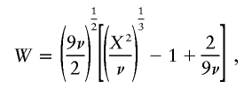
To perform interpopulation comparisons with a standardized metric, we introduced an empirical measure of LD between pairs of multiallelic markers, denoted as “W,” based on a normalized transformation of the standard χ2 statistic. Compared with the frequently used LD measure D′ (Hedrick 1987), of which the distributional properties are unknown, we found, in independent data sets, that W was less sensitive to factors such as sample size and allele numbers and that it provided a better fit than did D′ to the decline of LD with interlocus distance (authors' unpublished data). We developed this measure rather than using the association metric that others introduced for a similar purpose (Collins et al. 2001), since this latter measure (swept radius) is better suited for diallelic markers and requires collapsing of nonassociated alleles to reduce the loci, in a biased way, to diallelic systems. All the genotypic data were used (i.e., haplotypes in males and diplotypes in females). For haplotype data, a statistical χ2 can be derived from a k×l contingency table, where the entry in the ith row and jth column corresponds to the number of Ai Bj haplotypes. χ2 is then defined as the standard contingency table statistic for tests of the null hypothesis of no association between loci A and B, which is distributed under the null hypothesis as χ2 with (k-1)(l-1) df. With genotype data, the haplotype frequencies must be estimated, and we obtained the relevant statistic in the present study by taking the difference between 2× the log likelihood for a fully saturated model (i.e., the assumption of random mating but not linkage equilibrium, with k×l-1 df) and for a model that has the assumption of random mating and linkage equilibrium (with k+l-2 df). With random mating and under the null hypothesis of linkage equilibrium, the difference is distributed as χ2, with (k-1)(l-1) df. The χ2 measures were determined, respectively, using the programs ldmax and haploxt from the GOLD suite (Abecasis and Cookson 2000) with a pooling threshold set at 7%, and their values were summed in a combined χ2. To reduce the dependence of χ2 on the degrees of freedom, it was transformed to an approximate standard normal deviate, W, by
 |
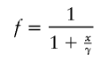
where ν denotes degrees of freedom (Wilson and Hilferty 1931) and where ν=ν1+ν2 (i.e., from haplotypic and diplotypic data). We supposed that the LD measure, W, is related to the genetic-distance measure, x, by the linear form, W=α+βf(x;γ)+ɛ, where α and β are parameters to be estimated, ɛ is a random variable normally distributed with mean 0 and unknown variance σ2, x is the genetic-map distance (in cM), and the link function f is characterized by a single parameter γ, such that f(x=γ;γ)= 1/2, f(x=0;γ)=1, and f(x=∞;γ)=0. Hence, γ can be interpreted as the distance (in cM) at which the expected LD is equal to half the difference between its maximum (α+β, at x=0) and minimum (α, at x=∞) expected values (γ is referred to as the LD–half distance [distance at which LD decays to half the difference between its maximum and minimum value]). This parameter γ provides a measure of the strength of LD. The link function
 |
was fitted. Maximum-likelihood estimates were obtained for α, β, and γ, and the goodness of fit was assessed using the deviance (-2× the log-likelihood ratio), with 2 df (see fig. 3 for illustration of the linear model fitting). Most of the weight is given by the short intermarker distances (<1.5 cM), to which marker pairs on Xq13-11 and Xp21-11 contribute equally but disproportionately compared with the other X-linked markers. The marker pair DXS1225-DXS8082 was removed as being atypical (i.e., in strong LD in all populations examined worldwide). The Scottish subpopulations displayed a 270-fold range of LD–half distances (however, with large associated CIs), from low values in the general U.K. population (0.003 cM) and urban Edinburgh (0.01cM) to increased values in mainland rural subpopulations—Galloway (0.026 cM), Argyll (0.059 cM), Angus (0.14 cM), Borders (0.18 cM), and Grampian (0.21 cM)—and highest levels in the island populations of Shetland (0.22 cM), Orkney (0.29 cM), Wester Ross/Skye (0.29 cM), and Lewis (0.8 cM) (fig. 4). The lower and upper support intervals (which correspond to a 90% CI) for Lewis are 0.5–1.7 cM, compared with 0–0.07 cM for the general U.K. and urban Edinburgh populations, which represents a difference of at least 8-fold. A similar continuum in the extent of LD among the populations studied was obtained when analyzing the subset of male haplotypes (i.e., with no inference bias) on Xq13-21, by use of a different measure of disequilibrium (an exact test) for comparison with published data sets (tables 4 and 5).
Figure 3.

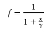 |
Figure 4.

LD decay in 10 Scottish subpopulations and unrelated U.K. subjects, on the basis of 34 X-linked STR markers. Maximum-likelihood estimates of LD–half distance are indicated by a blackened circle. Subpopulations are ordered by increasing values of these estimates. Upper and lower support limits were defined by values of the likelihood equal to 26% of the maximum (equivalent to a 90% CI for estimates with a normally distributed error). The Angus sample size was low (n=78) and had missing data, so that the upper bound for its half-distance decay is high (2.5 cM).
Table 4.
Comparison of Pairwise LD at Xq13-21 for the Male Haplotypes from Our Study and Representative Published Data Sets[Note]
|
Pairwise LD for Male Haplotypes of Subjects from |
||||||||||||||||
| Locus Pair | Distance(cM) | United Kingdom(n=47) | Edinburgh(n=56) | Borders(n=36) | Galloway(N=49) | Angus(n=33) | Argyll(n=30) | Grampian(n=45) | Wester Ross/Skye(n=54) | Orkney(n=51) | Shetland(n=50) | Lewis(n=54) | Finlanda(n=80) | Sardiniab(n=73) | Bozioc(n=51) | Saamia(n=54) |
| DXS8092-DXS8037 | .01 | .697 | .086 | .320 | .460 | .602 | .057 | .522 | .200 |
.034 |
.004 |
.034 |
.180 | .285 | .131 | .000 |
| DXS1225-DXS8082 | .03 | .000 | .000 | .000 | .000 | .000 | .000 | .000 | .000 | .000 | .000 | .000 | .000 | .000 | .000 | .000 |
| DXS8037-DXS1225 | .20 | .644 | .802 | .889 | .916 | .758 | .426 | .121 | .091 | .853 | .009 | .277 | .836 | .710 | .003 | .091 |
| DXS8092-DXS1225 | .21 | .273 | .202 | .330 | .566 | .656 | .445 | .483 | .064 | .161 | .002 | .135 | .283 | .921 | .902 | .000 |
| DXS8037-DXS8082 | .22 | .215 | .812 | .637 | .117 | .563 | .996 | .011 | .003 | .224 | .001 |
.023 |
.238 | .630 | .253 |
.012 |
| DXS8092-DXS8082 | .23 | .936 | .083 | .873 | .487 | .757 | .855 | .053 | .296 | .302 |
.043 |
.206 |
.044 |
.319 | .029 | .000 |
| DXS8082-DXS995 | .61 | .982 | .432 | .730 | .517 | .058 | .798 | .454 | .542 | .815 |
.021 |
.192 | .128 | .430 | .573 | .000 |
| DXS1225-DXS995 | .64 | .650 | .836 | .625 | .322 | .686 | .891 | .925 | .685 | .145 |
.026 |
.017 |
.154 | .355 | .102 | .001 |
| DXS8037-DXS995 | .84 | .736 | .401 | .726 | .301 | .922 | .541 | .512 | .994 | .147 |
.042 |
.034 |
.874 | .650 | .000 | .124 |
| DXS8092-DXS995 | .85 | .485 | .654 | .055 | .320 | .486 |
.030 |
.416 | .503 | .442 | .188 | .713 | .115 | .829 | .019 | .104 |
| DXS983-DXS8092 | 2.51 | .880 | .684 | .648 | .995 | .843 |
.036 |
.446 | .180 | .831 | .641 | .874 | .314 | .876 | .589 | .000 |
| DXS983-DXS8037 | 2.52 | .406 | .789 | .369 | .429 | .494 | .604 | .599 | .442 | .914 | .755 | .456 | .683 |
.036 |
.682 | .300 |
| DXS983-DXS1225 | 2.72 | .270 | .206 | .932 | .164 | .327 | .415 | .047 | .436 | .591 | .184 | .007 | .630 | .169 | .006 | .000 |
| DXS983-DXS8082 | 2.75 | .136 | .987 | .093 | .191 |
.038 |
.436 | .138 | .981 | .796 | .651 | .545 | .565 | .142 | .286 | .000 |
| DXS983-DXS995 | 3.36 | .285 | .391 | .586 | .175 | .086 | .236 | .832 | .979 | .964 | .222 | .008 | .508 | .394 | .090 |
.012 |
Note.— The significance of allelic associations between each possible pair of loci on Xq13-21 typed in male individuals was calculated using Fisher’s exact test, as implemented in Genepop. The Markov-chain parameters were the default values for the number of dememorization steps (1,000) and of iterations per batch (1,000), but the number of batches was adjusted so that the SE of the estimated P value was <.01. Uncorrected P values from Fisher’s exact test were used to classify the table. Values remaining significant at the 5% level, after correction for multiple tests by use of the Holm-Sidak procedure, are shown in bold italics, whereas suggestive P values that are no longer significant after correction are underlined. For Orkney and Shetland, female haplotypes, the phases of which were unambiguously inferred from related individuals otherwise discarded from the study, were used to increase the sample size of male haplotypes and thereby achieve a more homogeneous sample size.
Data reported by Laan and Pääbo (1997).
Data reported by Zavattari et al. (2000).
Data for males from Corsican village reported by Latini et al. (2004).
Table 5.
Pairwise Significance of LD, for All Pairs of STR Loci Studied at Xq13-21 in Male Haplotypes[Note]
|
Pairwise Significance of LD for Male Haplotypes of Subjects from |
||||||||||||
| Locus Pair | Distance (cM) | United Kingdom(n=47) | Edinburgh(n=56) | Borders(n=36) | Galloway(n=49) | Angus(n=33) | Argyll(n=30) | Grampian(n=45) | Wester Ross/Skye(n=54) | Orkney(n=51) | Shetland(n=50) | Lewis(n=54) |
| DXS8092-DXS8037 | .01 | .697 | .086 | .320 | .460 | .602 | .057 | .522 | .200 |
.034 |
.004 |
.034 |
| DXS1225-DXS8082 | .03 | .000 | .000 | .000 | .000 | .000 | .000 | .000 | .000 | .000 | .000 | .000 |
| DXS56-DXS1225 | .06 | .685 | .395 | .297 | .015 | .322 | .250 |
.048 |
.002 | .293 |
.021 |
.005 |
| DXS56-DXS8082 | .09 | .713 | .562 | .477 | .732 | .140 | .742 | .061 | .007 | .429 | .147 | .000 |
| DXS8037-DXS56 | .13 | .910 | .414 | .006 | .935 | .174 | .046 | .010 | .019 | .000 | .000 |
.011 |
| DXS8092-DXS56 | .14 |
.042 |
.584 | .166 | .707 | .120 | .439 | .025 | .207 | .003 | .002 | .222 |
| DXS8037-DXS1225 | .20 | .644 | .802 | .889 | .916 | .758 | .426 | .121 | .091 | .853 | .009 | .277 |
| DXS8092-DXS1225 | .21 | .273 | .202 | .330 | .566 | .656 | .445 | .483 | .064 | .161 | .002 | .135 |
| DXS8037-DXS8082 | .22 | .215 | .812 | .637 | .117 | .563 | .996 | .011 | .003 | .224 | .001 |
.023 |
| DXS8092-DXS8082 | .23 | .936 | .083 | .873 | .487 | .757 | .855 | .053 | .296 | .302 |
.043 |
.206 |
| DXS8082-DXS995 | .61 | .982 | .432 | .730 | .517 | .058 | .798 | .454 | .542 | .815 |
.021 |
.192 |
| DXS1225-DXS995 | .64 | .650 | .836 | .625 | .322 | .686 | .891 | .925 | .685 | .145 |
.026 |
.017 |
| DXS56-DXS995 | .70 | .630 | .142 | .178 | .415 | .595 | .470 | .763 | .313 | .070 | .810 | .008 |
| DXS8037-DXS995 | .84 | .736 | .401 | .726 | .301 | .922 | .541 | .512 | .994 | .147 |
.042 |
.034 |
| DXS8092-DXS995 | .85 | .485 | .654 | .055 | .320 | .486 |
.030 |
.416 | .503 | .442 | .188 | .713 |
| DXS1165-DXS8092 | .98 | .596 | .772 | .278 | .727 | .815 | .067 | .921 | .001 |
.026 |
.041 |
.025 |
| DXS1165-DXS8037 | 1.00 | .612 | .856 | .079 | .090 | .003 |
.037 |
.069 | .541 | .416 | .003 |
.021 |
| DXS1165-DXS56 | 1.13 | .434 | .898 | .412 | .514 | .522 | .248 | .533 | .573 | .185 | .624 | .128 |
| DXS1165-DXS1225 | 1.19 | .172 | .282 | .397 | .382 | .017 | .056 | .355 | .260 | .054 | .052 | .001 |
| DXS1165-DXS8082 | 1.22 | .382 | .067 | .224 |
.039 |
.289 | .608 | .082 | .395 | .008 | .001 | .000 |
| DXS983-DXS1165 | 1.53 | .169 | .525 | .623 | .263 | .871 | .843 | .557 | .307 | .769 | .216 | .391 |
| DXS1165-DXS995 | 1.83 | .514 | .924 | .760 |
.031 |
.581 | .255 | .482 | .177 | .374 | .354 | .762 |
| DXS983-DXS8092 | 2.51 | .880 | .684 | .648 | .995 | .843 |
.036 |
.446 | .180 | .831 | .641 | .874 |
| DXS983-DXS8037 | 2.52 | .406 | .789 | .369 | .429 | .494 | .604 | .599 | .442 | .914 | .755 | .456 |
| DXS983-DXS56 | 2.66 | .860 | .377 | .282 | .105 | .483 | .983 | .317 | .655 | .094 | .745 | .440 |
| DXS983-DXS1225 | 2.72 | .270 | .206 | .932 | .164 | .327 | .415 | .047 | .436 | .591 | .184 | .007 |
| DXS983-DXS8082 | 2.75 | .136 | .987 | .093 | .191 |
.038 |
.436 | .138 | .981 | .796 | .651 | .545 |
| DXS983-DXS995 | 3.36 | .285 | .391 | .586 | .175 | .086 | .236 | .832 | .979 | .964 | .222 |
.008 |
Note.— Values remaining significant at the 5% level, after correction for multiple tests by use of the Holm-Sidak procedure, are shown in bold italics, whereas suggestive P values, no longer significant after correction, are underlined.
To evaluate the effect of sampling between rather than within subpopulations on the extent of LD, 15 randomized samples of size 100 were created by bootstrap sampling across mainland rural areas, in accordance with their census size. The average LD–half distance obtained was 0.089 cM (90% CI 0.061–0.129), which indicates reduced LD compared with four of the rural subpopulations taken singly (0.14, 0.18, 0.21, and 0.29 cM). Similarly, sampling within all of mainland Scotland, including the urban center of Edinburgh, a scheme similar to the U.K. Biobank design, led to an even smaller LD–half distance of 0.062cM (90% CI 0.044–0.088).
These conclusions are based on the analysis of STR markers that span only two regions of the X chromosome—for which LD extent has been shown to be generally greater than for autosomes (Taillon-Miller et al. 2004)—as expected, since their effective population size is three-quarters that of the autosomes. The LD–half distance is thus likely to be scaled down for autosomal STRs, and more so for SNPs, which have lower mutation rates, so that the detection of differences between populations with SNPs would require considerably more markers to be typed. The X-linked STR markers therefore provide sensitive measures of differentiation with efficient detection and quantification of population differences arising from demographic and other factors. Demographic factors act globally across the genome, whereas local factors such as recombination rates and selection may be region specific. There is no evidence, to date, that these two investigated chromosomal regions have been subject to significant selection. In two previous studies, these X-chromosome regions displayed extended LD in isolated populations compared with nonisolate populations, which was also observed in autosomal regions (Zavattari et al. 2000; Kaessmann et al. 2002). Critically, the power to detect association declines exponentially rather than linearly as the extent of LD falls toward zero (Blangero 2004), which suggests that even a small increase in the extent of LD could increase power and reduce cost by more than an order of magnitude.
Genetic Complexity
The extent of LD between marker loci reflects the amount of historical recombination and past effective population size (Ne), so that, for a given genomic region, LD can differ dramatically between populations with different demographic histories (Pritchard and Przeworski 2001). We aimed to explore the level of LD between X-chromosomal STRs in relation to the predicted effective population size, Ne. Ne reflects the number of ancestors who have contributed to the gene pool. The more Ne is reduced, the greater the effect of genetic drift and the greater the genealogical relationship within a sample, which, in turn, can result in increased LD. Therefore, for Xp21-11 and Xq13-21, female haplotypes were inferred using the Bayesian statistical method implemented in PHASE (v2.0.2) on the basis of the coalescent model (Stephens et al. 2001). The algorithm that integrates recombination in the simulations (Li and Stephens 2003) was run independently five times, and the run with the best average goodness of fit to the approximate coalescent model was kept. Point estimates of the population average recombination parameter 3Ner were obtained by taking the median value among 1,000 sampled from the corresponding posterior distribution, as implemented in PHASE (v2.0.2). The values shown in table 6 display a ranking similar to that obtained for the extent of LD, which is especially clear for the more recombinogenic chromosomal region (i.e., Xp21-11) data, from high values in the urban and U.K. samples to intermediate values in the Scottish mainland regions to low values in the islands. The differences between subpopulations, within each chromosomal region, can be attributed to differences in effective population size (Ne). Although the posterior distributions of the recombination parameters overlap, there is a clear trend toward a reduction in Ne in Orkney, Lewis, Shetland, and Wester Ross/Skye compared with U.K. or Edinburgh (in the range of 2–5-fold), which implies a less complex gene pool (table 6). This was noticeable by the reduction in computation time when running the PHASE-implemented algorithm for the island subpopulations. Within each subpopulation, the estimates obtained in the two investigated chromosomal regions were significantly correlated (Spearman’s rank correlation 63%; P=.02), and the difference between Xq13-21 and Xp21-11 average recombination estimates are in agreement with pedigree-based estimates (6-fold [Kong et al. 2002]), suggesting that the coalescence-based algorithm performed well.
Table 6.
Median Population Recombination-Rate Estimates[Note]
|
3Ner (Ne) for Loci on |
||
| Population | Xp21-11a | Xq13-21b |
| Shetland | 21×10−6 (1,400) | 3.4×10⁻⁶ (435) |
| Lewis | 21×10−6 (1,400) | 6.1×10⁻⁶ (782) |
| Orkney | 44×10−6 (2,933) | 8.7×10⁻⁶ (1,115) |
| Galloway | 44×10−6 (2,933) | 15.8×10⁻⁶ (2,025) |
| Wester Ross/Skye | 46×10−6 (3,067) | 6.5×10⁻⁶ (833) |
| Argyll | 46×10−6 (3,067) | 7.5×10⁻⁶ (961) |
| Grampian | 60×10−6 (4,000) | 14.3×10⁻⁶ (1,833) |
| Angus | 77×10−6 (5,133) | 18.0×10⁻⁶ (2,031) |
| United Kingdom | 94×10−6 (6,267) | 11.7×10⁻⁶ (1,500) |
| Edinburgh | 94×10−6 (6,267) | 29.0×10⁻⁶ (3,718) |
| Borders | 100×10−6 (6,667) | 14.1×10⁻⁶ (1,808) |
Note.— Subpopulations are shown in increasing order, by values of their adjusted recombination rate based on Xp21-11 data. Estimates of the population-adjusted recombination rates, 3Ner, were obtained after haplotype inference from female genotypes by use of the coalescent model implemented in PHASE v2.0.2. The algorithm was run independently five times, and the run with the best average goodness of fit to the approximate coalescent model was kept. Within each run, the number of iterations of the final step (i.e., all loci considered) was increased by a factor of 10, compared with the default setting, to obtain better estimates. The median of 1,000 values sampled from the posterior distribution was taken as point estimate for each population-adjusted recombination rate. The units of r are per meiosis and per base pair.
Within Xp21-11, 13 Xp11 markers (DXS1068, DXS8014, DXS8113, DXS1058, DXS8015, DXS8042, DXS1368, DXS993, DXS8012, DXS1201, DXS8085, DXS7, and MAOB), spanning 4.7 Mb (7 cM), were used.
Within Xq13-21, all eight markers (DXS983, DXS1165, DXS8092, DXS8037, DXS56, DXS1225, DXS8082, and DXS995) were used, spanning 13 Mb (3.36 cM). Estimates of the subpopulation effective size were calculated from the average map-based estimate of recombination rates.
The observed increase in LD seen in rural subpopulations is also mirrored by the haplotype-diversity data. Table 7 shows haplotypes for six STRs on Xq13-21 that span 0.85 cM, together with a subset of three STR haplotypes. For six-locus haplotypes, the highest haplotype diversity was found in Edinburgh (98% of haplotypes were different) and the U.K. (96%), and the lowest diversity was found in Orkney (76%), Shetland (76%), and Lewis (64%). Gene diversity, a measure based on allele frequency, was estimated for Xq13-21 markers and was very similar across regions, although it tended to be lower for the Lewis subpopulation (table 7).
Table 7.
Gene and Haplotype Diversity of a Subset of Six Xq13-21 Markers[Note]
|
Findings for Haplotype Set |
||||||||||||
|
DXS8092-DXS8037-DXS56-DXS1225-DXS8082-DXS995 |
DXS56-DXS1225-DXS8082 |
Gene diversity (No. of Alleles) for Haplotypeb |
||||||||||
| Populationa | Nc | kd (%) | Nc | kd (%) | DXS983 | DXS1165 | DXS8092 | DXS8037 | DXS56 | DXS1225 | DXS8082 | DXS995 |
| Lewis | 101 | 65 (64) | 169 | 37 (22) | .64 (5) | .67 (8) | .83 (11) | .68 (10) | .74 (10) | .74 (11) | .73 (10) | .57 (5) |
| Shetland | 58 | 44 (76) | 87 | 32 (37) | .62 (6) | .67 (10) | .85 (11) | .71 (7) | .76 (8) | .74 (10) | .74 (8) | .61 (6) |
| Orkney | 73 | 56 (76) | 99 | 38 (38) | .63 (9) | .68 (10) | .85 (13) | .69 (8) | .79 (10) | .73 (12) | .71 (9) | .59 (5) |
| Argyll | 58 | 48 (83) | 102 | 42 (41) | .59 (5) | .66 (10) | .84 (11) | .68 (8) | .77 (8) | .75 (10) | .77 (9) | .67 (5) |
| Grampian | 49 | 41 (84) | 72 | 36 (50) | .66 (6) | .68 (9) | .86 (13) | .71 (8) | .78 (9) | .76 (11) | .68 (9) | .52 (7) |
| Wester Ross/Skye | 61 | 53 (87) | 97 | 40 (41) | .64 (5) | .68 (9) | .85 (12) | .73 (9) | .74 (9) | .74 (11) | .73 (9) | .63 (6) |
| Borders | 46 | 42 (91) | 90 | 37 (41) | .65 (8) | .73 (6) | .86 (12) | .73 (10) | .75 (8) | .76 (11) | .76 (9) | .57 (6) |
| Galloway | 56 | 51 (91) | 94 | 47 (50) | .69 (7) | .67 (11) | .88 (12) | .66 (8) | .80 (8) | .75 (10) | .78 (10) | .61 (5) |
| Angus | 34 | 32 (94) | 56 | 25 (45) | .69 (6) | .69 (9) | .87 (14) | .68 (7) | .79 (8) | .74 (11) | .74 (9) | .66 (6) |
| United Kingdom | 53 | 51 (96) | 101 | 46 (46) | .70 (7) | .67 (11) | .87 (13) | .66 (9) | .78 (8) | .77 (11) | .75 (10) | .59 (6) |
| Edinburgh | 40 | 39 (97.5) | 87 | 40 (57) | .68 (8) | .74 (11) | .86 (14) | .70 (10) | .79 (8) | .76 (12) | .77 (10) | .54 (6) |
Note.— Allele frequencies for each microsatellite locus were estimated using Genepop software. Nei’s average heterozygosity, or gene diversity, was calculated as 1 − the sum of the squared allele frequencies.
Subpopulations are shown in increasing order, by values of the six-loci haplotype diversity.
Gene diversity is based on whole data set.
N = number of complete (i.e., without missing data) Xq13-21 six- or three-locus haplotypes from the male data set and inferred from the female data set. (For the inferred haplotype at each locus, the genotypes with phase certainty under 80% were discarded.)
k = number of distinct haplotypes.
Discussion
The Scottish island populations represent both unusually stable and older populations whose declining numbers—due to past bottlenecks, large-scale emigration, and little immigration—may have contributed to the creation of LD as a result of genetic drift and endogamous mating. Clear evidence of a reduced female gene pool had been reported in the Western Isles and Orkney, on the basis of the low mtDNA diversity in the region (Helgason et al. 2001). These populations may be suitable for the drift-mapping strategy (Terwilliger et al. 1998), as proposed for mapping genetic factors that influence complex disease. In our study, the island of Lewis appeared to be the most extreme with regard to the extent of LD, in agreement with a previous report showing high differentiation, compared with Ireland and mainland Scotland, on the basis of serum protein polymorphisms (Clegg et al. 1985).
Interestingly, despite little differentiation based on allele-frequency distributions, evidence for population structure was also detectable in mainland rural subpopulations (e.g., Galloway, Grampian, and Argyll), which showed levels of LD intermediate between the urban/general U.K. and island samples. This intermediate extent of LD is likely to reflect increased sharing of ancestral chromosomal segments. Because of their larger size compared with that of the islands (fig. 1), these subpopulations (91,000–314,000) represent a valuable resource for conducting large-scale genetic-association studies, especially when a high percentage of the population is “local”—such as in Grampian (42% local), which is comparable in population size to Iceland. Variable levels of LD among populations that are not differentiated by allele-frequency distributions have been observed in at least one other study. Although differentiation, as estimated by pairwise FST, was not significant between the Saami and the Finnish populations when SNP data from ACE, β-globin, LPL, and MX were combined, these populations showed very different levels of LD (Kaessmann et al. 2002). The extent of LD appears to be more sensitive to factors such as reduction in effective population size and/or levels of endogamy than to measures of differentiation based on allele-frequency distributions (e.g., FST).
Finally, it is clear that the advantages of sampling within rural subpopulations, such as for reduced haplotype diversity and increased extent of LD for association mapping, are diminished by sampling across multiple regions or from within large urban populations. An increasing number of national genetic databases are being set up to exploit the biomedical opportunities offered by dense, high-throughput SNP genotyping in the context of association studies. The U.K. Biobank study is the largest of such studies to date, which proposes recruitment of 500,000 individuals from across the United Kingdom, including 80,000 from Scotland. Recruitment strategies for such large-scale studies tend to be representative of the population as a whole and therefore underrepresent rural populations. The higher haplotype diversity and low levels of LD within urban samples may make whole-genome scans prohibitively expensive and either increase the cost or reduce the power of more-focused genotyping studies. The major value of such national collections may therefore be not in the discovery of new genetic associations but in the further characterization of known ones. There is a strong case for additional biobanks of individuals recruited from large, stable rural subpopulations, which have the potential for providing increased power and efficiency to detect new genetic variants influencing biomedical traits.
Acknowledgments
The authors are indebted to the participants who allowed use of their DNA for this study and to the general practitioners who agreed to take part in the study. We thank Yoshiro Shibasaki, for help in making early contacts; Pauline McDonald and Lindsey Walls, for their secretarial help in the recruitment phase; Susan Fitzsimmon and Isla Campbell, for help in genotyping; and Douglas Stuart, for figure reproduction. This research received support from the U.K. Medical Research Council (MRC). V.V. holds an MRC Special Training Fellowship in Bioinformatics.
Electronic-Database Information
The URLs for data presented herein are as follows:
- Authors' Web site, http://www.hgu.mrc.ac.uk/Rawdata/AJHG76/Vitart/ (for the authors' raw data)
- Genepop, http://wbiomed.curtin.edu.au/genepop/
- Genetix, http://www.univ-montp2.fr/~genetix/genetix/genetix.htm
- GOLD, http://www.well.ox.ac.uk/asthma/GOLD/
- PHASE, http://www.stat.washington.edu/stephens/software.html
References
- Abecasis GR, Cookson WO (2000) GOLD—graphical overview of linkage disequilibrium. Bioinformatics 16:182–183 10.1093/bioinformatics/16.2.182 [DOI] [PubMed] [Google Scholar]
- Angius A, Bebbere D, Petretto E, Falchi M, Forabosco P, Maestrale B, Casu G, Persico I, Melis PM, Pirastu M (2002) Not all isolates are equal: linkage disequilibrium analysis on Xq13.3 reveals different patterns in Sardinian sub-populations. Hum Genet 111:9–15 10.1007/s00439-002-0753-z [DOI] [PubMed] [Google Scholar]
- Blangero J (2004) Localization and identification of human quantitative trait loci: king harvest has surely come. Curr Op Genet Dev 14:233–240 10.1016/j.gde.2004.04.009 [DOI] [PubMed] [Google Scholar]
- Brown ES (1965) Distribution of ABO and Rhesus (D) blood groups in the North of Scotland. Heredity 20:289–303 [DOI] [PubMed] [Google Scholar]
- Capelli C, Redhead N, Abernethy JK, Gratrix F, Wilson JF, Moen T, Hervig T, Richards M, Stumpf MP, Underhill PA, Bradshaw P, Shaha A, Thomas MG, Bradman N, Goldstein DB (2003) A Y chromosome census of the British Isles. Curr Biol 13:979–984 10.1016/S0960-9822(03)00373-7 [DOI] [PubMed] [Google Scholar]
- Clegg EJ, Tills D, Warlow A, Wilkinson J, Marin A (1985) Blood group variation in the Isle of Lewis. Ann Hum Biol 12:345–361 [DOI] [PubMed] [Google Scholar]
- Collins A, Ennis S, Taillon-Miller P, Kwok PY, Morton NE (2001) Allelic association with SNPs: metrics, populations, and the linkage disequilibrium map. Hum Mutat 17:255–262 10.1002/humu.21 [DOI] [PubMed] [Google Scholar]
- Freedman ML, Reich D, Penney KL, McDonald GJ, Mignault AA, Patterson N, Gabriel SB, Topol EJ, Smoller JW, Pato CN, Pato MT, Petryshen TL, Kolonel LN, Lander ES, Sklar P, Henderson B, Hirschhorn JN, Altshuler D (2004) Assessing the impact of population stratification on genetic association studies. Nat Genet 36:388–393 10.1038/ng1333 [DOI] [PubMed] [Google Scholar]
- Hedrick PW (1987) Gametic disequilibrium measures: proceed with caution. Genetics 117:331–341 [DOI] [PMC free article] [PubMed] [Google Scholar]
- Helgason A, Hickey E, Goodacre S, Bosnes V, Stefánsson K, Ward R, Sykes B (2001) mtDNA and the islands of the North Atlantic: estimating the proportions of Norse and Gaelic ancestry. Am J Hum Genet 68:723–737 [DOI] [PMC free article] [PubMed] [Google Scholar]
- Helgason A, Sigurðardóttir S, Nicholson J, Sykes B, Hill EW, Bradley DG, Bosnes V, Gulcher JR, Ward R, Stefánsson K (2000) Estimating Scandinavian and Gaelic ancestry in the male settlers of Iceland. Am J Hum Genet 67:697–717 [DOI] [PMC free article] [PubMed] [Google Scholar]
- Helgason A, Yngvadottir B, Hrafnkelsson B, Gulcher J, Stefánsson K (2005) An Icelandic example of the impact of population structure on association studies. Nat Genet 37:90–95 [DOI] [PubMed] [Google Scholar]
- Kaessmann H, Zöllner S, Gustafsson AC, Wiebe V, Laan M, Lundeberg J, Uhlén M, Pääbo S (2002) Extensive linkage disequilibrium in small human populations in Eurasia. Am J Hum Genet 70:673–685 [DOI] [PMC free article] [PubMed] [Google Scholar]
- Katoh T, Mano S, Ikuta T, Munkhbat B, Tounai K, Ando H, Munkhtuvshin N, Imanishi T, Inoko H, Tamiya G (2002) Genetic isolates in East Asia: a study of linkage disequilibrium in the X chromosome. Am J Hum Genet 71:395–400 [DOI] [PMC free article] [PubMed] [Google Scholar]
- Kong A, Gudbjartsson DF, Sainz J, Jonsdottir GM, Gudjonsson SA, Richardsson B, Sigurdardottir S, Barnard J, Hallbeck B, Masson G, Shlien A, Palsson ST, Frigge ML, Thorgeirsson TE, Gulcher JR, Stefansson K (2002) A high-resolution recombination map of the human genome. Nat Genet 31:241–247 [DOI] [PubMed] [Google Scholar]
- Kruskal JB, Wish M (1977) Multidimensional scaling. Sage Publications, Beverly Hills [Google Scholar]
- Laan M, Pääbo S (1997) Demographic history and linkage disequilibrium in human populations. Nat Genet 17:435–438 10.1038/ng1297-435 [DOI] [PubMed] [Google Scholar]
- Latini V, Sole G, Doratiotto S, Poddie D, Memmi M, Varesi L, Vona G, Cao A, Ristaldi MS (2004) Genetic isolates in Corsica (France): linkage disequilibrium extension analysis on the Xq13 region. Eur J Hum Genet 12:613–619 10.1038/sj.ejhg.5201205 [DOI] [PubMed] [Google Scholar]
- Li N, Stephens M (2003) Modeling linkage disequilibrium and identifying recombination hotspots using single-nucleotide polymorphism data. Genetics 165:2213–2233 [DOI] [PMC free article] [PubMed] [Google Scholar]
- Marchini J, Cardon LR, Phillips MS, Donnelly P (2004) The effects of human population structure on large genetic association studies. Nat Genet 36:512–517 10.1038/ng1337 [DOI] [PubMed] [Google Scholar]
- Mourant AE, Kopéc AC, Domaniewska-Sobczak K (1976) The distribution of the human blood groups and other polymorphisms. Oxford University Press, London [Google Scholar]
- Nei M (1978) Estimation of average heterozygosity and genetic distance from a small number of individuals. Genetics 89:583–590 [DOI] [PMC free article] [PubMed] [Google Scholar]
- Pritchard JK, Przeworski M (2001) Linkage disequilibrium in humans: models and data. Am J Hum Genet 69:1–14 [DOI] [PMC free article] [PubMed] [Google Scholar]
- Pritchard JK, Stephens M, Donnelly P (2000) Inference of population structure using multilocus genotype data. Genetics 155:945–959 [DOI] [PMC free article] [PubMed] [Google Scholar]
- Raymond M, Rousset F (1995) An exact test for population differentiation. Evolution 49:1280–1283 [DOI] [PubMed] [Google Scholar]
- Stephens M, Smith NJ, Donnelly P (2001) A new statistical method for haplotype reconstruction from population data. Am J Hum Genet 68:978–989 [DOI] [PMC free article] [PubMed] [Google Scholar]
- Taillon-Miller P, Saccone SF, Saccone NL, Duan S, Kloss EF, Lovins EG, Donaldson R, Phong A, Ha C, Flagstad L, Miller S, Drendel A, Lind D, Miller RD, Rice JP, Kwok PY (2004) Linkage disequilibrium maps constructed with common SNPs are useful for first-pass disease association screens. Genomics 84:899–912 10.1016/j.ygeno.2004.08.009 [DOI] [PubMed] [Google Scholar]
- Terwilliger JD, Zollner S, Laan M, Paabo S (1998) Mapping genes through the use of linkage disequilibrium generated by genetic drift: “drift mapping” in small populations with no demographic expansion. Hum Heredity 48:138–154 10.1159/000022794 [DOI] [PubMed] [Google Scholar]
- Weir BS, Cockerham CC (1984) Estimating F-statistics for the analysis of population structure. Evolution 38:1358–1370 [DOI] [PubMed] [Google Scholar]
- Wilson EB, Hilferty MM (1931) The distribution of chi-square. Proc Natl Acad Sci USA 17:694 [DOI] [PMC free article] [PubMed] [Google Scholar]
- Wilson JF, Weiss DA, Richards M, Thomas MG, Bradman N, Goldstein DB (2001) Genetic evidence for different male and female roles during cultural transitions in the British Isles. Proc Natl Acad Sci USA 98:5078–5083 10.1073/pnas.071036898 [DOI] [PMC free article] [PubMed] [Google Scholar]
- Zavattari P, Deidda E, Whalen M, Lampis R, Mulargia A, Loddo M, Eaves I, Mastio G, Todd JA, Cucca F (2000) Major factors influencing linkage disequilibrium by analysis of different chromosome regions in distinct populations: demography, chromosome recombination frequency and selection. Hum Mol Genet 9:2947–2957 10.1093/hmg/9.20.2947 [DOI] [PubMed] [Google Scholar]