Nonparametric Tests of Association of Multiple Genes with Human Disease

Abstract

The genetic basis of many common human diseases is expected to be highly heterogeneous, with multiple causative loci and multiple alleles at some of the causative loci. Analyzing the association of disease with one genetic marker at a time can have weak power, because of relatively small genetic effects and the need to correct for multiple testing. Testing the simultaneous effects of multiple markers by multivariate statistics might improve power, but they too will not be very powerful when there are many markers, because of the many degrees of freedom. To overcome some of the limitations of current statistical methods for case-control studies of candidate genes, we develop a new class of nonparametric statistics that can simultaneously test the association of multiple markers with disease, with only a single degree of freedom. Our approach, which is based on U-statistics, first measures a score over all markers for pairs of subjects and then compares the averages of these scores between cases and controls. Genetic scoring for a pair of subjects is measured by a “kernel” function, which we allow to be fairly general. However, we provide guidelines on how to choose a kernel for different types of genetic effects. Our global statistic has the advantage of having only one degree of freedom and achieves its greatest power advantage when the contrasts of average genotype scores between cases and controls are in the same direction across multiple markers. Simulations illustrate that our proposed methods have the anticipated type I–error rate and that they can be more powerful than standard methods. Application of our methods to a study of candidate genes for prostate cancer illustrates their potential merits, and offers guidelines for interpretation.

Introduction

The genetic basis of common human diseases is widely studied by evaluating the association of genetic variants with disease status, as in candidate-gene case-control studies. The power of this approach depends on the effect size of the disease locus (typically considered in terms of an odds ratio), the frequency of the disease allele(s), the frequency of the marker allele(s), and the magnitude of linkage disequilibrium between the marker and disease loci (Zondervan and Cardon 2004). Although there is debate on whether common diseases are caused by many rare mutations (Pritchard and Cox 2002) or a few common genetic variants (Reich and Lander 2001), it is clear that allelic heterogeneity will dilute power to detect genetic associations (Slager et al. 2000). Furthermore, when multiple genes are functionally related—for instance, when their products are related through a cascade of enzymatic reactions—mutations at any of several genes could lead to disease. Also, it may not be unusual for genes in a functional pathway to have complex interactions, given evidence of feedback loops and compensatory enzymatic activities among the protein products of biosynthesis pathways.

Standard methods to evaluate the association of multiple markers with disease status are based on either single-marker analyses or multimarker multivariate analyses. For single-marker analyses of diallelic markers, it is common to compare the allele frequencies of each marker between cases and controls by use of Armitage’s test for trend (Sasieni 1997) and to adjust for multiple testing by use of either the Bonferroni correction or a permutation P value for the most extreme statistic. This approach is likely to be most powerful if there is only a single marker strongly associated with disease. For multimarker multivariate analyses, one can use logistic regression to test simultaneously the main effects (and possibly interactions) of multiple markers. For each marker, a covariate can be created, such as the number of rare alleles at each marker. When this type of coding is used in logistic regression, the resulting score statistic for each marker is Armitage’s test for trend, so simultaneously testing multiple marker loci by this type of coding and using the score statistic from logistic regression is a multivariate version of Armitage’s score statistic. For K markers, each coded into covariates, the resulting score statistic has a χ² distribution with K degrees of freedom. This statistic is equivalent to the multivariate Hotelling’s T² statistic proposed by Fan and Knapp (2003). Although this approach can be more powerful than testing each marker separately (Longmate 2001), it still suffers from weak power because of the large number of degrees of freedom. When evaluating the association of multiple genes with disease status, the power to detect associations can be weak when the effects of individual genes are weak and when correcting for multiple testing.

An alternative approach to evaluate the association of multiple genes with disease status might be to model all the complex interrelationships of genes, say within a common pathway, and how they relate to disease. This parametric method, however, would lead to models with too many parameters, possibly causing multicollinearity and model instability. Although Bayesian modeling of metabolic pathways with case-control data has achieved some level of success (Conti et al. 2003), it is difficult to evaluate whether complex models are overfitted to the data.

To improve power over that of standard methods, we propose a class of nonparametric statistics that combines information across all genetic markers, resulting in a global statistic that has a standard normal distribution. We expect that this approach would be sensitive to situations in which multiple genes influence the disease but the effect of each individual gene is weak. Our nonparametric methods are based on U-statistics, which are used to measure an average genetic score between pairs of subjects. Intuitively, we expect that any two subjects with similar disease status should also have similar genetic scores if any of the markers are associated with the disease. Hence, we measure the average genetic score for all pairs of cases and compare this to the average genetic score for all pairs of controls.

In the “Statistical Methods” section below, we describe the intuition and derivation of our methods, showing their generality, as well as important special cases. We illustrate how power can be computed, and we use this to show how to determine an optimal genotype score. To illustrate the properties of our methods, we perform simulations. We also apply our methods to a study of candidate genes for prostate cancer, to illustrate their utility and interpretation.

Statistical Methods

To compare the distribution of all marker genotypes between cases and controls, we first compute the scores for all possible pairs of subjects within each of the case and control groups. We then contrast the average scores between cases and controls by use of a global statistic with one degree of freedom instead of the implicit many degrees of freedom when many markers are analyzed.

U-Statistics for Within-Group Genotype Scores

First, consider a measure of genotype score within a single group of n subjects. Let g_i denote a vector of measured genotypes at K markers for subject i, with element g_i,k the kth genotype. To measure the score of all genotypes for subjects i and j, we use a symmetric kernel, denoted as h(g_i,g_j). A general U-statistic that measures the average score across all pairs of subjects is

Hence, no matter how many markers are measured, the global U-statistic uses a kernel function to reduce the arrays of genetic markers for pairs of subjects into a single score, which then are averaged across all possible pairs. Although a wide variety of kernels can be considered, we shall consider primarily kernels that are additive across all K markers, so that . In general, the kernel can differ across markers, which might be desirable if we knew that some markers are likely to have dominant effects and others recessive effects. However, we assume that the same kernel is used for all markers, to simplify our presentation. Additive kernels are attractive because they make it easy to account for missing genotypes, weighted sums can be created, and they can be computed rapidly. For example, a weighted sum kernel in equation (1) results in

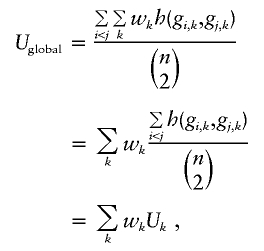emphasizing that U_global is a weighted sum of marker-specific U-statistics. Let U denote the vector of marker-specific U-statistics. We shall contrast the vector U between cases and controls and average this contrast across all markers. First, however, we need to consider the variance matrix for the vector U, because this variance matrix will be used to create optimal weights for averaging across the markers.

We assume that subjects are independent of each other, but genetic markers can be correlated due to linkage disequilibrium, or perhaps natural selection. To determine the asymptotic covariance matrix of U, we use standard results on U-statistics (Hoeffding 1948, Serfling 1980). For now assume that there is no missing data. Let h₁(g_i,k)=E[h(g_i,k,G_j,k)], where lowercase g is fixed and uppercase G is random. In other words, one of the random genotypes is integrated out of the bivariate kernel h to create the marginal function h₁. Then, the asymptotic covariances can be expressed as

where σ_k,l=Cov[h₁(G_i,k),h₁(G_i,l)]. To apply this general expression, we need to account for missing data (i.e., to allow n to vary over the different markers), and we need a way to determine σ_k,l for a specified kernel.

We shall first illustrate the derivation of , where n_k denotes the number of subjects without missing data for marker k. To determine σ_k,k=Var[h₁(G_i,k)], let P(g_k) denote the probability of genotype g_k. The term h₁(g_i,k) can then be expressed as

By using the genotype probabilities again, the expected value of h₁(G_i,k) can be easily derived according to

and its variance according to

Then, .

Now consider . This covariance depends on the number of subjects that contribute to both U_k and U_l; let n_k,l be this number. Then, allowing for missing data,

Note that this expression reduces to expression (2) when there is no missing data (e.g., n_k=n_l=n_k,l). To determine σ_k,l , we reduce the sample to those n_k,l subjects with complete data for both markers, and compute the expected value of h₁(G_i,k)h₁(G_i,l),

where P(g_k,g_l) is the joint probability of genotypes at both markers. This is then used to compute

Computational Issues

The computations of the U_k statistics and their covariances are very time-consuming when summing over all pairs of subjects. The most efficient computational method is to weight the kernel scores by the counts of distinguishable genotypes. Let x_s denote the number of subjects with the sth genotype category (s=1,…,S). Then, U_k can be expressed as

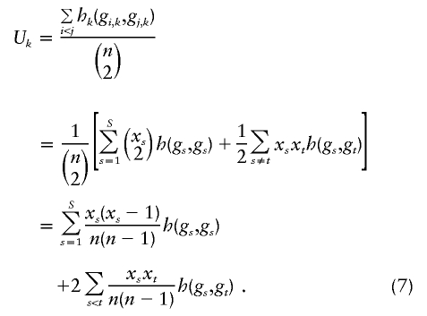The term  1/2 in equation (7) is needed because the sum over s≠t gives a double count. Derivations of other types of U-statistics for genetic studies have emphasized this way of computing U-statistics (Kowalski 2001; Kowalski et al. 2002; Tzeng et al. 2003a, 2003b), and in fact often rely on U=P^′HP+O(1/n), where P is the vector of relative frequencies of the categories (genotypes, in our situation) and H is a symmetric matrix of corresponding kernel scores (Tzeng 2003).

To compute , we use the estimate to compute μ_k (eq. 3) and σ_k,k (eq. 4). To compute , we subset to those subjects not missing data at both markers, create a contingency table of genotype counts for g_k×g_l, with cell counts x_gk,gl, and use estimate in equation (5) to compute σ_k,l.

Contrast of Case with Control Genotype Scores

To compare the vector of within-group scores for cases with that for controls, we use the contrast vector

where the subscripts d and c denote the diseased cases and controls, respectively. Under the null hypothesis of no differences between cases and controls, standard results for U-statistics imply that δ has a multivariate normal distribution with mean zero and covariance matrix V_o, which has elements

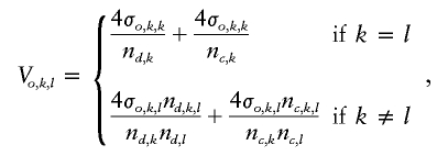where σ_o,k,l is computed under the null hypothesis. This is accomplished by pooling cases and controls to compute estimates and and then using these to estimate σ_o,k,l, as described above in the “Computational Issues” section.

To construct a statistic that is sensitive to alternatives for which all elements of δ are in the same direction (i.e., all positive or all negative), we use a weighted sum of the elements of δ. To choose the weight vector w, we use the generalized least squares procedure, which provides the best (i.e., smallest variance) linear unbiased estimator (BLUE) and corresponding optimal test statistic. In this case, the weight w_k is proportional to the kth row total of V^-1_o. That is,

where 1 is a vector of ones. Hence, the global statistic is

and Z_global has an asymptotic standard normal distribution.

Choice of Kernel for Genotype Scores

A challenging aspect of our proposed methods is the choice of a kernel that is powerful for a wide range of genetic effects. An intuitive choice is to simply count the number of alleles that match between a pair of subjects; we call this the “allele-match” kernel. This type of similarity measure has been used for linkage statistics, such as the affected-pedigree member linkage statistic (Weeks and Lange 1988), and to evaluate the association of haplotypes with disease (Tzeng et al. 2003b). This similarity kernel counts the number of matches among the four comparisons between the two alleles of subject i and the two alleles of subject j, and it can be expressed as

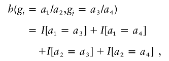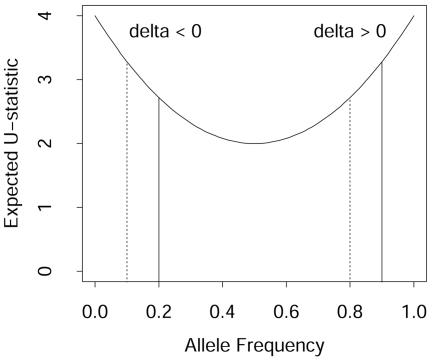
where I[…] is the indicator function having a value of 1 or 0 according to whether its argument is true or false. This kernel ranges from 0, for no matches, to 4, when a pair of subjects have the same homozygous genotype. On the surface, this similarity kernel is appealing, because one could easily extend it to multiple alleles and multiple markers (summing the allele-match scores across markers). However, further consideration shows that it can have undesirable properties when summing across markers and contrasting between cases and controls. The main issue is that the expected value of this allele-match kernel is symmetric about its minimum value, which occurs when all alleles at a marker have the same frequency. For example, consider a diallelic marker, with one of the alleles having frequency p. Under the assumption of Hardy Weinberg proportions for the genotypes, the expected value of the allele-match kernel is μ_allelematch=4-8p(1-p). This expectation is illustrated in figure 1, which shows that it is symmetric around 0.5. In this figure, we also plot solid vertical lines for cases and broken vertical lines for controls, for hypothetical allele frequencies such that cases have higher allele frequencies than controls. These vertical lines illustrate that when allele frequencies are <0.5, the difference in the mean scores between cases and controls (“delta” in fig. 1) will be negative. In contrast, when allele frequencies are >0.5, the delta will be positive. Summing over these two hypothetical markers is equivalent to summing over deltas of opposite signs and hence eliminates any potential signal for the association. It can be shown that a similar problem exists when there are more than two alleles at a marker, with the expected kernel score having its minimum value when alleles are equally frequent. That is, similarity is smallest when genotypes have the greatest amount of variability, which occurs when alleles are equally frequent. Hence, comparing average similarities between cases and controls will be influenced by how much the allele frequencies depart from equality within a group, potentially eliminating a signal when summing these allele-match kernels across markers.

Figure 1.

Expected value of U-statistic, μ, for the allele-match kernel versus allele frequency (under the assumption of Hardy-Weinberg proportions of genotypes). For hypothetical allele frequencies, the vertical solid lines represent cases and the vertical broken lines represent controls, illustrating that differences in expected kernels (delta) between cases and controls can change sign according to whether allele frequencies are less than or greater than 0.5.

Because of the problems with the allele-match kernel, we consider an alternative approach. One can score each subject’s genotype separately, by a dosage function d(g), and then sum these dosage functions for a pair of subjects to create a kernel, h(g_i,g_j)=d(g_i)+d(g_j). For example, for diallelic markers, one can count the number of alleles of a specific type, such as the more rare allele, to create the linear dosage score d(g)=0,1,2. This “linear-dosage” kernel, along with the above allele-match kernel, and a few other kernels based on the sum of other dosage functions, are illustrated in table 1. Before we describe how to determine an optimal kernel for a specified genetic effect, we show in the next section that the “sum-dosage” kernel, h(g_i,g_j)=d(g_i)+d(g_j), with an arbitrary dosage score d(g), leads to a U-statistic that is equivalent to Armitage’s trend statistic for proportions. This relationship provides an intuitive guide on the choice of kernels.

Table 1.

Examples of Kernels for Genotypes g_i and g_j

	gj
gi	a/a	a/b	b/b
	Allele Match
a/a	4	2	0
a/b	2	2	2
b/b	0	2	4
	Linear Dosage
a/a	0	1	2
a/b	1	2	3
b/b	2	3	4
	Dominant
a/a	0	1	1
a/b	1	2	2
b/b	1	2	2
	Recessive
a/a	0	0	1
a/b	0	0	1
b/b	1	1	2
	Quadratic
a/a	2	3	5
a/b	3	4	6
b/b	5	6	8

Relationship of Contrast of Within-Group U-Statistics with Armitage’s Test for Trend

Armitage’s test for trend in proportions is frequently used to compare the genotype frequencies between cases and controls. For diallelic markers, the 2 × 3 table for affection status by genotype category can be arranged as in table 2. Armitage's trend statistic measures a trend in proportions, weighted by a general measure of exposure dosage, d_i. Armitage’s trend statistic can be expressed as , where

and summations are over all possible genotypes. The statistic Z_Arm has an approximate standard normal distribution.

Table 2.

Contingency Table for Computing Armitage’s Test for Trend

	a/a	a/b	b/b	Total
Cases	r0	r1	r2	R
Controls	s0	s1	s2	S
Total	n0	n1	n2	N

A common way to score the genotypes is to let d_i=0,1,2, according to the count of the number of rare b alleles. For this type of scoring, Z²_Arm reduces to Pearson’s χ² statistic for the 2 × 2 table that compares allele counts between cases and controls when the genotypes are in Hardy-Weinberg proportions (Devlin and Roeder 1999), yet the Z_Arm statistic is robust to departures from Hardy-Weinberg proportions (Sasieni 1997). Furthermore, Z²_Arm is the score statistic from logistic regression, when the independent covariate for the genotypes is coded as 0, 1, or 2 for the number of copies of allele b. The power of Armitage’s statistic depends on how close the chosen scoring of genotypes matches the true genetic effect (Slager and Schaid 2001). For example, if allele b is dominant, then the most powerful scoring is d=0,1,1 for genotypes a/a , a/b, and b/b. For a recessive effect of allele b, the corresponding scoring should be d=0,0,1. For an additive effect on the log odds ratio, the most powerful scoring is linear, d_i=0,1,2.

When there are only two alleles at a marker, it can be shown that Armitage’s trend test is a special case of our δ contrast statistic that contrasts the within-group U-statistic for cases with that for controls when a particular kernel is used. Let d(g_i) denote the dosage scoring of genotype g_i for Armitage’s trend test. Then, if the kernel is defined to be the sum of these genotype dosage scores, h(g_i,g_j)=d(g_i)+d(g_j), it can be shown that the numerator of Armitage’s trend test, T, and δ=U_d-U_c have the relationship T=δC, where C=RS/(2N). Furthermore, Var(T)=Var(δ)C², so that the standardized statistics are equivalent. This equivalence allows us to determine the most powerful kernels for the U-statistics, by first choosing d(g) for a specified genetic effect and then converting this to a sum kernel.

Kernels that Maximize Power

Power depends on the choice of kernel, as well as the distribution of genotypes for cases and controls. Let Q₀, Q₁, and Q₂ denote the genotype probabilities for the controls having genotypes a/a, a/b, and b/b, respectively. Let P₀, P₁, and P₂ denote the corresponding genotype probabilities for the cases. These probabilities correspond to the layout of table 2. The probabilities for the cases can be expressed in terms of odds ratios and the genotype probabilities for the controls. Let ψ₁ and ψ₂ denote the odds ratios for genotypes a/b and b/b, relative to genotype a/a. Then,

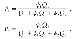and, of course, P₀=1-P₁-P₂. When the appropriate genotype probabilities are used, the expected value of δ is μ_d-μ_c, where μ is the expected value of the U-statistic, as illustrated in equation (3), evaluated with either the case or control genotype probabilities. The variance term, σ², is computed according to equation (4). Because the variance term is computed under the null hypothesis by pooling cases and controls, we use the average of the genotype probabilities for cases and controls (e.g., [P+Q]/2 for equal numbers of cases and controls) in the variance formula. Under the assumption that the number of cases, n, is equal to the number of controls, the power for a one-sided test (δ>0) is 1-Φ(z_β), where Φ is the cumulative distribution function for a standard normal distribution,

and z_α is the (1-α) quantile of the standard normal distribution. It is clear from the above expression that power is maximized by maximizing δ/σ. For a given distribution of genotypes for controls and specified genotype odds ratios, the goal is to determine which values of the kernel maximize δ/σ. We accomplish this by using the simplex method (Press et al. 1992). This method is used to find parameters that minimize a general function; in our case, we minimize -(δ/σ)². Because multiple solutions give the same minimum and, hence, the same power, we restricted the kernels to be nondecreasing as genotype similarity increases. That is, for kernels displayed as in table 1, we require that the elements within a row do not decrease as we read from left to right, and elements within a column do not decrease as we read from top to bottom. We applied this approach to a variety of genetic models, including rare and common alleles (i.e., those with disease allele frequencies equal to 0.05 or 0.25, respectively), and dominant, recessive, or multiplicative effects of the disease allele. These effects were modeled by the odds ratios, with dominant having ψ₁=ψ₂=ψ, recessive having ψ₁=1, ψ₂=ψ, and multiplicative having ψ₂=ψ²₁, with ψ₁=ψ, and ψ having a value of either 2 or 4. In all cases, we could not find kernels with greater power than those predicted by the corresponding “sum” kernels, as outlined in the previous section.

To illustrate the relative efficiency of the different sum kernels for different genetic models, we present in table 3 the relative efficiencies of a variety of kernels. The kernels “dominant,” “recessive,” and “linear” are based on the dosage functions d(g) defined in the previous section. The “quadratic” kernel is based on d(g)=1,2,4. The relative efficiencies in table 3 are presented such that the kernel with greatest power has a value of 1. The interpretation of a less-efficient kernel is that the sample size would need to be increased by 1/e, where e is the relative efficiency in table 3. The results in table 3 illustrate that when a recessive kernel is used for a dominant effect, there is a large loss in efficiency, and vice versa. The linear kernel performs best for multiplicative models (i.e., log-additive effects) and performs well for dominant effects but poorly for recessive effects. Although the quadratic kernel is not the most efficient for any of the presented models, it is fairly robust, performing reasonably well for most genetic models, except for rare recessive effects. This suggests that the quadratic kernel may be a reasonable choice when the true underlying genetic effect is unknown—a frequent situation.

Table 3.

Relative Efficiency of Different Kernels for Different Genetic Effects

	Relative Efficiency for Kernela
Model, ψ,and P	Dominant	Recessive	LinearDosage	Quadratic
Dominant:
ψ = 2:
.05	1	.15	.99	.95
.25	1	.27	.91	.79
ψ = 4:
.05	1	.14	.99	.95
.25	1	.25	.9	.76
Recessive:
ψ = 2:
.05	.19	1	.37	.52
.25	.35	1	.7	.85
ψ = 4:
.05	.24	1	.46	.62
.25	.41	1	.77	.89
Multiplicative:
ψ = 2:
.05	.99	.35	1	.98
.25	.91	.69	1	.96
ψ = 4:
.05	1	.4	1	.95
.25	.89	.76	1	.96

^aRelative efficiency is the ratio of noncentrality parameters, where a noncentrality parameter for a specified kernel is δ/σ.

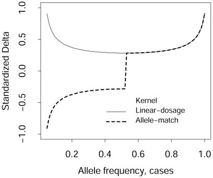
Although not immediately obvious, the allele-match kernel and the linear-dosage kernel give the same statistic for a diallelic marker, except that the sign of the statistics can differ, depending on the allele frequencies for cases and controls. This follows from the symmetry in figure 1 for the allele-match kernel, whereas the linear-dosage kernel has expected value μ_lineardosage=4p, which is a straight line with slope 4, and so avoids the complications when adding contrasts between cases and controls across markers. Without showing all the detailed algebraic derivations, it can be shown that the ratio of δ/σ for the allele-match kernel over that for the linear-dosage kernel is equal to −1 if (p_d+p_c)<1 and is equal to +1 if (p_d+p_c)>1, where p_d and p_c are the frequencies of one of the alleles for the cases and controls. In figure 2, we plot δ/σ for both kernels, for p_c=p_d-0.05. This illustrates that the absolute magnitudes of the statistics are equal, yet different in sign, when the allele frequencies for cases and controls are both <0.5. This again emphasizes caution when the allele-match kernel is being used for multiple markers.

Figure 2.

Standardized δ/σ for the allele-match and linear-dosage kernels, under the assumption that the allele frequency for controls is p_d-0.05, where p_d is the allele frequency for cases (X-axis).

Simulations

A series of simulations were used to evaluate the type I error rates and the power of our proposed Z_global statistic, relative to the power of the maximum of the single-marker tests with Bonferroni correction for multiple testing (denoted as “max-single”), and the power of Hotelling’s T² multimarker multivariate statistic (denoted as “multimarker”). The genotypes for 10 independent markers were simulated, and, of these 10, the number of markers associated with disease ranged from 0 (to evaluate the type I error rate) to 10. The frequency of the high-risk allele, for all markers, was set to either 0.05 or 0.10 (denoted in our tables as “MAF,” for “minor allele frequency”). Hardy-Weinberg proportions were used to generate the genotypes for the controls, and the genotypes for cases were generated by assuming that the high-risk allele had a multiplicative effect on the odds ratio. The effect per allele was set at either 1.25 or 1.5. The total sample size was set to either 500 or 1,000 individuals, of which half were cases and half were controls. Two-sided tests were used, and all simulations were based on 1,000 replicates.

The type I error rates for all three of the test statistics, calculated using a variety of kernels for Z_global, are presented in table 4. Almost all type I error rates for Z_global and multimarker are within the 95% CIs for the nominal error rates (α=0.01, 95% CI 0.004–0.016; α=0.05, 95% CI 0.036–0.064), suggesting that the normal distribution is adequate for the null distribution of Z_global and that the χ² distribution is adequate for multimarker. For the max-single statistic, the type I error rates are also adequate, except for the recessive kernel, which was overly conservative (most likely because of the sparseness of homozygotes for the more rare allele).

Table 4.

Type I Error Rates for max-single, multimarker, and Z_global Statistics

	Type I Error Rate for
α, Kernel, MAF,and N	max-single	multimarker	Zglobal
α = .01:
Linear dosage:
MAF = .05:
500	.005	.007	.008
N = 1,000	.009	.008	.01
MAF = .10:
N = 500	.011	.01	.009
N = 1,000	.013	.013	.01
Quadratic:
MAF = .05:
N = 500	.002	.008	.021
N = 1,000	.01	.011	.018
MAF = .10:
N = 500	.009	.009	.014
N = 1,000	.003	.009	.008
Dominant:
MAF = .05:
N = 500	.005	.007	.009
N = 1,000	.009	.01	.012
MAF = .10:
N = 500	.009	.008	.018
N = 1,000	.006	.008	.008
Recessive:
MAF = .05:
N = 500	0	.009	.005
N = 1,000	0	.011	.006
MAF = .10:
N = 500	0	.005	.003
N = 1,000	0	.012	.007
α = .05:
Linear:
MAF = .05:
N = 500	.034	.042	.041
N = 1,000	.051	.057	.055
MAF = .10:
N = 500	.056	.058	.042
N = 1,000	.053	.061	.06
Quadratic:
MAF = .05:
N = 500	.05	.055	.048
N = 1,000	.047	.046	.047
MAF = .10:
N = 500	.041	.039	.055
N = 1,000	.054	.05	.061
Dominant:
MAF = .05:
N = 500	.053	.054	.048
N = 1,000	.038	.047	.038
MAF = .10:
N = 500	.048	.038	.06
N = 1,000	.047	.043	.046
Recessive:
MAF = .05:
N = 500	0	.056	.034
N = 1,000	0	.046	.031
MAF = .10:
N = 500	0	.042	.056
N = 1,000	.017	.051	.062

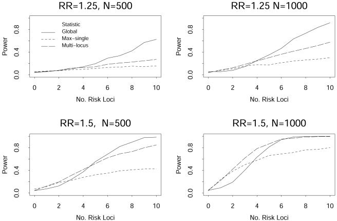
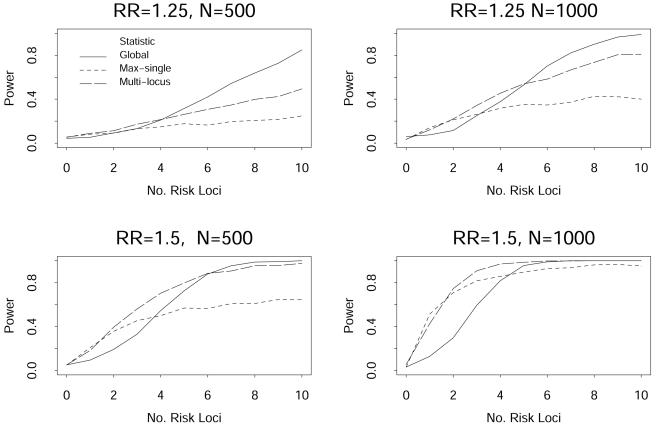
The power of the linear kernel for Z_global, the max-single statistic, and the multimarker statistic, with a type I error rate of 0.05, are presented in figure 3 for high-risk allele frequencies of 0.05 and in figure 4 for high-risk allele frequencies of 0.10. The X-axis presents the number of high-risk markers, ranging from 0 to 10. These figures illustrate that, as the number of high-risk markers increases, there is a gain in power of the Z_global statistic over the max-single and multimarker statistics, and that the gain is greatest when the effect size of the high-risk allele is not large (odds ratio per allele of 1.25 in the figures). The benefit of using the Z_global statistic seemed to occur when there were >3 high-risk markers among the set of 10 markers in these simulations. In contrast, when there were only one or two high-risk markers, the max-single and multimarker statistics had greater power than the Z_global statistic. This was most accentuated when both the allele effect size and the sample size were large (see lower right panel of fig. 4).

Figure 3.

Power from simulated data with the number of high-risk markers ranging from 0 to 10 among 10 markers, with a minor allele frequency of 0.05 for each marker.

Figure 4.

Power from simulated data with the number of high-risk markers ranging from 0 to 10 among 10 markers, with a minor allele frequency of 0.10 for each marker.

Although our simulation results show the potential gain in power provided by the Z_global statistic, our simulations are somewhat unrealistic, assuming no interactions among the high-risk markers. Simulating true biological mechanisms is also unrealistic, given our limited knowledge of underlying genes influencing complex disease. So, to evaluate how our methods behave in the presence of interactions, we consider two extreme scenarios. For the 10 markers, there are 45 possible pairwise interactions. In the first scenario, we simulate from a logistic model that has no main effects, but all 45 pairwise interactions contribute to the logistic regression model according to x_kx_lβ, where x_l and x_l are the linear dosage scores for the rare alleles at markers k and l, and β is the log odds ratio for the interaction effect; we allow the interaction odds ratio to be either 1.1. or 1.25. In the second scenario, we also assume no main effects, but 22 of the interactions have positive values of β and 23 have negative ones. That is, half the interactions increase disease risk, and the other half decrease disease risk. The results from these simulations are presented in table 5. When all interactions are positive, the Z_global statistic has a substantial power advantage over the other methods. This is likely because all methods are picking up some signal from the main effects of each marker (main effects and pairwise interactions are correlated), but the signal of each main effect is weak, so the weighted average over all markers strengthens the signal. In contrast, the model with half-positive and half-negative interactions creates main effects that have opposite signs, so that the weighted average for Z_global is near zero. Note that max-single and multimarker also have weak power for this interaction model.

Table 5.

Simulated Power for Pairwise Interaction Models

	Simulated Power for
Model, MAF,and OddsRatio	max-single	multimarker	Zglobal
All positive:
MAF = .05:
1.1	.054	.022	.104
1.25	.104	.050	.522
MAF = .10:
1.1	.135	.73	.503
1.25	.614	.595	.998
Half positive:
MAF = .05:
1.1	.044	.014	.049
1.25	.070	.027	.060
MAF = .10:
1.1	.077	.045	.052
1.25	.265	.194	.062

Application to Prostate Cancer Candidate Genes

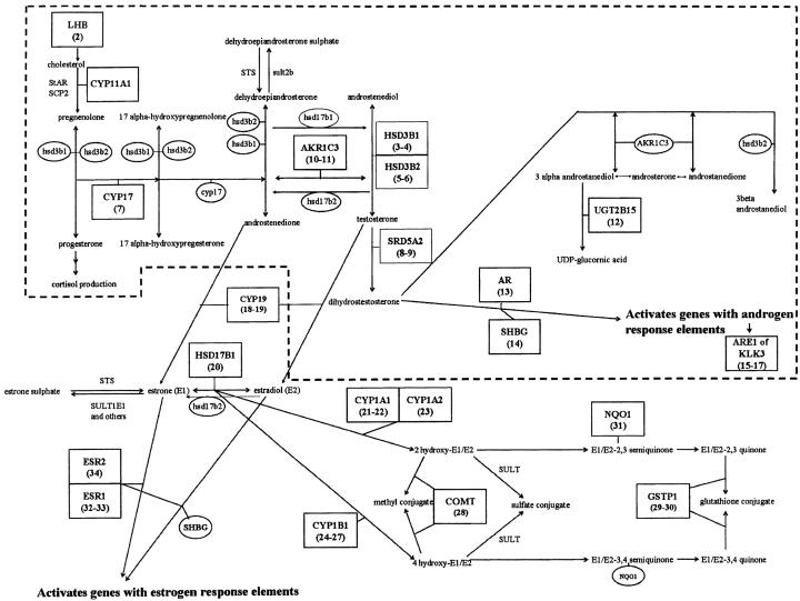
To evaluate common genetic polymorphisms for genes that are likely to be associated with prostate cancer, we measured common variations of single nucleotide polymorphisms (SNPs), chosen such that the minor allele frequency was expected to be at least 5%, in order to have adequate power to detect moderate associations. A total of 499 cases and 493 controls were recruited. We have focused on two biologic pathways: (1) 17 SNPs for genes that encode enzymes in the androgen metabolic pathway and (2) 17 SNPs for genes that encode enzymes involved in the estrogen metabolic pathway (authors' unpublished data). These two pathways are presented in figure 5. The 34 SNPs are identified by numbers within boxes, with their corresponding gene labels. Note that some genes have multiple SNPs measured; these were at different sites within the gene, at positions where prior reports suggested that variants might be associated with the risk of prostate cancer. This figure also illustrates that these two pathways have some biological links, although we analyze them separately.

Figure 5.

Candidate genes that are involved with the metabolism of androgen and estrogen. The androgen portion of the pathway is within the broken line, and the estrogen pathway is outside of the broken line, at the bottom of the figure. The measured SNPs are indicated within boxes, with their corresponding genes labeled and the SNPs numbered below each gene. Other genes and enzymes that are part of the pathway are also illustrated, emphasizing that the measured SNPs are for genes whose products act at different steps of androgen and estrogen biosynthesis.

The association of all SNPs within a pathway with prostate cancer status was evaluated with the global statistic Z_global, using different types of kernels. The results of these global tests are presented in table 6. No tests for the androgen pathway SNPs showed statistically significant associations. For the estrogen pathway SNPs, the quadratic kernel resulted in a statistically significant association (P=.028), and the linear kernel was marginally significant (P=.074).

Table 6.

Global Tests of Association of All SNPs within a Pathway with Prostate Cancer Status

	Global P for Kernel
Pathway	Linear Dosage	Quadratic	Dominant	Recessive
Androgen	.590	.706	.395	.958
Estrogen	.074	.028	.281	.654

Although our proposed methods control the overall type I error rate, interpretation of a significant global test can be difficult. To evaluate which markers “explain” the significance of the global test, we performed a stepwise procedure. Intuitively, we expect that removal of the markers that explain the statistical significance of the global test should result in nonsignificance of the remaining markers. However, because the statistical tests can be correlated, we account for this by conditioning on the removed markers when evaluating the markers that are kept. Furthermore, because the global statistic is computed under the null hypothesis, all computations of the stepwise adjusted statistics are also computed under the null hypothesis, to evaluate which markers are the most influential. To start, the marker with the smallest single-marker P value is removed, and a global test for the remaining markers is performed, adjusted for the removed marker. To determine the next marker to remove, we create a test statistic for each of the kept markers, with each statistic adjusted for the set of removed markers, and then remove the marker that has the smallest P value. After a marker is removed, a global test is performed for the kept markers, adjusted for all of the removed markers. This process is continued until the global adjusted test is no longer significant. To illustrate this adjustment procedure, partition the δ vector into the markers kept and removed, δ=(δ_k,δ_r), where the subscripts k and r denote “kept” and “removed,” respectively. Partition the null variance matrix accordingly, into submatrices V_k,k, V_k,r, and V_r,r. From multivariate normal theory, under the null hypothesis, the distribution of δ_k conditional on δ_r is multivariate normal with mean vector

and variance matrix

We use the adjusted covariance matrix V_k.r to define the weight vector w_k.r, to compute the global statistic for the kept markers, adjusted for all the removed markers,

To determine the next marker to remove, adjusted for all markers removed at prior steps, we use the statistic for the ith single marker, adjusted for the previously removed markers,

Both the single-marker–adjusted and global-adjusted statistics have an asymptotic standard normal distribution.

The results from the first three steps of removing “explanatory” SNPs are presented in table 7, for the linear and quadratic kernels. The global statistics are adjusted for the all the previously removed SNPs. For comparison, we also present the marginal single-marker P values, not adjusted for other SNPs and not adjusted for multiple testing. The Bonferroni correction would require the marginal single-marker P values to be <0.0029 to achieve statistical significance, which none of our SNPs achieved. In contrast, the global test for the quadratic kernel, at step 0, demonstrates statistical significance, emphasizing the benefit of our global test. On the basis of the quadratic kernel, it appears that the SNPs HSD17B1 and NQ01 have the most influence on the global test, since conditioning on these two SNPs, the global test has a P value of 0.111; the SNP CYP1A1 may also have some influence, although the statistical evidence is weaker. Similar evidence, although not as dramatic, is provided by the linear kernel.

Table 7.

Global Tests Adjusted for SNPs Removed Sequentially, as well as Marginal P Values for Single-Marker Tests (Not Adjusted for Multiple Testing)

		P Value
		Global		Single Marker
Step	SNP Removed	LinearDosage	Quadratic	LinearDosage	Quadratic
0	None	.074	.028
1	HSD17B1 (20)	.143	.053	.018	.034
2	NQ01 (31)	.252	.111	.048	.049
3	CYP1A1 (21)	.510	.339	.140	.123

Discussion

Common diseases are expected to be controlled by complex genetic mechanisms, with small-to-moderate effect sizes per gene, because of natural selection having removed those genes with large effects. Given the large body of evidence indicating that metabolic pathways are likely to play a major role in complex diseases and that these types of pathways have complex interactions and feedback loops, it would not be surprising to find that multiple genes within a biologic pathway are associated with disease, complicated by both allelic and locus heterogeneity. Recognizing that testing the association of disease with one marker at a time can have weak power due to small genetic effects and the need to correct for multiple testing, we have proposed a class of U-statistics that combine information from multiple genetic markers. This combined statistic achieves its greatest power when the contrasts of the within-group genetic scores between cases and controls are in the same direction across multiple markers.

The multimarker Hotelling’s T² statistic is limiting, because it does not allow for missing genotypes at some markers and does not combine information across markers into a single-df statistic, which would have less power than our proposed methods when the effects of genotypes are in the same direction across markers. Hence, an advantage of our approach is that it provides a mechanism to handle missing data while combining results from multiple markers.

Another advantage of our methods is the general framework to consider alternative types of kernels. The allele-match kernel has intuitive appeal but can be limiting, because it is influenced by how much allele frequencies differ from equality within a group—which, in turn, can cause contrasts between cases and controls to differ in sign across markers. Further work is needed to evaluate the best kernels when there are multiple alleles per marker. To provide guidance on the choice of kernel, we have illustrated how to compute the power for a given type of kernel and a specified genetic effect size (e.g., in terms of control genotype frequencies and genotype odds ratios). Our numerical comparisons suggest that the quadratic kernel is fairly robust, in the sense that it does not lose as much power as other kernels, despite not giving the greatest power.

All of our proposed kernels are additive across markers. The benefit of an additive kernel is that it can easily handle missing marker data, which is a common occurrence. Furthermore, weighted averages can be easily computed, where the weights are data driven, with the optimal weights determined by BLUEs. This strategy has been used elsewhere in genetics, such as in the use of generalized least squares to derive BLUEs of allele frequencies from pedigree data (McPeek et al. 2004). Weighted global statistics have been also used to derive optimal nonparametric statistics to compare two treatment groups over multiple endpoints (O’Brien 1984; Wei and Johnson 1985). Further work is warranted to determine if more powerful kernels can be found, such as kernels that are nonlinear over the genetic markers. For example, kernels that increase exponentially with the number of rare variants across multiple markers might be more sensitive to situations in which multiple rare variants are required for disease, suggesting higher-order interactions among markers.

A potential advantage of our approach is that linkage disequilibrium among markers is implicitly accounted for by the covariance matrix of the U vectors. This allows our methods to be used in evaluating the association of multiple markers within a candidate gene with disease. A potential limitation is that we do not evaluate the association of haplotypes (i.e., particular combinations of alleles on a chromosome) with disease, as others have proposed (Tzeng et al. 2003b). However, carefully selected SNPs that “tag” a haplotype can reduce the number of SNPs that are required to be genotyped, and analyzing these types of markers jointly—yet without regard to haplotype phase—can increase the power over haplotype analyses, because of the reduced degrees of freedom for joint marker analyses relative to the many degrees of freedom for haplotype analyses (Chapman et al. 2003). If all contrasts of marker scores between cases and controls are in the same direction, then our global statistic with 1 df will have even greater power, as is demonstrated by our simulations.

Our simulations suggest that the global statistic maintains the appropriate type I error rate and that the power of the global statistic is greater than both single-marker and multimarker tests when there are more than just a few associated genetic markers. Application to our prostate cancer study illustrates the potential gain of our global test by providing significant results that would not be found significant by use of single-marker tests with Bonferroni correction. However, this example also illustrates that, once found, a significant global test can be difficult to interpret, because it is not immediately clear which markers are driving the statistical significance. To guide our interpretation, we used a stepwise removal of the markers that had the smallest single-marker P value, with recomputation of an adjusted global test after each marker was removed. This process helped to identify a few markers that seemed to contribute the most to the global test. Further work regarding the statistical properties of the proposed stepwise procedure might be beneficial, since many stepwise selection procedures are known to have some difficulties identifying the most important subsets. Cross validation, to determine the ability to replicate the most important subset of explanatory markers, may offer guidance.

In summary, we have proposed a novel class of U-statistics that provide a simultaneous test of association of multiple genetic markers with disease. Our approach is quite general, allowing a wide variety of kernels to be used. Simulations demonstrate that our approach can be more powerful than standard methods, and application to our prostate cancer study illustrates the potential merits of our statistics, as well as their interpretations.

Software

Software that implements the methods described in this manuscript is written in the S programming language as a package called multigene, which runs in both S-PLUS and R computing environments. The package will be available from our Web site (http://mayoresearch.mayo.edu/mayo/research/biostat/schaid.cfm) and, for R users, from the Comprehensive R Archive Network site (http://cran.us.r-project.org).

References

- Chapman JM, Cooper JD, Todd JA, Clayton DG (2003) Detecting disease associations due to linkage disequilibrium using haplotype tags: a class of tests and the determinants of statistical power. Hum Hered 56:18–31 10.1159/000073729 [DOI] [PubMed] [Google Scholar]
- Conti DV, Cortessis V, Molitor J, Thomas DC (2003) Bayesian modeling of complex metabolic pathways. Hum Hered 56:83–93 10.1159/000073736 [DOI] [PubMed] [Google Scholar]
- Devlin B, Roeder K (1999) Genomic control for association studies. Biometrics 55:997–1004 10.1111/j.0006-341X.1999.00997.x [DOI] [PubMed] [Google Scholar]
- Fan R, Knapp M (2003) Genome association studies of complex diseases by case-control designs. Am J Hum Genet 72:850–868 [DOI] [PMC free article] [PubMed] [Google Scholar]
- Hoeffding W (1948) A class of statistics with asymptotically normal distribution. Ann Math Statist 22:165–179 [Google Scholar]
- Kowalski J (2001) A nonparametric approach to translating gene region heterogeneity associated with phenotype into location heterogeneity. Bioinformatics 17:775–790 10.1093/bioinformatics/17.9.775 [DOI] [PubMed] [Google Scholar]
- Kowalski J, Pagano M, DeGruttola V (2002). A nonparametric test of gene region heterogeneity associated with phenotype. Am J Stat Assoc 97:398–408 10.1198/016214502760046952 [DOI] [Google Scholar]
- Longmate JA (2001) Complexity and power in case-control association studies. Am J Hum Genet 68:1229–1237 [DOI] [PMC free article] [PubMed] [Google Scholar]
- McPeek MS, Wu X, Ober C (2004) Best linear unbiased allele-frequency estimation in complex pedigrees. Biometrics 60:359–367 10.1111/j.0006-341X.2004.00180.x [DOI] [PubMed] [Google Scholar]
- O’Brien PC (1984) Procedures for comparing samples with multiple endpoints. Biometrics 40:1079–1087 [PubMed] [Google Scholar]
- Press WH, Teukolsky SA, Vetterling WT, Flannery BP (1992) Numerical recipes in C. Cambridge University Press, Cambridge, United Kingdom [Google Scholar]
- Pritchard JK, Cox NJ (2002) The allelic architecture of human disease genes: common disease-common variant…or not? Hum Mol Genet 11:2417–2423 10.1093/hmg/11.20.2417 [DOI] [PubMed] [Google Scholar]
- Reich DE, Lander ES (2001) On the allelic spectrum of human disease. Trends Genet 17:502–510 10.1016/S0168-9525(01)02410-6 [DOI] [PubMed] [Google Scholar]
- Sasieni PD (1997) From genotypes to genes: doubling the sample size. Biometrics 53:1253–1261 [PubMed] [Google Scholar]
- Serfling RJ (1980) Approximation theorems of mathematical statistics. John Wiley and Sons, New York [Google Scholar]
- Slager SL, Huang J, Vieland VJ (2000) Effect of allelic heterogeneity on the power of the transmission disequilibrium test. Genet Epidemiol 18:143–156 [DOI] [PubMed] [Google Scholar]
- Slager S, Schaid D (2001) Case-control studies of genetic markers: Power and sample size approximations for Armitage’s test for trend. Hum Hered 52:149–153 10.1159/000053370 [DOI] [PubMed] [Google Scholar]
- Tzeng J-Y (2003) Identification of mutations affecting liability to complex disease by the analysis of haplotypes. PhD thesis, Carnegie Mellon University, Pittsburgh [Google Scholar]
- Tzeng J-Y, Byerley W, Devlin B, Roeder K, Wasserman L (2003a) Outlier detection and false discovery rates for whole-genome DNA matching. Am J Stat Assoc 98:236–246 10.1198/016214503388619256 [DOI] [Google Scholar]
- Tzeng J-Y, Devlin B, Wasserman L, Roeder K (2003b) On the identification of disease mutations by the analysis of haplotype similarity and goodness of fit. Am J Hum Genet 72:891–902 [DOI] [PMC free article] [PubMed] [Google Scholar]
- Weeks DE, Lange K (1988) The affected-pedigree-member method of linkage analysis. Am J Med Genet 42:315–326 [PMC free article] [PubMed] [Google Scholar]
- Wei LJ, Johnson WE (1985) Combining dependent tests with incomplete repeated measurements. Biometrika 72:359–364 [Google Scholar]
- Zondervan KT, Cardon LR (2004) The complex interplay among factors that influence allelic association. Nat Rev Genet 5:89–100 10.1038/nrg1270 [DOI] [PubMed] [Google Scholar]