

Abstract
The Saguenay–Lac St-Jean population of Quebec is relatively isolated and has genealogical records dating to the 17th-century French founders. In 120 extended families with at least one sib pair affected with early-onset hypertension and/or dyslipidemia, we analyzed the genetic determinants of hypertension and related cardiovascular and metabolic conditions. Variance-components linkage analysis revealed 46 loci after 100,000 permutations. The most prominent clusters of overlapping quantitative-trait loci were on chromosomes 1 and 3, a finding supported by principal-components and bivariate analyses. These genetic determinants were further tested by classifying families by use of LOD score density analysis for each measured phenotype at every 5 cM. Our study showed the founder effect over several generations and classes of living individuals. This quantitative genealogical approach supports the notion of the ancestral causality of traits uniquely present and inherited in distinct family classes. With the founder effect, traits determined within population subsets are measurably and quantitatively transmitted through generational lineage, with a precise component contributing to phenotypic variance. These methods should accelerate the uncovering of causal haplotypes in complex diseases such as hypertension and metabolic syndrome.
Introduction
Hypertension, present in 10%–35% of humans, is one of the principal risk factors for cardiovascular disease in the United States, Canada, and other industrialized nations (Franklin et al. 2001; Joffres et al. 2001). Together with obesity and dyslipidemia, it represents a significant proportion of the global and regional burden of diseases (Ezzati et al. 2002). These three entities are frequently present together and are cardinal features of the metabolic syndrome (Reaven 2004). The absence of such phenotypes is associated with longevity in the offspring of centenarians (Atzmon et al. 2004). With the impending pandemic of obesity, the increasing prevalence of these conditions will contribute to the worldwide prominence of cardiovascular mortality by 2020 (Groop and Orho-Melander 2001). The etiologies of these entities are usually multifactorial and the result of polygenic interactions with the environment (Hamet et al. 1998; Pausova et al. 1999). Although effective treatments are available for hypertension and dyslipidemia (Turnbull and Blood Pressure Lowering Treatment Trialists’ Collaboration 2003), they do not address the potential causal concomitance of presentation that may, by itself, provide novel therapeutic and preventive targets.
Since tools for the resolution of polygenic diseases are now available (Lander and Schork 1994; Doris 2002), several studies have reported genomewide scans for hypertension (Caulfield et al. 2003; Jacobs et al. 2003; James et al. 2003; Ranade et al. 2003; von Wowern et al. 2003), obesity, and dyslipidemia (Loos et al. 2003; Stein et al. 2003; Tang et al. 2003; Langefeld et al. 2004; Ueno et al. 2004), adding to a much earlier and more complete resolution of the monogenic forms of hypertension (Lifton et al. 2001). However, the results have usually been limited to a few QTLs with marginally significant LOD scores and a modest contribution to overall trait variance (Samani 2003)—even the results from a recent meta-analysis of 6,245 relatives from four multicenter networks of the Family Blood Pressure Program (Province et al. 2003). The most common limiting factors include genetic and environmental heterogeneity, which lead to decreased statistical power (Glazier et al. 2002). The present study proposes an integrative approach to the resolution of complex traits. We chose hypertension and dyslipidemia as the ascertainment criteria. Furthermore, we conducted our studies on French Canadians who represent a homogeneous population who had large families until the 1940s and who, more importantly, have computerized genealogical records dating to the original 17th-century settlers (Bouchard et al. 1989; Heyer and Tremblay 1995). With a method similar to our physiological genomics strategy that was applied to a human cohort of African Americans (Kotchen et al. 2002) and to rodent models (Stoll et al. 2001), we have used an integrated multisystem phenotyping protocol to ascertain the characteristics of cardiovascular, renal, metabolic, and anthropometric features, under stringent standard operating procedures.
We report that QTLs for several components of the metabolic syndrome are clustering within the same genomic regions. By extending sequential oligogenic linkage analysis routine (SOLAR)–corrected LOD (LODcor) scores through density analysis, we were able to define sets of families with distinct contributions to several traits. A novel layered-founder approach strongly underlined the finding of ancestral causality by the demonstration of founder separability. These observations permit us to propose a “quantitative founder effect” in complex diseases.
Methods and Procedures
Family Cohort
Families were recruited from a relatively genetically differentiated population in the Saguenay–Lac St-Jean (SLSJ) area of the Canadian province of Quebec. Families were ascertained by the presence of at least one sib pair with hypertension and dyslipidemia. Sibship sizes ranged from 2 to 11 persons (mean 3.9; median 3). The affected sib pair–inclusion criteria were essential hypertension (systolic blood pressure [SBP] >140 mmHg and/or diastolic blood pressure [DBP] >90 mmHg on two occasions or the use of antihypertensive medication), dyslipidemia (plasma cholesterol ⩾5.2 mmol/liter and/or HDL cholesterol ⩽0.9 mmol/liter or the use of lipid-lowering medication), BMI <35 kg/m2, age 18–55 years, and Catholic French Canadian origin. Exclusion criteria included secondary hypertension, DBP >110 mmHg and the use of medication, diabetes mellitus, renal or liver dysfunction, malignancy, pregnancy, and substance abuse. Once the affected sib pairs were selected, all first- and second-degree relatives aged >18 years were invited to participate in the study, independent of health status. The recruited population included 120 families (mean size 7.3 persons; median size 5 persons), comprising 897 subjects and 1,617 sib pairs (259 concordant-affected, 556 discordant, and 802 nonaffected sib pairs).
Family structure was tested for consistency by calculating the probabilities of relatedness on the basis of the genotype data (M. J. Daly, personal communication). Because of the results of paternity analysis, two subjects were removed prior to linkage analysis. The SOLAR software package (version 1.7.3) was used to calculate multipoint identity by descent (MIBD) for all subjects. Errors detected by SOLAR were resolved by a review of the genotypes of subjects and/or pedigrees, after which 14 genotypes from 10 subjects were removed because of genotype data inconsistency (mostly due to mistyping). Pedigree and subject genotype reviews continued in an iterative process until MIBDs were calculated with no error messages.
The study was approved by the ethics committees at Complexe Hospitalier de la Sagamie (Chicoutimi, Quebec), Université du Québec à Chicoutimi, and the Centre hospitalier de l’Université de Montréal.
Phenotyping
All phenotyping was performed by trained personnel who followed standard operating procedures (Kotchen et al. 2000, 2002; Pausova et al. 2000, 2002). Restricted phenotyping on day 0 included taking blood samples for DNA extraction and measuring plasma lipid, fasting glucose, uric acid, sitting blood pressure (BP), and bioimpedance (RJL System) to determine water distribution and body fat mass. Anthropometric data included 3 global measures of obesity—BMI and percentage body fat (%body fat) derived from skinfolds and from bioimpedance—and 11 regional measures: 6 trunk and extremity circumferences and 5 skinfolds. Subjects without any contraindications were invited for extensive phenotyping and had their antihypertensive drugs withdrawn for 1 wk and lipid-lowering agents withdrawn for 1 mo. From 499 hypertensive subjects studied, 388 were receiving medication, which was stopped for the purposes of full phenotyping in 135 hypertensive subjects. Full phenotyping was performed for a total of 294 normotensive and hypertensive individuals.
On day 1 of extensive phenotyping, an intravenous catheter was inserted. Fasting samples were taken for the measurement of lipid, glucose, and insulin concentrations. A postural test was conducted for 60 min in the supine position followed by 10 min standing and 20 min sitting, while cardiac functions (by impedance plethysmography [SORBA Medical System]) and BP (Dynamap, Johnson and Johnson Medical) were monitored. Both impedance and BP were then measured after mental stress of mathematical tests (McAdoo et al. 1990). Insulin sensitivity was tested with Bergman’s minimal model, and insulin sensitivity and glucose effectiveness were quantified as described elsewhere (Steil et al. 1993). At the end of day 1, 24-h BP monitoring was initiated. On day 2, BP, renal blood flow by p-aminohippuric acid clearance, and glomerular filtration rate by inulin clearance were measured at baseline and after stepwise norepinephrine infusion of 0.01–0.05 μg/kg/min (Kotchen et al. 2000). Patients received a water load of 15 ml/kg plus normal saline intravenously over a 6-h period. Plasma arginine-vasopressin, atrial natriuretic factor, cyclic nucleotide (cGMP and cAMP) concentrations, and renin activity were quantified at baseline and after fluid challenge. Cardiac echographic measurements were taken on a different day.
Among all phenotypes, those that were measured and analyzed included 3 anthropometric, 3 plasma, 37 BP, 12 time-series BP, 14 cardiac (cardiac output and index), 46 impedance plethysmography, 6 echocardiography, 19 heart rate, 32 neuroendocrine, 22 renal, and 28 plethysmography-related measures. Each phenotype was tested for normality of distribution by kurtosis and skewness and by the Kolmogorov-Smirnov test. When kurtosis was >2, values were normalized by simple function transformation (i.e., transformed by log, square root, or power) (Blangero et al. 2001) and were further analyzed to decrease the likelihood of false-positive errors (e.g., by variance-components, covariance, principal-components, and bivariate analyses). Power transformation was the first choice for any phenotype containing negative numbers (e.g., delta-calculated values). All three transformations were tested, and we used the one that achieved normality without excessive loss of data points. As in the analyses by Allison et al. (1999), we accepted, on rare occasions, slight deviations from normality if it could be assumed that they would not affect the LOD score substantially. Most importantly, however, we ran 100,000 simulations to correct for such deviations from normality and to test the robustness of our results. This method is considered to be one of the best ways to deal with normality issues. When more than two groups were compared, one- or two-way analysis of variance was applied post hoc using the Tukey honest significance difference test for specific pairs of variables. The null hypothesis was rejected whenever P was <.05. Phenotype analysis screened for general covariates, including sex, age, and BMI, with stepwise removal of each covariate to test its significance.
Genotyping
DNA samples from the first 500 recruited subjects originating from 97 families were genotyped at the Broad Institute (formerly the Whitehead Institute for Biomedical Research/MIT Center for Genome Research), by use of 377 microsatellite markers, with a modified version of the Cooperative Human Linkage Center Screening Set (version 6.0) that included Genethon markers for an average of 9.1-cM coverage of the entire human genome. Details of the genotyping system can be found elsewhere (Rioux et al. 1998). Additional markers (Genethon) at a 5-cM density were used on chromosome (chr) 1q and chr 3q in a total of 810 subjects. Post hoc analysis determined a genotyping error rate of ∼0.016%.
Components of Total Variance
We estimated the individual contribution of QTLs to the trait variance. Other modeled effects included residual effects (including environmental effects) and the effects of the covariates age and sex. For these analyses, we used extended families (i.e., those not split into sib pairs). We performed oligogenic segregation analyses based on reversible-jump Bayesian Markov Chain–Monte Carlo (MCMC) methods and implemented in the computer program Loki, version 2.4.5 (available at the Pangaea Web site), as described elsewhere (Heath 1997; Daw et al. 1999; Gagnon et al. 2003).
These MCMC methods estimate model parameters, including the number of QTLs and their contribution to the trait variance, given the assigned prior distributions for each parameter in the model and the current states of all other model parameters. We applied Poisson prior distribution with a mean of 1 for the number of QTLs. We investigated several values for the prior variance of genotype effects. The choice of the best value for the genotype effects was based on the guidelines proposed by Wijsman (2002). For these analyses, posterior parameter estimates were based on average values of 501,000 iterations of this process, with every second iteration saved for computation. The first 1,000 iterations were discarded to allow for initial burn-in of the MCMC process. Several runs were performed, and the results from one representative run for each trait are presented in this article. Since the Bayesian MCMC methods were not based on a hypothesis-testing framework, P values could not be estimated.
Permutation Analysis
To test for LOD robustness, a simulation method for permutation analysis was implemented with SOLAR (Blangero et al. 2001). LOD adjustment was computed with the LODadj command, which runs a simulation of the distribution of LOD scores that can be expected under the null hypothesis of no linkage. We ran 100,000 trials, and, in each trial, a fully informative marker, completely unlinked to the trait, was simulated and the trait linkage was tested. Under the assumption of multivariate normality, the theoretical null distribution is well known. The LODadj command regresses the observed LOD scores on the LOD scores expected for a multivariate normal trait. The inverse of the slope of the regression line is the LOD adjustment. Adjusted LOD scores are reported here.
Principal-Components and Bivariate Analyses
Principal-components analysis (PCA) is a multivariate statistical method that allows the formulation of quantitatively informative linear combinations of correlated phenotypes by maximizing phenotypic or familial variance—and thus reducing the number of tests performed—by exploring only the proper linear combinations in further variance-components analyses. It is extremely effective for correlated phenotypes regulated by a common locus, and it increases the power significantly. Hence, PCA is applied to maximize the total variance. Eigen pairs of the covariance matrix accounting for 95% of the variance formed the principal components.
Both bivariate analysis and PCA can increase the power of analysis in a case of phenotypes with small or negatively correlated environmental factors and with strong genetic correlation. Although bivariate analysis explicitly models the cross correlation matrix, it also adds more parameters into the model and makes the computations extensive. On the other hand, PCA reduces the number of tests by providing linear combinations of maximum variance for further analysis. Hence, both methods can make valuable contributions.
LOD Score Density Analysis
Density functions are the integral or discrete sum of other function values over a ranked set of function arguments. A discrete example of density δ over function f is
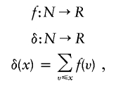 |
where x and v are the integer arguments of functions δ and f, N is the set of integer numbers, and R is the set of real numbers.
LOD score density can be computed on the basis of the LOD score contribution (LODC) of individual pedigrees, which are families in this case, as follows:
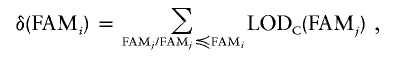 |
where
 |
and where ∨ is the logic “OR” operator, ∧ is the logic “AND” operator, and i and j are family identifiers.
In other words, LOD score density δ is computed for families ranked by decreasing values of LOD score contribution, LODC, as supplied by SOLAR from FAMi through FAMj. In the case of equal LOD contribution, the identifiers of families are arbitrarily considered for the purposes of ordering. In this context, density can also be interpreted as an incremental LOD score computation, in which families are incrementally added to the population in decreasing order of LOD score contribution.
An example of a LOD score density plot is reported in figure 1. LOD density represents the LOD score values that would be obtained if the population were restricted to families for which the density is computed. In figure 1, we can observe three regions in the density function: an initial region in which the LOD score increases as families are added to the population, a somehow stable region in which adding families does not significantly change the LOD value, and a final region in which adding families decreases the LOD score. We name the families belonging to these three regions “contributing” families (CF), “noncontributing” families (NCF), and “anticontributing” families (ACF), respectively. The families belonging to these regions can be used to assess whether they can be statistically distinguished by certain phenotypes and markers.
Figure 1.

Example of a LOD score density plot. Three regions can be observed in the density function: an initial region in which LOD score increases as families are added to the population, a somehow stable region in which adding families does not significantly change the LOD value, and a final region in which adding families decreases the LOD score.
Quantitative Founder Effect
A population is considered subject to a founder effect when a few ancestors from a set F of founders account for most of the genetic contribution to a set S of descendants. In this context, founders can be ranked on the basis of their nonuniform genetic contribution, from the highest to the lowest contributions.
An example of the genetic contribution of founders appears in figure 2A, whereas figure 2B reveals the constant genetic contribution for the contrasting hypothesis of a uniform contribution of founders. The density δ of genetic contributions is shown in figure 2C for a population subject to the founder effect, whereas figure 2D displays the density in the case of uniform distribution. In this context, density can also be interpreted as an incremental genetic contribution computation when founders are incrementally considered in decreasing order of genetic contribution.
Figure 2.

A, Genetic contribution (GC) in a population subject to a founder effect. The values represent the genetic contribution to a set of descendants prior to normalization. B, Constant genetic contribution (GC) with the hypothesis of uniform contribution of founders. Density δ of genetic contribution in a population subject to founder effect (C) and in the case of a uniform contribution of founders (D). E, Founder-effect measure interpreted as the normalized difference between the area underlying the density of genetic contribution for all founders and the area underlying the hypothetical density for a uniform contribution of founders.
Qualitatively, a more convex shape of genetic contribution density indicates that a smaller group of founders contributes to most of the genetic pool of a population. Extreme diagrams of genetic contribution density are single-founder diagrams, which result in a horizontal line corresponding to total genetic contribution gcT, and uniform-founder diagrams, which are depicted as a diagonal line from 0 to gcT. Usual cases produce convex diagrams between the two extremes.
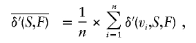
Quantitatively, the shape of genetic contribution density function δ can be expressed by its average value
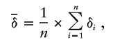 |
where n is the number of density values. When the number of founders n is large enough,  varies approximately between gcT/2 and gcT, corresponding to the cases of uniform- and single-founder contributions, respectively. In rigorous language, uniform genetic distribution density is a ladder function with steps of 1/n×gcT, whose average value is discussed in more detail in appendix A (online only).
We call founder-effect measure fe the normalized difference between  and the average uniform contribution density, as described more precisely in appendix A (online only). The founder-effect measure varies between 0 and 1, and it is equal to 0 when the founders’ genetic contributions are exactly uniformly distributed, whereas it is equal to 1 when only one founder contributes to the genetic pool.
The founder-effect measure gives an indication of the polarization and concentration of the genetic contribution from a limited number of founders. It can be used to study, in absolute terms, genetic transmission in different genealogies, or, within the same genealogy, it can compare different subpopulations with respect to the same set of founders or compare different sets of founders with respect to the same subpopulation.
Layered Founders: Ancestral Separability Method
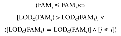
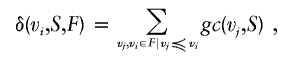
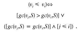
The genetic pool of the SLSJ population included in our analysis reflects its demographic history. It was shaped by its very early founders, starting in 1675 in the Charlevoix settlement and followed by migration to the SLSJ region. Until 1870, >80% of the SLSJ population came from Charlevoix, and 70% were descendants of the first three migration waves (Labuda et al. 1996). The rapid growth of the population was the result of the very large family sizes in each generation. The contribution of the later migration waves to the genetic pool diminished significantly with each generation. Such population characteristics led us to use a “genealogical graph” in which edge direction represents generational steps. We developed the layered-founder approach to overcome distortions discussed by E. Merlo, B. Deslauriers, G. Antoniol, P. L. Brunelle, M. Jomphe, G. Bouchard, O. Seda, U. Broeckel, A. W. Cowley Jr., J. Tremblay, and P. Hamet (unpublished data). Founders who share a common distance from today’s individuals constitute a layer within the geometric analogy to the concept. The first layer is the set of parents of the studied individuals, the second is that of grandparents, and so on, until the beginning of the colony. Two ancestors vi and vj belong to the same layer Lk if they are at the same distance k from today’s population, as follows:
In a given genealogy, several layers of founders can be identified, depending on the different k values of distance from today’s individuals. Since the number of generations between an ancient founder and today’s population may vary, it is possible that the maximum number of generations and the maximum number of computed layers do not coincide. Furthermore, layers also depend on the definition of distance. In work by E. Merlo, B. Deslauriers, G. Antoniol, P. L. Brunelle, M. Jomphe, G. Bouchard, O. Seda, U. Broeckel, A.W. Cowley Jr., J. Tremblay, and P. Hamet (unpublished data), several definitions of distances and layers are presented, evaluated, and discussed. The definition used in the present article is constrained average distance layered founders. Founders are specific to the class to which their genetic contribution is higher. For example, we can determine the set of founders from a layer Lk whose identical-by-descent probability p to CF is higher than their p to ACF by using a maximum-likelihood classification scheme, and we label them as “CF-specific” founders. Similarly, we can compute the mutually exclusive set of founders specific to ACF. In conceptual terms,
Technically, the previous equation has to be further detailed, as presented in work by E. Merlo, B. Deslauriers, G. Antoniol, P. L. Brunelle, M. Jomphe, G. Bouchard, O. Seda, U. Broeckel, A.W. Cowley Jr., J. Tremblay, and P. Hamet (unpublished data). Although, in absolute terms, specific founders genetically contribute to one class of descendants more than to another, the difference of contributions may be irrelevant. Indeed, there are few founders for whom the gene-transmission probability to both classes is identical. Thus, a new measure called “separability” has been introduced to capture the relevance of the difference in gene-transmission probability. In conceptual terms,
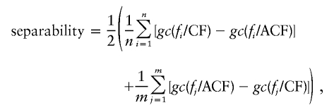 |
where n founders fi in layer Lk are specific to CF and m founders fi are specific to ACF. Separability can be thought of as the average difference in genetic contribution observed for the two sets of founders specific to either CF or ACF classes. Again, the previous equation has to be further detailed, as presented in work by E. Merlo, B. Deslauriers, G. Antoniol, P. L. Brunelle, M. Jomphe, G. Bouchard, O. Seda, U. Broeckel, A.W. Cowley Jr., J. Tremblay, and P. Hamet (unpublished data). The separability and specificity of layered founders with respect to distinct classes of families in the current generation are illustrated schematically in figure 3.
Figure 3.

Schematic illustration of separability and specificity of layered founders with respect to distinct classes of families in the current generation.
Results
General Characteristics of Subjects
BP, anthropometric, and selected metabolic data validated in 810 subjects at the time of analysis are reported in table 1, which also identifies traits that are highly significantly different between hypertensive and normotensive subjects of both sexes. These involve BP, as expected, and several anthropometric parameters, including %body fat, particularly as derived from impedance measurements. Noticeably, %body fat determined by impedance correlated significantly with %body fat calculated by skinfolds (r=0.70; P<.001), whereas the difference between normotensive and hypertensive subjects was better captured by impedance.
Table 1.
Biological Characteristics and Familial Correlations of Phenotypes, by Patient Sex and BP Status[Note]
|
Males |
Females |
|||||||||||
| With HBP(n=205b) |
Without HBP(n=166c) |
With HBP(n=262d) |
Without HBP(n=177e) |
|||||||||
| Characteristica | Mean | SE | r | Mean | SE | r | Mean | SE | r | Mean | SE | r |
| Age (years) | 51.53 | .83 | 45.30 | 1.07 | 57.37 | .74 | 42.92 | 1.05 | ||||
| SBP (mmHg) | 142.0 | 1.6 | .03 | 121.9 | 1.0 | .29 |
144.2 | 1.4 | .04 | 113.7 | 1.0 | .13 |
| DBP (mmHg) | 90.6 | .8 | .01 | 78.6 | .7 | .33 |
84.8 | .7 | .14 | 73.5 | .7 | .24 |
| Heart rate (beats/min) | 70.7 | 1.1 | .07 | 67.6 | 1.0 | .55 |
73.6 | .9 | .00 | 72.7 | .8 | .53 |
| Height (cm) | 171.0 | .5 | .56 |
173.5 | .5 | .68 |
157.6 | .4 | .46 |
160.3 | .5 | .47 |
| Weight (kg) | 82.4 | 1.0 | .28 |
79.2 | 1.2 | .31 |
68.4 | .9 | .16 | 63.5 | 1.0 | .27 |
| BMI (kg/m2) | 28.1 | .3 | .11 | 26.3 | .4 | .18 | 27.5 | .4 | .23 | 24.8 | .4 | .19 |
| Waist-to-hip ratio | .984 | .005 | .26 |
.946 | .005 | .06 | .849 | .005 | .23 | .809 | .007 | .19 |
| Waist circumference (cm) | 99.4 | .8 | .25 |
92.92 | .88 | .20 | 87.67 | .93 | .17 | 80.10 | 1.01 | .10 |
| Hip circumference (cm) | 100.7 | .5 | .23 | 98.00 | .50 | .26 |
103.1 | .7 | .10 | 99.3 | .7 | .14 |
| Thigh circumference (cm): | ||||||||||||
| Proximal | 58.2 | .4 | .28 |
57.20 | .50 | .27 |
58.8 | .4 | .10 | 59.0 | .5 | .28 |
| Mid | 43.4 | .4 | .27 |
52.60 | .50 | .23 | 52.8 | .4 | .04 | 52.4 | .5 | .30 |
| Distal | 40.9 | .3 | .20 | 39.90 | .30 | .25 |
40.6 | .3 | .07 | 39.9 | .3 | .38 |
| Skinfold (mm): | ||||||||||||
| Biceps | 16.82 | .96 | .37 |
16.61 | .98 | .12 | 23.81 | .84 | .12 | 22.13 | 1.08 | .07 |
| Triceps | 23.57 | .94 | .17 | 23.14 | 1.06 | .07 | 34.25 | .81 | .29 |
30.22 | .96 | .10 |
| Subscapular | 25.81 | .78 | .15 | 22.81 | .84 | .15 | 28.22 | .86 | .40 |
24.24 | 1.03 | .11 |
| Suprailiac | 24.90 | .94 | .41 |
21.81 | 1.02 | .03 | 27.11 | .74 | .29 |
23.72 | 1.09 | .08 |
| Thigh | 24.45 | 1.08 | .35 |
26.84 | 1.27 | .12 | 43.27 | .89 | .08 | 39.25 | 1.06 | .05 |
| Body fat (%): | ||||||||||||
| Calculated | 25.98 | .39 | .09 | 24.96 | .49 | .15 | 39.03 | .42 | .31 |
36.30 | .61 | .12 |
| Derived | 24.58 | .56 | .44 |
21.16 | .69 | .38 |
37.39 | .77 | .22 | 30.35 | .82 | .00 |
| Cholesterol (mmol/liter): | ||||||||||||
| Total | 5.53 | .09 | .06 | 5.57 | .09 | .18 | 5.75 | .08 | .19 | 5.24 | .08 | .23 |
| HDL | 1.16 | .03 | .32 |
1.20 | .02 | .43 |
1.50 | .03 | .19 | 1.54 | .03 | .00 |
| LDL | 3.34 | .07 | .42 |
3.60 | .09 | .37 |
3.31 | .07 | .16 | 3.12 | .07 | .00 |
| Triglycerides (mmol/liter) | 2.40 | .15 | .12 | 1.86 | .10 | .21 | 1.98 | .07 | .25 |
1.29 | .06 | .29 |
| Glucose (mmol/liter) | 5.79 | .12 | .00 | 5.29 | .07 | .45 |
5.40 | .07 | .19 | 4.97 | .08 | .04 |
| Creatinine (μmol/liter) | 91.7 | 2.0 | .13 | 85.9 | .9 | .03 | 70.8 | 1.1 | .03 | 68.2 | .9 | .18 |
| Uric acid (μmol/liter): | ||||||||||||
| Plasma | 356.5 | 5.6 | .17 | 331.8 | 4.6 | .25 |
295.2 | 4.6 | .21 | 245.9 | 3.8 | .29 |
| Urinary | 3.04 | .22 | .05 | 2.38 | .30 | .24 | 2.72 | .27 | .72 |
1.85 | .19 | .51 |
| Glycerol (mmol/liter) | .105 | .028 | .96 |
.053 | .004 | .04 | .099 | .004 | .44 |
.080 | .003 | .18 |
| Reactance (Ω): | ||||||||||||
| Ecw | 567.0 | 5.2 | .07 | 582.2 | 5.5 | .27 |
677.4 | 6.5 | .39 |
701.3 | 7.2 | .41 |
| Icw | 1,027.2 | 14.4 | .03 | 1,037.1 | 15.5 | .38 |
1,407.4 | 20.5 | .23 | 1,429.2 | 22.9 | .46 |
| Insulin (pmol/liter) | 134.7 | 7.1 | .11 | 114.5 | 4.6 | .32 |
112.9 | 3.3 | .04 | 103.4 | 2.6 | .31 |
| Arg-vaso (pg/ml)f | 4.45 | .17 | .33 |
4.56 | .19 | .53 |
4.55 | .16 | .22 | 4.94 | .17 | .02 |
| Renin, supine (ng/ml/h)f | 1.23 | .11 | .61 |
1.77 | .17 | .31 |
1.25 | .13 | .17 | 1.35 | .10 | .41 |
Note.— Values in bold italics indicate P⩽.001 between groups with and groups without high blood pressure (HBP); underlined values indicate correlation ⩾0.25 (i.e., h2>50%). Familial correlation r was calculated with FCOR software.
Arg-vaso = arginine-vasopressin; Ecw = extracellular water; Icw = intracellular water.
Maximum no. of sib pairs generated = 145.
Maximum no. of sib pairs generated = 77.
Maximum no. of sib pairs generated = 234.
Maximum no. of sib pairs generated = 85.
Measured in extensive phenotyping only.
Table 1 also reports familial correlations and estimates of apparent heritability (h2) calculated by the FCOR program of the SAGE statistical package. Significant correlations within sib pairs (h2=2xr and r>0.25; therefore, h2>50%) were found for SBP, DBP, and heart rate only in normotensive individuals of both sexes. It must be noted, however, that apparent heritability estimates for BP were much higher for hypertensive subjects (n=174) after the withdrawal of antihypertensive medications, increasing in males from r=0.03 to r=0.29 for SBP and from r=0.01 to r=0.22 for DBP and in females from r=0.04 to r=0.35 for SBP and from r=0.14 to r=0.37 for DBP, regardless of whether the analysis included those who were never treated for hypertension (n=293). As reported elsewhere, anthropometric measures, particularly those related to higher %body fat, exhibited higher heritability percentages in hypertensive than in normotensive subjects (Pausova et al. 2001). This was also evident for heritability estimates of serum glycerol levels (table 1).
Partitioning of Variance
To evaluate the feasibility of detecting and mapping QTLs underlying the hemodynamic, anthropometric, and metabolic traits presented in table 1, we targeted the traits with high heritability by estimating the number of large QTLs and their relative contributions to the variance for traits (table 2).
Table 2.
Partitioning of Variance of a Set of Hemodynamic, Anthropometric, and Metabolic Traits
|
Percentage of Total Variance (Square Root of Variance) Attributed to Modeled Effects |
||||||||
| QTLsa |
||||||||
| Source of Variance | Residual | Age | Sex | Total Genetic Variance | First | Second | Other | Absolute Total Variance |
| SBP (mmHg) | 44.2 (176.78) | 18.3 (73.03) | .7 (2.97) | 36.8 (147.10) | 20.8 (83.07) | 11.9 (47.44) | 4.1 (16.59) | 399.88 |
| DBP (mmHg) | 66.7 (85.30) | .8 (1.07) | 5.1 (6.45) | 27.4 (35.08) | 18.0 (23.05) | 6.7 (8.59) | 2.7 (3.44) | 127.90 |
| Weight (kg)b | 22.1 (53.38) | 3.8 (9.26) | 3.8 (9.20) | 42.2 (101.89) | 25.4 (61.20) | 10.1 (24.45) | 6.7 (16.24) | 241.30 |
| BMI (kg/m2) | 37.6 (9.61) | 1.0 (.25) | 2.2 (.55) | 59.2 (15.10) | 31.5 (8.04) | 16.3 (4.15) | 11.4 (2.91) | 25.50 |
| Waist circumference (cm) | 42.1 (91.63) | 3.2 (7.02) | 19.0 (41.24) | 35.7 (77.52) | 23.4 (50.63) | 9.7 (21.09) | 2.6 (5.80) | 217.41 |
| Skinfold subscapular (mm) | 12.1 (16.24) | .5 (.69) | .3 (.37) | 87.1 (116.85) | 41.2 (55.32) | 25.1 (33.69) | 20.8 (27.84) | 134.15 |
| HDL cholesterolc (mmol/liter) | 55.8 (.019) | .8 (.000) | 11.8 (.004) | 31.6 (.011) | 21.8 (.008) | 8.1 (.003) | 1.7 (.00) | .0343 |
| LDL cholesterol (mmol/liter) | 48.9 (.513) | 2.1 (.022) | 1.1 (.012) | 47.9 (.501) | 20.1 (.211) | 14.0 (.147) | 13.8 (.143) | 1.05 |
| 24-h urinary uric acidd (μmol/liter) | 60.9 (.086) | 1.7 (.002) | 1.9 (.003) | 35.5 (.050) | 31.9 (.045) | 3.0 (.004) | .6 (.001) | .142 |
| Body fat by impedance (%) | 22.2 (26.85) | 18.9 (22.90) | 23.6 (28.53) | 35.3 (42.72) | 20.6 (24.90) | 10.2 (12.29) | 4.5 (5.53) | 121.00 |
Ranked in order of variance contribution.
Height was added as a covariate in the analysis. The contribution of height to the variance of weight was 28.1% (67.57 kg).
Values are log10 HDL.
Values are the square root of 24-h urinary uric acid.
Estimates of variance contribution for the effects modeled (table 2) showed evidence of at least one major QTL with individual contribution in the range of 18% to >41% for several traits. There was also evidence of a second QTL with a large effect, up to ∼25% contribution, for some of these traits. Subscapular skinfolds presented evidence of the highest genetic contribution, with at least three QTLs, each with an individual contribution >20%. Our results also suggest a large contribution (∼18%) of age to the variance of SBP but not DBP, which is compatible with the well-known continuous increase in SBP with aging, in contrast to DBP, which reaches a plateau and then declines after age 55 years, as seen in this population and in a population study of 27,000 Canadians (Joffres et al. 2001), with findings similar to data from the Framingham Heart Study (Franklin 2004) and National Health and Nutrition Examination Survey III (Burt et al. 1995). Age was found to contribute, to a large extent, to the variance of %body fat measured by impedance. On the other hand, the covariate sex explained 12%–24% of the variance of waist circumference, LDL levels, and %body fat. These results thus confirmed that age and sex are important covariates for cardiovascular-related phenotypes and that a sizable sexual dimorphism has to be considered for several of these traits. The results presented in table 2 also confirmed the oligogenic and multifactorial nature of these traits, as demonstrated by the relatively large contribution of both genetic (from a few QTLs) and environmental (residual) factors to the variance. For example, the percentage of residual contribution to the variance of LDL levels was about the same as the genetic contribution—that is, ∼48%.
BMI is the most often studied phenotype in the search for genes underlying obesity-related traits. However, this trait is a compound phenotype and, therefore, is unlikely to provide accurate estimates. In addition to BMI, we also analyzed weight and modeled height in the segregation analysis. As expected, this strategy provided lower estimates for residual variance. Most of the variance of weight (78%) could thus be explained by the effects modeled for QTLs, age, sex, and height. The contribution of height to the variance of weight was ∼30%. The genetic contribution for BMI was ∼60% compared with ∼40% for weight adjusted for height, suggesting that part of the genetic variance of BMI is due to the genetic contribution of height. As defined in this data set, the phenotypes of glucose and insulin plasma levels did not show evidence for a genetic contribution (data not reported).
Genomewide Linkage
The oligogenic character of most traits under study was also evident from genomewide linkage analysis. Whereas a total of 46 LOD scores >1.9 were detected for the 213 BP, anthropometric, and metabolic traits analyzed, several of them were found in QTL clusters, particularly on chr 1, chr 3, chr 16, and chr 19 (fig. 4 and table 3). These clusters were analyzed further (see fig. 5 for chr 1, fig. 6 for chr 3, fig. 7 for chr 16, and fig. 8 for chr 19). A QTL cluster was defined as a chromosomal region in which at least one trait had a LOD score >2.0 and two additional traits with LOD scores >1.5 followed a similar pattern of linkage. When these conditions were reached, we further analyzed additional dependent and independent traits within the same chromosomal region. On chr 1, the highest LOD scores were reached for thigh circumferences (LOD of 3.8 between markers D1S1677 and D1S2878) and BMI (LOD of 3.4 at D1S2762 at 175–180 cM). Among the metabolic components, fasting insulin levels peaked at the same location, with a LOD of 2.7 at marker D1S1679. Other metabolic features, such as apolipoprotein A (apoA), apoB, leptin, and cAMP levels, were also observed in this region. Several skinfold phenotypes were localized at a somewhat more telomeric location (210–215 cM): subscapular (LOD of 3.6 between D1S1660 and D1S2622) and biceps (LOD of 3.4 at D1S2816), as were global obesity measures: %body fat by skinfolds (LOD of 3.1 at D1S2757), closely followed by %body fat by impedance (LOD of 2.9 between D1S238 and D1S3468). At an even further telomeric location (∼230 cM), several DBP traits clustered, including a peak of average DBP with a LOD of 2.1 at D1S2141 (fig. 6).
Figure 4.

Total-genome view of quantitative-trait linkage analysis by use of SOLAR in French Canadian families with hypertension and/or dyslipidemia. Phenotypes with a LOD score >1.9 after 100,000 permutations are shown. For more details, see table 3.
Table 3.
Chromosomal Positions, Phenotypes, and Maximum LOD Scores
| Chr and Position (cM) | Phenotype | LOD |
| 1: | ||
| 170 | Fasting insulin level | 2.6459 |
| 174 | Upper-arm circumference | 2.3289 |
| 176 | Thigh proximal circumference | 3.7145 |
| 176 | Thigh distal circumference | 2.6367 |
| 176 | Thigh midway circumference | 2.3725 |
| 177 | BMI | 3.3811 |
| 203 | %body fat by impedance | 2.9147 |
| 209 | %body fat by skinfold | 3.1234 |
| 210 | Triceps skinfold | 2.6783 |
| 211 | Biceps skinfold | 2.5601 |
| 213 | Suprailiac skinfold | 3.557 |
| 214 | Subscapular skinfold | 3.9321 |
| 233 | Average DBP | 2.1098 |
| 2: | ||
| 1 | BMI | 2.9129 |
| 1 | Suprailiac skinfold | 2.2282 |
| 3: | ||
| 96 | Left ventricular mass | 2.3686 |
| 101 | Extracellular body water volume | 2.123 |
| 169 | Asleep DBP | 1.9738 |
| 176 | Pre–math stress DBP | 1.9383 |
| 176 | Average DBP | 2.570 |
| 5: | ||
| 167 | Urine potassium | 2.4214 |
| 6: | ||
| 18 | Transthoracic impedance | 2.3304 |
| 109 | Urine microalbumine | 2.157 |
| 7: | ||
| 43 | Resistance | 2.4531 |
| 8: | ||
| 14 | Plasma sodium | 3.1506 |
| 48 | Cardiac output | 1.972 |
| 49 | Cardiac index | 1.9556 |
| 103 | Norepinephrine supine 55 min | 2.2157 |
| 133 | Suprailiac skinfold | 2.2973 |
| 9: | ||
| 114 | Resistance | 1.9547 |
| 11: | ||
| 83 | Intracellular water volume | 1.928 |
| 12: | ||
| 96 | Resistance | 2.1101 |
| 14: | ||
| 111 | Norepinephrine supine 55 min | 2.7012 |
| 15: | ||
| 50 | Inulin clearance after .025 norepinephrine | 2.0304 |
| 87 | Transthoracic impedance | 2.3652 |
| 16: | ||
| 50 | Awake DBP | 2.1395 |
| 50 | Awake mean BP | 2.2503 |
| 57 | Epinephrine standing 10 min | 1.9433 |
| 17: | ||
| 11 | Vasopressine | 1.9557 |
| 18: | ||
| 69 | Milwaukee index | 2.3229 |
| 79 | Extracellular body water volume | 2.2486 |
| 19: | ||
| 11 | Suprailiac skinfold | 2.2997 |
| 20: | ||
| 23 | Suprailiac skinfold | 2.1235 |
| 21: | ||
| 30 | Norepinephrine supine 55 min | 2.186 |
| 35 | BMI | 3.3539 |
| 39 | Upper-arm circumference | 3.1942 |
Figure 5.

Clusters of phenotypes illustrated by LOD curves for significant and suggestive QTLs on chr 1. A and B, Obesity-related anthropometric phenotypes. A, BMI (black line) and circumferences of thigh proximal (blackened diamonds), thigh midway (gray diamonds), thigh distal (unblackened diamonds), and upper arm (orange line with black dashes). B, Skinfolds: suprailiac (red line), subscapular (orange line), biceps (yellow line), and triceps (pink line); and %body fat by impedance (blackened circles) and by skinfolds (unblackened circles). C, Metabolic phenotypes: insulin (dark purple line), renin (blue line), leptin (blue circles), apoB (yellow line with black dashes), arginine-vasopressin (turquoise line), apoA (green line), and cAMP 24-h excretion (light purple line). D, BP-related phenotypes: average DBP (green line), awake DBP (green line with asterisks [*]), post–math stress DBP (blackened triangles), and mean awake BP (black line with asterisks [*]).
Figure 6.

Clusters of phenotypes illustrated by LOD curves for significant and suggestive QTLs on chr 3. Left panel, Sodium (yellow line), renin (blue line), mean awake BP (black line), and asleep SBP (red line with dashes). Right panel, DBP phenotypes: average (green line), awake (green line with asterisks [*]), sleep (green line with dashes), supine (green line with squares), and pre–math stress (green line with blackened triangles).
Figure 7.

Clusters of phenotypes illustrated by LOD curves for significant and suggestive QTLs on chr 16. The graph shows epinephrine (red line), average supine DBP (unblackened triangles), awake DBP (unblackened circles), mean BP (blackened triangles), SBP (line with dashes), and triglycerides (black line). “ln” indicates that the logarithmic method was used.
Figure 8.

Clusters of phenotypes illustrated by LOD curves for significant and suggestive QTLs on chr 19. “LN” indicates that the logarithmic method was used. CF = circumference.
A second major cluster was detected on chr 3 at 170–180 cM. A LOD of 2.6 was obtained for average DBP (between D3S1763 and D3S3053). The narrow peak reflected higher power, because phenotyping was conducted in all subjects, whereas other traits required the extensive phenotyping protocol described in the “Methods and Procedures” section (Kotchen et al. 2000). Thus, asleep DBP (determined by 24-h ambulatory BP monitoring [ABPM]) reached a LOD of 2.0 between D3S1746 and D3S1763, pre–math stress DBP LOD was 1.9 at D3S3053, 24-h awake DBP LOD was 1.5 at D3S1763, and average supine DBP LOD was 1.4 at D3S3053, whereas plasma renin while standing LOD was 1.4 (between D3S3053 and D3S2427). Clearly, the strength of these observations resided in the fact that they all appeared in a common, relatively narrow chromosomal segment in spite of having been measured under largely different physiological conditions.
PCA and Bivariate Data Analyses
In analyzing the findings of this study, we were faced with multivariate data recorded from extensive phenotyping. One of the approaches to deciphering the genetic architecture of these multivariable phenotypes (Ghosh and Majumder 2001) is PCA and bivariate analyses of the results, as illustrated in figure 9. For the multiple phenotypes present in the QTL clusters on chr 1 (fig. 5) and chr 3 (fig. 6), PCA was done with the correlation matrix of the phenotypes that were available on >500 subjects. For the PCA for chr 1, we included phenotypes mapping to the region with significant or suggestive LOD scores (BMI; %body fat, determined by bioimpedance; biceps, subscapular, suprailiac, and triceps skinfolds; and circumferences of proximal, middle, and distal thigh). The correlation between principal component factors and initial phenotypes was computed first, and then linkage analysis was performed for both factors, with principal component factor 1 mapping to our initial linkage region on chr 1 with a LOD score of 4.9 at position 212 cM (fig. 9A shows a LOD plot for all included phenotypes and factor 1). Bivariate analysis, including that of BMI and glucose insulin, exceeded a LOD of 5 at 175 cM on chr 1. For chr 3, in 130 subjects not receiving medication, bivariate analysis of DBP measured before the mathematical test and average asleep DBP derived from 24-h ABPM, we found a LOD significantly higher than that for both univariate analyses (LOD of 4.4), peaking at 173 cM. The same was true for the results of bivariate analysis on chr 1, in which combined BMI and insulin traits yielded a LOD of 5.1 at 173 cM.
Figure 9.

PCA and bivariate analyses of traits linked to chr 1 and chr 3. A, Linkage of principal component 1 (PC 1) (green line) on chr 1, including BMI; %body fat (determined by bioimpedance); skinfolds: biceps, subscapular, suprailiac, and triceps; and circumferences of proximal, middle, and distal thigh (for details on individual linkage results, see fig. 5). B and C, Bivariate analyses for chr 1 and chr 3. B, Univariate analyses of BMI (black line) and fasting insulin (green line) and bivariate analysis (red line). C, Univariate analyses of pre–math stress DBP (light blue line) and mean asleep DBP measured by 24-h ABPM (dark blue line) and bivariate analysis (purple line).
Classification of Families on the Basis of Their LOD Score Contributions
In complex traits, it is well known that clinical as well as genetic heterogeneity greatly hampers the uncovering of causal genomic factors. In our study population, in spite of its relative homogeneity, genetic heterogeneity was still clearly present. Although a heterogeneity-corrected LODcor obtained by SOLAR has the capacity to assess oligogenic traits, we sought additional tools to reduce the impact of locus heterogeneity. We initially deployed the LODcor obtained by SOLAR and then ranked the families by density, as described in the “Methods and Procedures” section. This approach allowed the ranking of families into CF, NCF, and ACF classes (illustrated in fig. 1), providing the possibility of uncovering loci contributing to a trait variance that would have been missed by SOLAR analysis. Indeed, our method is novel and was not previously published. To evaluate the significance of the increase in LOD scores from the baseline of 0.49 at this locus, we estimated the probability of obtaining a LOD score of 5.82 by a random selection of families. An empirical P value was computed by performing two kinds of permutation tests. In one test, the random variable is the set of CF, so we compare 10,000 random sets of 25 families to see how many times the subset generates a multipoint LOD score at least as high as the maximum subset LOD score found for CF. The P value is calculated on the basis of the proportion of 10,000 random sets of families that gave such a maximum subset LOD score. The highest LOD score generated by this method was 3.97 (mean 0.23; SD 0.35) with a corresponding P value <.0001. In the other test, we randomly ordered all the families and, beginning with the first-ranked family, we repeatedly considered larger subsets (e.g., 1, 1_2, 1_2_3, …) and computed the multipoint LOD score by adding the remaining families in order, one by one, until all families were included. The highest LOD score obtained was retained. The above operation was repeated 10,000 times, and the highest LOD score generated was 4.42 (mean 0.88; SD 0.44); thus, the P value was <.0001.
Twenty-thousand LOD score density analysis runs were performed for the entire chr 1 specific to the cluster illustrated in fig. 5, to ascertain the maximized LOD score for BP. Although many metabolic traits were observed in this cluster, only a modest contribution of BP at the more telomeric position was found (fig. 5D). Multipoint maximization selection indeed uncovered a robust LOD score for SBP on chr 1 within the metabolic cluster component. As seen in figure 10, whereas SOLAR analysis of recumbent SBP gave a LOD of 0.5 at the locus 195 cM on chr 1, 23 CF reached a LOD of 5.7, and 21 ACF had a LOD of 0. This difference in LOD scores translated into a 10-mmHg recumbent SBP phenotypic gradient between CF and ACF (P=.007, with age and sex as covariates).
Figure 10.

Approximate gradient-driven LOD score density maximization. A, LOD scores at 195 cM on chr 1 for the SBP trait in families classified by LOD score contribution. B, LOD scores at 180 cM on chr 3 for the average supine DBP trait in family classes. C, Family averages of SBP in family classes at 195 cM on chr 1. D, Family averages of supine DBP in family classes at 180 cM on chr 3. C = contributing families; N = noncontributing families; A = anticontributing families. Letter combinations reflect the joining of families in the different groups (e.g., CNA = contributing, noncontributing, and anticontributing families combined).
Similar multipoint maximization selection was performed for DBP on chr 3. Whereas the DBP QTL at 180 cM on chr 3, in the entire population, peaked at a LOD of 1.2, analysis of 15 CF increased the LOD to 2.9, and 15 ACF had a LOD of 0, accounting for the 5.5-mmHg DBP gradient between CF and ACF (P=.0003). Further analysis indicated that 22% of individuals from seven CF overlapped between the two loci, giving a Jacquard coefficient of 22% and, in fact, that only five ACF overlapped between loci on chr 2, yielding a Jacquard coefficient of 16%. The Jacquard coefficient is defined as Jc=|CF∩ACF|/|CF∪ACF|—that is, Jc is the ratio of the cardinality of the union to that of the intersection between CF and ACF. Phenotypic analysis of these CF and ACF classes demonstrated that CF sharing maximized LOD scores on chr 1 and chr 3 and that CF families, though bearing similar BP values to those of ACF families, exhibited more obesity features, including BMIs of 28 versus 24 (P=.0005), waist circumferences of 93 versus 78 (P=.002), supscapular skinfolds of 29 versus 21 (P=.003), and %body fat of 26 versus 18 (P=.01) for CF versus ACF classes. A feature of metabolic syndrome was thus apparent in 37% of CF and 9.6% of ACF classes.
Ancestral Separability of Families: The Layered-Founders Approach
At this point in our study, we sought further evidence for shared genetic determinants in the familial classes described above. The eventual ancestral relatedness of these families should constitute such an ascertainment. One of the advantages of studying the French Canadian population of the SLSJ region resides in the richness and completeness of the genealogical data collected since the beginning of the colony in 1608 and computerized in the BALSAC population register (Bouchard et al. 1989). We have used these genealogical data up to the depth of 17 generations over 14 layers of founders (see the “Methods and Procedures” section) to analyze the genetic effect of ancestors in CF and ACF classes of living subjects. The founder-effect measures vary from 0.6 to 0.7 at the most recent layer and from 0.8 to 0.9 at the oldest layer. These figures indicate that the polarization of genetic contribution is more pronounced at distant generations and is more diluted (although still relevant) at recent generations. Figure 11 illustrates that the ancestors of family classes contributing to BP QTLs on either chr 1 or chr 3 displayed a specificity >90% within the 3–4 most recent layers, and, even for the oldest layers, the expected drop maintained specificity between ∼55% and 85%. By observing founder-effect and specificity measures, one can note that these measures are conceptually and experimentally distinct. In recent layers, we discovered higher specificity and lower polarization, which indicates that genes are transmitted through paths that intersect less than in older layers (higher specificity), whereas the amount of contributions is more similar among recent founders than among older founders (lower polarization). A unique contribution to each family class exceeded 90% for the three most recent layers, and it was still 20%–30% of the most distant ancestors (fig. 11A and 11C). Figure 11B and 11D depicts the separability of classes of founders, which is the average differential contribution of separable founders to family classes and which is >80% for the 3–4 most recent layers, remaining at ∼40% for the most distant founders. Separability indicates that, for recent generations, the genetic contributions of specific founders to CF and to ACF differ by >80%, on average. For older generations, such genetic contributions differ by >40%, on average, which is still a wide gap in genetic contribution. We then proceeded “back to the future” to regroup the living descendants from the unique ancestors of CF and ACF classes of chr 1 multipoint maximized LOD at 195 cM. Within our cohort of 120 families, after eliminating families with shared ancestral contributions to individuals of both CF or ACF, we identified 25 families with 224 members with unique ancestors of the CF class (streaming out from 66 genotyped subjects) and 26 families with 213 members (62 genotyped individuals) for the ACF class. The SBP was 10 mmHg higher in CF descendants than in ACF descendants (P=.0009). These results permit the ascertainment of relevance of family classes sharing both ancestor classes and relevant phenotypes initially determined by their maximized linkage at a specific locus.
Figure 11.

A and B, Founders’ specific (squares) and unique (circles) genetic contributions to family classes, which are either contributing (blackened squares and circles) or anticontributing (unblackened squares and circles) to the LOD score. C and D, Overall separability of CF versus ACF over 14 generational layers at the corresponding loci. E and F, Founder effect (squares) and specific normalized founder effect (circles) in CF (blackened squares and circles) and ACF (unblackened squares and circles). A–C, SBP trait at 195 cM on chr 1. C–E, Average supine DBP trait at 180 cM on chr 3.
Discussion
The oligogenic and epistatic character of complex diseases makes the search for their genetic determinants a challenging task (Lander and Schork 1994; Hamet et al. 1998; Doris 2002; Glazier et al. 2002; Samani 2003). One of the approaches that has had some success is to study relatively isolated human populations, such as the Hutterites from South Dakota (Newman et al. 2003); the Finnish subpopulation from Koilliskaira, relatively isolated since the sixteenth century (Woolley et al. 2002); the Icelandic population analyzed by deCODE (Helgadottir et al. 2004); and the French Canadian population investigated in the present study (Bouchard et al. 1989), or to study populations of Mormons from Salt Lake City because of their unifying religious, nutritional, and genetic characteristics (Jeunemaître et al. 1992; O’Brien et al. 1994; Scriver 2001). These populations offer several advantages over the general population, including the more uniform environment of their living conditions; better mapping opportunities because of the longer linkage disequilibrium intervals, as estimated by the genetic clock (Labuda et al. 1997); and, most importantly, access to their genealogical records (Peltonen et al. 2000). The design and analyses performed in the present investigation were aimed at addressing several of the issues that often cause failure to identify genetic factors responsible for the phenotypic variation of complex traits (Rice et al. 2000; Glazier et al. 2002; Samani 2003). We have applied an extensive phenotyping protocol (Kotchen et al. 2000, 2002; Pausova et al. 2000) to a relatively homogeneous population, which led to the highest number of loci contributing to cardiovascular-related and metabolic traits reported to date. Selection of the proband sib pair, on the basis of the presence of hypertension and dyslipidemia (25% of subjects included in the present study exhibited metabolic syndrome features based on ATPIII criteria), permitted us to map several components of the metabolic syndrome, particularly on chr 1 and chr 3. The application of a battery of classic and more-novel statistical analytical tools, including Bayesian MCMC–based oligogenic segregation analysis, as well as bivariate analysis and PCA, resulted in the identification of highly significant linkage groups for several phenotypes. Bivariate analysis and PCA were performed only for traits that mapped at the same location and showed significant or suggestive linkage in a single-trait analysis, since one can assume that these traits might have a common genetic component and/or a common gene influencing the traits jointly. In view of the extensive phenotyping, we first assessed the feasibility of detecting and localizing QTLs that underlie the collected phenotypes, by use of Bayesian MCMC segregation analysis. This analysis suggested the presence of QTLs with a large effect for several phenotypes (table 2). As highlighted by Beaumont and Rannala (2004), Bayesian methods such as those used for our segregation analysis have numerous advantages over classic approaches, and one can foresee their use in an increasing number of areas of genetic analysis. Our subsequent linkage analysis and the identification of significant and suggestive QTLs further support these findings. Although it has been initially suggested that variance-components linkage analysis allows for the estimation of locus-specific variance, on the basis of simulation studies, this is considered imprecise, and therefore we report only LOD scores, to avoid a large upward bias in the estimation of locus-specific effects, with regard to the comments by Göring et al. (2001) and Siegmund (2002). Thus, Bayesian segregation analysis allowed orientation toward phenotypes that exhibited (1) a significant genetic contribution and (2) a restricted number of major loci (see table 2). LOD score density analysis permitted the separation of family groups underlying the phenotypic gradient, exemplified in figure 10 and further confirmed by the genealogical studies discussed below.
In the French Canadian population, the most prominent clusters of QTLs for hemodynamic, anthropometric, and metabolic phenotypes were found on chr 1 and chr 3. Two clusters regrouping >20 QTLs peaked at 175 cM and 210 cM on chr 1, respectively, corresponding to QTLs already identified in diverse ethnic groups, including our hypertensive African American sib pairs (Kotchen et al. 2002), and in studies of the genetics of the metabolic syndrome (Langefeld et al. 2004) and type 2 diabetes (Hanson et al. 1998). One of the strengths of the current investigation is the robustness and comprehensiveness of the phenotyping, since, for any given attribute of the metabolic syndrome, a whole battery of endophenotypes was recorded (e.g., for obesity, three different global phenotypes—BMI and %body fat by impedance and by skinfold—and nine regional obesity measures were all significantly linked to the two subregions of the chr 1 cluster).
Although a BP QTL has been reported elsewhere in Finnish twins (Perola et al. 2000), the mapping of eight BP phenotypes (in addition to renin levels and urinary sodium excretion) at 150–200 cM on chr 3 in the current study enriched our understanding of the contribution of this segment of chr 3 by the fact that a shared QTL was obtained for BP values determined under a variety of physiological conditions, such as wakefulness, sleep, before and after stress, or time-series averaged for longer periods of time. Interestingly, BP QTLs colocalized with renin and sodium QTLs on chr 3, suggesting common pathways for these traits, whereas anthropometric traits colocalized with insulin levels on chr 1. The notion of shared pathways was supported by the results of PCA and bivariate analyses (see fig. 9).
The evidence of linkage, even if reaching significant levels (i.e., LOD of 3.9 for subscapular skinfold on chr 1) and even if corroborated by several independently assessed traits, is not definitive proof of the presence of genetic determinants underlying the observed trait variance. We thus used a novel method of classifying families on the basis of LOD score density analysis, which enabled us to identify families that are likely to harbor susceptible/causal haplotypes. This method is somewhat reminiscent of another approach to decreasing heterogeneity, developed recently by Hauser et al. (2004a, 2004b), that ranks phenotypes prior to LOD computation. This stratification by phenotypes allowed those investigators to uncover, among others, a QTL for macular degeneration, specifically in hypertensive subjects. It is of interest that we have also observed a significant BP cluster on chr 16 (see fig. 7). Nevertheless, our method of “ranking” is aimed at decreasing heterogeneity at the family level by ranking their LOD score contribution. We believe that both methods will have a specific use in dissecting complex traits.
The completeness of the genealogical data of the ancestors of currently living families in the SLSJ area (Bouchard et al. 1989; Heyer and Tremblay 1995) and the concept of layered founders (E. Merlo, B. Deslauriers, G. Antoniol, P. L. Brunelle, M. Jomphe, G. Bouchard, O. Seda, U. Broeckel, A. W. Cowley Jr., J. Tremblay, and P. Hamet, unpublished data) permitted us to evaluate the extent of shared familial contribution within ancestral lineage. Classes of CF, impacting QTL LOD scores and thus sharing a specific locus, presented a phenotypic gradient, compared with classes of ACF (fig. 10). Families sharing maximized LOD on chr 1 and chr 3 shared obesity/metabolic phenotypes. We then analyzed family classes for their ancestral separability. Indeed, as illustrated in figure 11, we found significant separability of founders between these contrasting family classes, even to the depth of 14 layers (17 generations). Moreover, families contributing to the linkage of metabolic syndrome–related phenotypes on chr 1 were largely distinct from families whose BP determinants resided on chr 3. These distinctions would have been missed if heterogeneity had not been reduced by regrouping the families into specific classes. The last step included the reverse path from unique ancestors to their living descendants. Indeed, thus regrouped, families initially selected along maximized LOD and phenotypic gradient, then separated for uniquely contributing ancestors, bear significant differences in both SBP and DBP in living descendents.
The term “founder effect” is usually applied to Mendelian diseases in expanding, isolated populations. The effect is due to an increase in the frequency of certain alleles, causing a phenotype with relatively little clinical variation. In French Canadians of the SLSJ area, this has been the case for some monogenic dominant and recessive disorders (Scriver 2001). In complex disorders, the situation is a Gordian knot, but certain allele frequencies still may change if, by chance, they were over- or underrepresented among the first settlers who most impacted the population gene pool. It has been estimated that ∼70% of today’s SLSJ population gene pool has descended from the first three migration waves (Labuda et al. 1996). The changes in common allele frequencies are proportional to those in the outbred population and are thus much less drastic for common than for rare variants. The observation of ancestry sharing, in families contributing to QTLs on chr 1 (for example), corroborate well with the expected overrepresentation of some alleles at certain loci—in this case, cardiovascular susceptibility variants. The chr 1q region is one of the most commonly reported in the literature as being linked with cardiovascular diseases and likely carrying multiple genes with multiple variants, increased in frequency by the stochastic process in the SLSJ region.
The founder effect in our study has been observed over several generations and classes of living individuals. Our quantitative genealogical approach supports the notion of the ancestral causality of traits uniquely present and inherited in distinct family classes. We propose the “quantitative founder effect” in which a trait determined within population subsets is measurably and quantitatively transmitted throughout generational lineage, contributing to a precise component of phenotypic variance.
We believe that the application of these methods, which are particularly relevant for relatively homogeneous populations, enriched by the presence of well-documented genealogical records, will accelerate the uncovering of causal haplotypes (Daly et al. 2001) in diseases as complex as hypertension and the metabolic syndrome.
Acknowledgments
We thank the members of participating families from the SLSJ region of Quebec. Our gratitude is expressed to Eric Lander for his significant input in the inception of this study and his encouragement throughout its pursuit. We acknowledge the generous participation of research nurses Danielle Deguise, Line Julien, Marie-Renée Guertin, and Sylvie Blaquière in Montreal and Nicole Baribeau and Jacinthe Tremblay in Chicoutimi; bioinformaticians Manon Bernard, Pierre-Luc Brunelle, Alexandru Gurau, Zhitao Wang, Qunli Cheng, and Xin Feng; technicians Gilles Corbeil, Carole Long, and Suzanne Cossette; and clinicians G. Tremblay and P. Larochelle. We also acknowledge discussion with and advice from Howard Jacob, Damian Labuda, Vladimir Kren, Clarence E. Grim, Nicholas Schork, Jane M. Kotchen, and Yulin Sun; the secretarial help of Ginette Dignard; and the editorial assistance of Ovid Da Silva. This work was supported by funds from the National Institutes of Health Specialized Center of Research, Canadian Institutes of Health Research (CIHR) (Cardiogene Consortium and MT-14654), the Heart and Stroke Foundation of Canada, Tailored Advanced Collaborative Training in Cardiovascular Science of the CIHR, and Valorisation-Recherche Québec.
Appendix A: Supplemental Material
Density δ of genetic contribution can be computed on the basis of founders vi from set F ranked by their genetic contribution gc to a reference set S, as follows:
 |
where V is the total population, P is the power set—that is, the set of all subsets of a set—R is the set of real numbers, and
 |
Genetic contribution density can be normalized over the total genetic contribution of founders
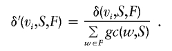 |
In other words, the normalized genetic contribution density δ′(vi,S,F) up to founder vi is computed on founders from F ranked by decreasing values of genetic contribution gc(vi,S) and is normalized over their total genetic contribution. In this context, density can also be interpreted as an incremental genetic contribution computation, when founders are incrementally considered in decreasing order of genetic contribution. In the case of equal genetic contribution, the identifiers of the founders are arbitrarily considered for ordering purposes.
The average normalized genetic contribution density is
 |
where n is the number of founders.
In the hypothetical case of uniform genetic contribution from n founders—that is, when each founder’s contribution is 1/n—the genetic contribution density δ′U is
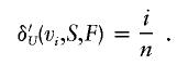 |
The average normalized uniform genetic contribution density is
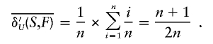 |
The founder effect fe can be quantitatively measured by the following equation:
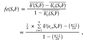 |
where, again, V is the total population, P is the power set, and n is the number of founders in set F. The founder-effect measure fe(S,F) computes the difference between the average genetic contribution density,  , and the hypothetical uniform contribution density,
  , for the same number of founders and normalizes it over the range of this difference—that is, the range between 1, for single-founder contribution, and
  , for uniform contribution.
Electronic-Database Information
The URL for data presented herein is as follows:
References
- Allison DB, Neale MC, Zannolli R, Schork NJ, Amos CI, Blangero J (1999) Testing the robustness of the likelihood-ratio test in a variance-component quantitative-trait loci–mapping procedure. Am J Hum Genet 65:531–544 [DOI] [PMC free article] [PubMed] [Google Scholar]
- Atzmon G, Schechter C, Greiner W, Davidson D, Rennert G, Barzilai N (2004) Clinical phenotype of families with longevity. J Am Geriatr Soc 52:274–277 [DOI] [PubMed] [Google Scholar]
- Beaumont MA, Rannala B (2004) The Bayesian revolution in genetics. Nat Rev Genet 5:251–261 [DOI] [PubMed] [Google Scholar]
- Blangero J, Williams JT, Almasy L (2001) Variance component methods for detecting complex trait loci. Adv Genet 42:151–181 [DOI] [PubMed] [Google Scholar]
- Bouchard G, Roy R, Casgrain B, Hubert M (1989) [Population files and database management: the BALSAC database and the INGRES/INGRID system]. Hist Mes 4:39–57 [PubMed] [Google Scholar]
- Burt VL, Culter JA, Higgins M, Horan MJ, Labarthe D, Whelton P, Brown C, Roccella EJ (1995) Trends in the prevalence, awareness, treatment, and control of hypertension in the adult US population: data from the health examination surveys, 1960 to 1991. Hypertension 26:60–69 [DOI] [PubMed] [Google Scholar]
- Caulfield M, Munroe P, Pembroke J, Samani N, Dominiczak A, Brown M, Benjamin N, Webster J, Ratcliffe P, O’Shea S, Papp J, Taylor E, Dobson R, Knight J, Newhouse S, Hooper J, Lee W, Brain N, Clayton D, Lathrop GM, Farrall M, Connell J (2003) Genome-wide mapping of human loci for essential hypertension. Lancet 361:2118–2123 [DOI] [PubMed] [Google Scholar]
- Daly MJ, Rioux JD, Schaffner SF, Hudson TJ, Lander ES (2001) High-resolution haplotype structure in the human genome. Nat Genet 29:229–232 [DOI] [PubMed] [Google Scholar]
- Daw EW, Heath SC, Wijsman EM (1999) Multipoint oligogenic analysis of age-at-onset data with applications to Alzheimer disease pedigrees. Am J Hum Genet 64:839–851 [DOI] [PMC free article] [PubMed] [Google Scholar]
- Doris PA (2002) Hypertension genetics, single nucleotide polymorphisms, and the common disease: common variant hypothesis. Hypertension 39:323–331 [DOI] [PubMed] [Google Scholar]
- Ezzati M, Lopez AD, Rodgers A, Vander HS, Murray CJ (2002) Selected major risk factors and global and regional burden of disease. Lancet 360:1347–1360 [DOI] [PubMed] [Google Scholar]
- Franklin SS (2004) Systolic blood pressure: it’s time to take control. Am J Hypertens 17:49S–54S [DOI] [PubMed] [Google Scholar]
- Franklin SS, Jacobs MJ, Wong ND, L’Italien GJ, Lapuerta P (2001) Predominance of isolated systolic hypertension among middle-aged and elderly US hypertensives: analysis based on National Health and Nutrition Examination Survey (NHANES) III. Hypertension 37:869–874 [DOI] [PubMed] [Google Scholar]
- Gagnon F, Jarvik GP, Motulsky AG, Deeb SS, Brunzell JD, Wijsman EM (2003) Evidence of linkage of HDL level variation to APOC3 in two samples with different ascertainment. Hum Genet 113:522–533 [DOI] [PubMed] [Google Scholar]
- Ghosh S, Majumder PP (2001) Deciphering the genetic architecture of a multivariate phenotype. Adv Genet 42:323–347 [DOI] [PubMed] [Google Scholar]
- Glazier AM, Nadeau JH, Aitman TJ (2002) Finding genes that underlie complex traits. Science 298:2345–2349 [DOI] [PubMed] [Google Scholar]
- Göring HH, Terwilliger JD, Blangero J (2001) Large upward bias in estimation of locus-specific effects from genomewide scans. Am J Hum Genet 69:1357–1369 [DOI] [PMC free article] [PubMed] [Google Scholar]
- Groop L, Orho-Melander M (2001) The dysmetabolic syndrome. J Intern Med 250:105–120 [DOI] [PubMed] [Google Scholar]
- Hamet P, Pausova Z, Adarichev S, Adaricheva K, Tremblay J (1998) Hypertension: genes and environment. J Hypertens 16:397–418 [DOI] [PubMed] [Google Scholar]
- Hanson RL, Ehm MG, Pettitt DJ, Prochazka M, Thompson DB, Timberlake D, Foroud T, Kobes S, Baier L, Burns DK, Almasy L, Blangero J, Garvey WT, Bennett PH, Knowler WC (1998) Autosomal genomic scan for loci linked to type II diabetes mellitus and body-mass index in Pima Indians. Am J Hum Genet 63:1130–1138 [DOI] [PMC free article] [PubMed] [Google Scholar]
- Hauser ER, Crossman DC, Granger CB, Haines JL, Jones CJ, Mooser V, McAdam B, et al (2004a) A genomewide scan for early-onset coronary artery disease in 438 families: the GENECARD Study. Am J Hum Genet 75:436–447 [DOI] [PMC free article] [PubMed] [Google Scholar]
- Hauser ER, Watanabe RM, Duren WL, Bass MP, Langefeld CD, Boehnke M (2004b) Ordered subset analysis in genetic linkage mapping of complex traits. Genet Epidemiol 27:53–63 [DOI] [PubMed] [Google Scholar]
- Heath SC (1997) Markov chain Monte Carlo segregation and linkage analysis for oligogenic models. Am J Hum Genet 61:748–760 [DOI] [PMC free article] [PubMed] [Google Scholar]
- Helgadottir A, Manolescu A, Thorleifsson G, Gretarsdottir S, Jonsdottir H, Thorsteinsdottir U, Samani NJ, et al (2004) The gene encoding 5-lipoxygenase activating protein confers risk of myocardial infarction and stroke. Nat Genet 36:233–239 [DOI] [PubMed] [Google Scholar]
- Heyer E, Tremblay M (1995) Variability of the genetic contribution of Quebec population founders associated to some deleterious genes. Am J Hum Genet 56:970–978 [PMC free article] [PubMed] [Google Scholar]
- Jacobs KB, Gray-McGuire C, Cartier KC, Elston RC (2003) Genome-wide linkage scan for genes affecting longitudinal trends in systolic blood pressure. BMC Genet 4:S82 [DOI] [PMC free article] [PubMed] [Google Scholar]
- James K, Weitzel LR, Engelman CD, Zerbe G, Norris JM (2003) Genome scan linkage results for longitudinal systolic blood pressure phenotypes in subjects from the Framington Heart Study. BMC Genet 4:S83 [DOI] [PMC free article] [PubMed] [Google Scholar]
- Jeunemaître X, Soubrier F, Kotelevtsev YV, Lifton RP, Williams CS, Charru A, Hunt SC, Hopkins PN, Williams RR, Lalouel JM, Corvol P (1992) Molecular basis of human hypertension: role of angiotensinogen. Cell 71:169–180 [DOI] [PubMed] [Google Scholar]
- Joffres MR, Hamet P, Maclean DR, L’Italien GJ, Fodor G (2001) Distribution of blood pressure and hypertension in Canada and the United States. Am J Hypertens 14:1099–1105 [DOI] [PubMed] [Google Scholar]
- Kotchen TA, Broeckel U, Grim CE, Hamet P, Jacob H, Kaldunski ML, Kotchen JM, Schork NJ, Tonellato PJ, Cowley AW Jr (2002) Identification of hypertension-related QTLs in African American sib pairs. Hypertension 40:634–639 [DOI] [PubMed] [Google Scholar]
- Kotchen TA, Kotchen JM, Grim CE, George V, Kaldunski ML, Cowley AW, Hamet P, Chelius TH (2000) Genetic determinants of hypertension: identification of candidate phenotypes. Hypertension 36:7–13 [DOI] [PubMed] [Google Scholar]
- Labuda M, Labuda D, Korab-Laskowska M, Cole DEC, Zietkiewicz E, Weissenbach J, Popowska E, Pronicka E, Root AW, Glorieux FH (1996) Linkage disequilibrium analysis in young populations: pseudo–vitamin D–deficiency rickets and the founder effect in French Canadians. Am J Hum Genet 59:633–643 [PMC free article] [PubMed] [Google Scholar]
- Labuda D, Zietkiewicz E, Labuda M (1997) The genetic clock and the age of the founder effect in growing populations: a lesson from French Canadians and Ashkenazim. Am J Hum Genet 61:768–771 [PMC free article] [PubMed] [Google Scholar]
- Lander ES, Schork NJ (1994) Genetic dissection of complex traits. Science 265:2037–2048 [DOI] [PubMed] [Google Scholar]
- Langefeld CD, Wagenknecht LE, Rotter JI, Williams AH, Hokanson JE, Saad MF, Bowden DW, Haffner S, Norris JM, Rich SS, Mitchell BD (2004) Linkage of the metabolic syndrome to 1q23-q31 in Hispanic families: the Insulin Resistance Atherosclerosis Study Family Study. Diabetes 53:1170–1174 [DOI] [PubMed] [Google Scholar]
- Lifton RP, Gharavi AG, Geller DS (2001) Molecular mechanisms of human hypertension. Cell 104:545–556 [DOI] [PubMed] [Google Scholar]
- Loos RJ, Katzmarzyk PT, Rao DC, Rice T, Leon AS, Skinner JS, Wilmore JH, Rankinen T, Bouchard C (2003) Genome-wide linkage scan for the metabolic syndrome in the HERITAGE Family Study. J Clin Endocrinol Metab 88:5935–5943 [DOI] [PubMed] [Google Scholar]
- McAdoo WG, Weinberger MH, Miller JZ, Fineberg NS, Grim CE (1990) Race and gender influence hemodynamic responses to psychological and physical stimuli. J Hypertens 8:961–967 [DOI] [PubMed] [Google Scholar]
- Newman DL, Abney M, Dytch H, Parry R, McPeek MS, Ober C (2003) Major loci influencing serum triglyceride levels on 2q14 and 9p21 localized by homozygosity-by-descent mapping in a large Hutterite pedigree. Hum Mol Genet 12:137–144 [DOI] [PubMed] [Google Scholar]
- O’Brien E, Kerber RA, Jorde LB, Rogers AR (1994) Founder effect: assessment of variation in genetic contributions among founders. Hum Biol 66:185–204 [PubMed] [Google Scholar]
- Pausova Z, Deslauriers B, Gaudet D, Tremblay J, Kotchen TA, Larochelle P, Cowley AW, Hamet P (2000) Role of tumor necrosis factor-α gene locus in obesity and obesity-associated hypertension in French Canadians. Hypertension 36:14–19 [DOI] [PubMed] [Google Scholar]
- Pausova Z, Gossard F, Gaudet D, Tremblay J, Kotchen TA, Cowley AW, Hamet P (2001) Heritability estimates of obesity measures in siblings with and without hypertension. Hypertension 38:41–47 [DOI] [PubMed] [Google Scholar]
- Pausova Z, Jomphe M, Houde L, Vezina H, Orlov SN, Gossard F, Gaudet D, Tremblay J, Kotchen TA, Cowley AW, Bouchard G, Hamet P (2002) A genealogical study of essential hypertension with and without obesity in French Canadians. Obes Res 10:463–470 [DOI] [PubMed] [Google Scholar]
- Pausova Z, Tremblay J, Hamet P (1999) Gene-environment interactions in hypertension. Curr Hypertens Rep 1:42–50 [DOI] [PubMed] [Google Scholar]
- Peltonen L, Palotie A, Lange K (2000) Use of population isolates for mapping complex traits. Nat Rev Genet 1:182–190 [DOI] [PubMed] [Google Scholar]
- Perola M, Kainulainen K, Pajukanta P, Terwilliger JD, Hiekkalinna T, Ellonen P, Kaprio J, Koskenvuo M, Kontula K, Peltonen L (2000) Genome-wide scan of predisposing loci for increased diastolic blood pressure in Finnish siblings. J Hypertens 18:1579–1585 [DOI] [PubMed] [Google Scholar]
- Province MA, Kardia SL, Ranade K, Rao DC, Thiel BA, Cooper RS, Risch N, Turner ST, Cox DR, Hunt SC, Weder AB, Boerwinkle E (2003) A meta-analysis of genome-wide linkage scans for hypertension: the National Heart, Lung and Blood Institute Family Blood Pressure Program. Am J Hypertens 16:144–147 [DOI] [PubMed] [Google Scholar]
- Ranade K, Hinds D, Hsiung CA, Chuang LM, Chang MS, Chen YT, Pesich R, Hebert J, Chen YD, Dzau V, Olshen R, Curb D, Botstein D, Cox DR, Risch N (2003) A genome scan for hypertension susceptibility loci in populations of Chinese and Japanese origins. Am J Hypertens 16:158–162 [DOI] [PubMed] [Google Scholar]
- Reaven GM (2004) Insulin resistance, cardiovascular disease, and the metabolic syndrome: how well do the emperor’s clothes fit? Diabetes Care 27:1011–1012 [DOI] [PubMed] [Google Scholar]
- Rice T, Rankinen T, Province MA, Chagnon YC, Perusse L, Borecki IB, Bouchard C, Rao DC (2000) Genome-wide linkage analysis of systolic and diastolic blood pressure: the Quebec Family Study. Circulation 102:1956–1963 [DOI] [PubMed] [Google Scholar]
- Rioux JD, Stone VA, Daly MJ, Cargill M, Green T, Nguyen H, Nutman T, Zimmerman PA, Tucker MA, Hudson T, Goldstein AM, Lander E, Lin AY (1998) Familial eosinophilia maps to the cytokine gene cluster on human chromosomal region 5q31-q33. Am J Hum Genet 63:1086–1094 [DOI] [PMC free article] [PubMed] [Google Scholar]
- Samani NJ (2003) Genome scans for hypertension and blood pressure regulation. Am J Hypertens 16:167–171 [DOI] [PubMed] [Google Scholar]
- Scriver CR (2001) Human genetics: lessons from Quebec populations. Annu Rev Genomics Hum Genet 2:69–101 [DOI] [PubMed] [Google Scholar]
- Siegmund D (2002) Upward bias in estimation of genetic effects. Am J Hum Genet 71:1183–1188 [DOI] [PMC free article] [PubMed] [Google Scholar]
- Steil GM, Volund A, Kahn SE, Bergman RN (1993) Reduced sample number for calculation of insulin sensitivity and glucose effectiveness from the minimal model. Diabetes 42:250–256 [DOI] [PubMed] [Google Scholar]
- Stein CM, Song Y, Elston RC, Jun G, Tiwari HK, Iyengar SK (2003) Structural equation model-based genome scan for the metabolic syndrome. BMC Genet 4:S99 [DOI] [PMC free article] [PubMed] [Google Scholar]
- Stoll M, Cowley AW Jr, Tonellato PJ, Greene AS, Kaldunski ML, Roman RJ, Dumas P, Schork NJ, Wang Z, Jacob HJ (2001) A genomic-systems biology map for cardiovascular function. Science 294:1723–1726 [DOI] [PubMed] [Google Scholar]
- Tang W, Miller MB, Rich SS, North KE, Pankow JS, Borecki IB, Myers RH, Hopkins PN, Leppert M, Arnett DK (2003) Linkage analysis of a composite factor for the multiple metabolic syndrome: the National Heart, Lung, and Blood Institute Family Heart Study. Diabetes 52:2840–2847 [DOI] [PubMed] [Google Scholar]
- Turnbull F, Blood Pressure Lowering Treatment Trialists’ Collaboration (2003) Effects of different blood-pressure-lowering regimens on major cardiovascular events: results of prospectively-designed overviews of randomised trials. Lancet 362:1527–1535 [DOI] [PubMed] [Google Scholar]
- Ueno T, Tremblay J, Kunes J, Zicha J, Dobesova Z, Pausova Z, Deng AY, Sun YL, Jacob HJ, Hamet P (2004) Rat model of familial combined hyperlipidemia as a result of comparative mapping. Physiol Genomics 17:38–47 [DOI] [PubMed] [Google Scholar]
- von Wowern F, Bengtsson K, Lindgren CM, Orho-Melander M, Fyhrquist F, Lindblad U, Rastam L, Forsblom C, Kanninen T, Almgren P, Burri P, Katzman P, Groop L, Hulthen UL, Melander O (2003) A genome wide scan for early onset primary hypertension in Scandinavians. Hum Mol Genet 12:2077–2081 [DOI] [PubMed] [Google Scholar]
- Wijsman EM (2002) Joint linkage and segregation analysis using Markov chain Monte Carlo methods. Methods Mol Biol 195:139–161 [DOI] [PubMed] [Google Scholar]
- Woolley N, Holopainen P, Ollikainen V, Mustalahti K, Maki M, Kere J, Partanen J (2002) A new locus for coeliac disease mapped to chromosome 15 in a population isolate. Hum Genet 111:40–45 [DOI] [PubMed] [Google Scholar]