Mining frequent patterns in protein structures: a study of protease families

Abstract

Motivation

Analysis of protein sequence and structure databases usually reveal frequent patterns (FP) associated with biological function. Data mining techniques generally consider the physicochemical and structural properties of amino acids and their microenvironment in the folded structures. Dynamics is not usually considered, although proteins are not static, and their function relates to conformational mobility in many cases.

Results

This work describes a novel unsupervised learning approach to discover FPs in the protein families, based on biochemical, geometric and dynamic features. Without any prior knowledge of functional motifs, the method discovers the FPs for each type of amino acid and identifies the conserved residues in three protease subfamilies; chymotrypsin and subtilisin subfamilies of serine proteases and papain subfamily of cysteine proteases. The catalytic triad residues are distinguished by their strong spatial coupling (high interconnectivity) to other conserved residues. Although the spatial arrangements of the catalytic residues in the two subfamilies of serine proteases are similar, their FPs are found to be quite different. The present approach appears to be a promising tool for detecting functional patterns in rapidly growing structure databases and providing insights in to the relationship among protein structure, dynamics and function.

1 INTRODUCTION

Elucidation of a protein’s three-dimensional (3D) structure is viewed as a major step in understanding the molecular basis of its biological function. Knowledge of structure may not be sufficient, however, for understanding the mechanism of function, because biological function often depends on conformational dynamics. Usually, the protein function is associated with particular sequence or structure motifs, and the identification of functional patterns and their role in the overall dynamics of the protein requires additional data and analysis. With the exponential growth in the number of experimentally determined structures in the Protein Data Bank (PDB) (Berman et al., 2000), a wealth of computational methods, usually based on sequence comparisons, have been developed to examine or extract such patterns, while structural dynamics has not been systematically invoked. One can utilize pattern recognition approaches using prior biological knowledge, or adopt pattern discovery methods to find statistically significant patterns that can be tested and verified experimentally.

A small number of residues are usually reported to be directly involved in protein function. This suggests that there are strong correlations between function and microenvironment. Microenvironment refers to the local structure assumed by residues close in space, but not necessarily contiguous along the sequence. Protein function is however a collective property of the structure, and it is conceivable that the global protein dynamics is coupled with the local structure near the active site.

A catalytic residue dataset (Bartlett et al., 2002) was built by manually extracting information from primary sources in the literature. A thorough analysis, in terms of secondary structure, solvent accessibility, flexibility, conservation, quaternary structure and function, has been performed on the residues directly involved in catalysis in 178 enzyme active sites. This work provided a good understanding of the molecular features that affect catalytic function and, in particular, the importance of flexibility. However, it is not designed to retrieve information automatically, or to discover new frequent patterns (FPs).

Several web-based databases to search similar substructures are freely available in the public domain. PROCAT (Wallace et al., 1997) uses a geometric hashing algorithm to build and search 3D enzyme active site templates from conserved geometry. WEBFEATURE (Bagley and Altman, 1995; Liang et al., 2003) applies a Bayesian supervised learning algorithm for a succinct characterization of the site microenvironment, expressed in terms of a set of biochemical properties. However, the results are sensitive to assumptions about background distributions and training sites chosen. The PINTS (Patterns in non-homologous tertiary structures) server (Stark and Russell, 2003) allows for searches of a reasonably large number of predefined structure and function motifs in three different ways: (1) protein versus pattern database (2) pattern versus protein database and (3) pairwise comparison of proteins. This work is significant as it detects similarities in the spatial arrangement of side chains among protein structures without any prior knowledge of the active or binding site (Russell, 1998). It also develops a statistics to calculate the significance of root-mean-square deviation (RMSD) between spatial positions of equivalent amino acids after optimal superimposition of matching structural patterns (Stark and Russell, 2003). However, the algorithm is developed to find local patterns (radius <7.5 Å) in non-homologous proteins, exclusively, and suffers if two similar proteins are compared. It excludes amino acids with side chains containing only H and C atoms (Ala, Phe, Gly, Ile, Leu, Pro and Val) that are not specific enough to efficiently discriminate between correct and false matches.

Two other unsupervised methods have proved to conduct successful discovery of novel sequence–structure pattern. I-site (Bystroff and Baker, 1998) is a library of short sequence patterns that strongly correlate with 3D structural elements of protein. It provides a new methodology for local structure prediction. TRILOGY (Bradley et al., 2002) treats both sequence and structure component as patterns, which are identified and extended simultaneously during the search process. Thousands of significant sequence–structure patterns were discovered in this work. However, patterns of structurally conserved residues are not necessarily adjacent in the protein sequence and can occur in any order, such as the trypsin-like catalytic triad. Patterns that lack sequence–pattern component will not be detected by these algorithms.

In this work, a novel unsupervised learning approach is proposed to discover FPs in protein (sub)families. In addition to sequence and structure similarities, structural dynamics are considered. These patterns are thus characterized in terms of their dynamics, biochemistry and geometry in the microenvironment. Without any sequence alignment, structurally conserved residues whose sequence and order are not necessarily well maintained can be identified. Experiments indicate different patterns in the microenvironment at the catalytic triad of the examined three protease subfamilies, which are correctly distinguished in the detected patterns.

2 METHODS

An overview of the proposed method is presented in Figure 1. A set of proteins belonging to a given family is selected as the training dataset. Features are extracted from all the amino acids in this dataset. Each amino acid corresponds to one entry, represented by the amino acid sequence index and the extracted features. These entries are organized into 20 groups by amino acid type. The Apriori algorithm is applied to each group to find FPs that correspond to different amino acids. All the residues exhibiting conserved features are identified by an iterative search algorithm, and these residues are further ranked by the level of their interconnectivity in the 3D structure.

Fig. 1.

Overview of the proposed method.

2.1 Dataset

Two classes of enzymes, serine proteases and cysteine proteases are analyzed here. Serine proteases typically have a His–Asp–Ser catalytic triad at the active site. These three residues, which occur far apart along the amino acid sequence, are grouped together in the 3D structure to form the specific conformation at the active site of the enzyme. Cysteine proteases catalytic residues also have similar clustering properties, the triad being often comprised of Cys, His and Asn. Conserved geometric and dynamic patterns presumably occur in the microenvironment of the catalytic triad, in line with the specific function of hydrolytic cleavage of the appropriate bond in the substrate. The proposed unsupervised learning algorithm will detect these patterns.

The Enzyme Classification Database (Bairoch, 1993) contains 780 PDB entries corresponding to the serine proteases class E.C.3.4.21, and 122 entries corresponding to the cysteine proteases class E.C.3.4.22 (as of 28 March 2003). These enzymes are classified into evolutionary subfamilies (Rawlings and Barrett, 1993). In this work, two largest subfamilies, S1-Chymotrypsin (S1) and S8-Subtilisin (S8), of serine proteases and the largest subfamily, C1-Papain (C1), of cysteine proteases are examined. To reduce structural redundancy, 90% sequence identity is used to select representative chains from the PDB by PDB-REPRDB (Noguchi and Akiyama, 2003), which yields 79, 7 and 6 representative proteins in S1, S8 and C1 subfamilies, respectively. In FEATURE (Bagley and Altman, 1995), six proteins, namely 1arb, 1gct, 1sgt, 1ton, 3est and 4ptp, were examined to characterize the microenvironment of catalytic triads. The same proteins are included in our analysis of S1 subfamily, except for 1arb that belongs to another (S5-lysyl endopeptidase) subfamily; all representative proteins of the S8 and C1 subfamilies are included in our analysis (Table 1).

Table 1.

Proteins examined in the present study

S1 Chymotrypsin
Gamma-chymotrypsin A, 1gct, 3.4.21.1	240	H57, D102, S195
Trypsin, 1sgt, 3.4.21.4	223	H57, D102, S195
Tonin, 1ton, 3.4.21.35	227	H57, D102, S195
Native elastase, 3est, 3.4.21.36	240	H57, D102, S195
Beta trypsin, 4ptp, 3.4.21.4	223	H57, D102, S195
S8 Subtilisin
Subt. carlsberg complex, 2sec, 3.4.21.62	338	D32, H64, S221
Complex of subt. bpn’, 1lw6, 3.4.21.62	344	D32, H64, S221
Subtilisin dy in complex, 1bh6, 3.4.21.62	274	D32, H64, S221
Savinase, 1svn, 3.4.21.62	269	D32, H64, S221
Mesentericopeptidase, 1mee, 3.4.21.62	339	D32, H64, S221
Proteinase k, 1ic6, 3.4.21.64	279	D39, H72, S224
Thermitase, 1thm, 3.4.21.66	279	D38, H74, S225
C1 Papain
Cathepsin b, 1huc, 3.4.22.1	252	C29, H199, N219
Cathepsin b, 1the, 3.4.22.1	253	C29, H199, N219
Procathepsin b, 3pbh, 3.4.22.1	317	C29, H199, N219
Cathepsin l, 1icf, 3.4.22.15	217	C25, H163, N187
Papain cys-25, 1ppn, 3.4.22.2	212	C25, H159, N175
Protease omega, 1ppo, 3.4.22.30	216	C25, H159, N179

2.2 Feature extraction

The microenvironment near each residue is defined as a spherical region of 7.0 Å radius centered about its C^α-atom. Each amino acid is characterized in terms of its dynamic features (see below), and the biochemical and geometric features of the residues in its microenvironment.

2.2.1 Dynamic features: Gaussian network model

The Gaussian network model (GNM) (Bahar et al., 1997, 1998), an elastic network model for describing the equilibrium dynamics of proteins, is used for characterizing the dynamics features. In the GNM, the α-carbons (C^α) form the network nodes, and the nodes located within an interaction cut-off distance of 7.0 Å are connected via uniform elastic springs. The network connectivity is described by a Kirchhoff matrix Γ (Bahar et al., 1997). The element Γ_ij = 1 if residues i and j are connected, and zero otherwise; and Γ_ii = −z_i, where z_i, is the number of connections at node i (also called contact number CN; see below). The diagonal terms of Γ⁻¹ scale with mean-square fluctuations of residues, and the off-diagonal terms scale with the cross-correlations. Application to more than 100 proteins showed that the GNM predictions agree well with experimental data (Kundu et al., 2002).

A major utility of the GNM is the rapid assessment of collective modes of motions (Bahar et al., 1999). The i-th eigenvector of Γ represents the i-th mode shape (i.e. distribution of residue mobilities), the frequency of which scales with the i-th eigenvalue. The slow modes have been shown in numerous applications to drive cooperative motions (i.e. domain movements, hinge-bending motions, etc.) relevant to biological function. See for example, the application to hemoglobin T → R2 transition (Xu et al., 2003) and the references cited therein. Here, the slowest two modes, referred to as slow mode 1 (S1) and slow mode 2 (S2), are examined, and the mobilities of individual residues in these modes are mapped into a scale of 10 levels, varying from 0 (rigid) to 9 (very mobile). The residues subject to the smallest and largest motions in S1, for example, are assigned the attributes S1-0 and S1-9, respectively.

Another structural property that has been confirmed in numerous studies to have a strong impact on equilibrium dynamics is the CN, which is defined as the number of amino acids (or α-carbons) that coordinate the central amino acid within a first interaction shell of 7.0 Å. Examination of PDB structures shows that the CNs vary over a broad range (2 ≤ CN ≤ 16). The lower limit refers to the sequential neighbors at fully extended and solvent-exposed regions, and the upper limit refers to highly packed core regions. Accordingly, the observed CNs were mapped here into four discrete levels CN-1, CN-2, CN-3, CN-4, corresponding to the respective ranges 2 ≤ CN ≤ 4, 5 ≤ CN ≤ 8, 9 ≤ CN ≤ 12 and 13 ≤ CN ≤ 16.

In a strict sense, mobilities and contact numbers are not independent, the regions subject to high CN being constrained in space. However, mobilities contain the additional effect of distribution of contacts characteristic of the particular protein architecture, and our results support the inclusion of both attributes for detecting FPs.

2.2.2 Biochemical features: amino acid type and property

The amino acid classification is based here on both the specific amino acid identity (Ala, Val, etc.) and the side chain chemical features or functional groups (Koolman and Rohm, 1996), defined as aliphatic (ALI): Gly, Ala, Val, Leu and Ile; S-containing (SULFUR): Cys and Met; aromatic (ARO): Phe, Tyr and Trp; neutral/polar (NEUTR): Ser, Thr, Asn and Gln; acidic (ACID): Asp and Glu; Basic (BASIC): Lys, Arg and His; and imino acid (IMI): Pro. Thus, a lysine residue, for example, is assigned two features, LYS and BASIC. The use of features associated with taxonomy information allows for ‘mining multiple level association rules’ (Han and Fu, 1995), and provides more flexibility, since it would be too restrictive to consider amino acid types, only, without side chains properties, and it would not be specific enough to consider side chains properties only.

2.2.3 Geometric features: 3D reference frame

A 3D reference frame (Pennec and Ayache, 1994) is ascribed to each residue, using the three backbone atoms N, C^α and C′ (carbonyl C). These three atoms form a frame (a point and a trihedron; Fig. 2A) that uniquely defines the position and orientation of the residue in the 3D space. The origin of the reference frame coincides with the C^α atom, and the three directional vectors e₁, e₂ and e₃ are defined in Figure 2B. The microenvironment is divided into eight quadrants using (±e₁, ±e₂, ±e₃), numbered from Q1 to Q8 (Fig. 2C). All the biochemical features, extracted for the residues in the microenvironment are expressed with reference to this quadrant information, the residue positions being identified by their C^α-atom coordinates. The combined biochemical–geometric features were found to yield a sufficiently discriminative description of the structural and functional properties in the microenvironment.

Fig. 2.

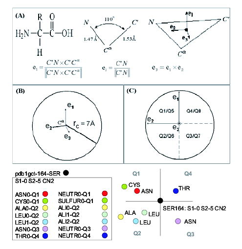
Feature extraction methodology. (A) Definition of residue-centered reference-frame. (B) Examination of microenvironment, and the type and identity of residues in the geometric subspaces Q1–Q8 and (C) the results for Ser-164, in S1 subfamily.

2.2.4 A feature extraction example: 1gct-Ser-164

Let us consider the Ser-164 of the PDB file 1gct as an illustrative example for feature extraction (Fig. 2). Ser-164 is found by the GNM to have minimal fluctuations/mobilities in the slow mode 1 (S1-0) and a moderate mobility (level 2) in slow mode 2 (S2-5). It has seven neighbors in its microenvironment, so its contact number falls into the range 2 (CN2). The seven neighbors consist of one Asn and one Cys in Q1 (note that the index starts from 0), one Ala and two Leu in Q2, one Asn in Q3 and one Thr in Q4. According to the amino acid classification outlined in Section 2.2.2, the microenvironment contains a neutral and a sulfur-containing residue in Q1, three aliphatic residues in Q2, a neutral residue in Q3 and in Q4, as summarized in Figure 2.

2.3 FP discovery—Apriori algorithm

An implementation of the Apriori algorithm (Borgelt and Kruse, 2002; Agrawal et al., 1993) is used for the induction of association rules. Figure 3 illustrates how this method works. Let us suppose that we are interested in the characterization of the histidine residues in a given protein family. Let us assume that the family is comprised of two proteins, PDB1arb and PDB4ptp. PDB1arb has two histidines, His-57 and His-149, and PDB4ptp has one, His-57.

Fig. 3.

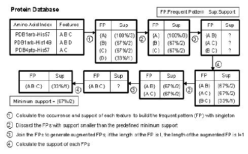
An illustrative example of a priori algorithm.

The geometric, biochemical and dynamic features described above are extracted for each of the three histidines of all proteins in the database. For illustrative purposes, let us denote these features as {A}, {B}, {C} and {D}. The number of occurrences of each feature is counted first to determine the initial FPs with singleton (process 1 in Fig. 3). A FP is often evaluated by its absolute or relative support. The absolute support is the number of times an FP is observed in the database. The relative support is the percentage of absolute support in the database. Here, {B} occurs 2 times in 3 tested histidines, and therefore has a relative support of 67% and an absolute support of 2, which is concisely designated as 67%/2. Typically, the larger the support, the more significant the FP is. The minimum support is suitably set to meet the need of different database users. Relatively low minimum support may include less important FPs and increase the computational complexity. In this example, the minimum support is set to be 67%/2.

The length of the initial singleton FP is one since it has only one feature, and its length will be augmented by one at each iterative step, by selecting the FPs that satisfy the minimum support requirement (process 2). The remaining FPs are combined together to generate the augmented FPs (process 3). The supports of the augmented FPs are then calculated (process 4). The steps 2–4 are repeated until the FP with maximum length is reached. In Figure 3, the longest FP is {ABC}, with support 33%/1. Alternatively, the shorter FPs {AB} and {AC} with larger support (67%2) could have been identified. There is usually a compromise between FP length and its support, and the optimal FP length/support varies depending on the specific questions addressed.

2.4 Identification of conserved residues

In the application of the Apriori algorithm to proteins, first the FPs with maximum length were discovered in the neighborhood of each type of amino acid. The FP was considered to be a ‘conserved FP’ provided that it occurred at least once in each protein belonging to the examined subfamily. Those residues participating in conserved FPs were identified as ‘conserved residues’. Next, the conserved residues are removed from the original dataset, and the Apriori algorithm is applied again to the modified dataset. Other FPs with shorter length and the corresponding conserved residues are identified. This procedure is performed iteratively until the longest FP that is not ‘conserved’ is hit. All the conserved patterns of 20 types of amino acids were identified by this iterative search for each family.

2.5 Rank of conserved residues

Once the conserved residues are identified by the Apriori algorithm, a ranking method is needed to distinguish the catalytic residues. It is assumed that the catalytic residues are optimally coupled with other conserved residues to achieve the highest cooperativity. Coupling in 3D is expressed as the number of contacts made with the conserved residues. To this aim, each conserved amino acid is represented by its side chain centroid (except for Gly where C^α is used); the centroids separated by <7.0 Å are connected to form a network of conserved residues; and the number of connections at each junction (centroid) is counted. The amino acids that show the lowest interconnectivity (smallest number of connected neighbors) are removed from the list of considered residues. The connectivity of the network formed by the remaining conserved residues is examined again, and the residue with the lowest rank is removed, and so on. This procedure is repeated until the ‘core’ residues, which are all interconnected, are reached. The ‘core’ residues are assigned the score zero, and the others are scored according to the number of iterations required to reach the ‘core’ residues. All the conserved residues were thus scored for each protein in the training dataset, and an average score 〈 s 〉 over all family members was calculated for each conserved residue. A cut-off threshold for the score was assessed from the receiver operating characteristic (ROC) curve (see Section 3.5).

3 RESULTS AND DISCUSSION

3.1 Identification of conserved residues

Let us consider the serine residues in the serine protease family as an example. Information for a set of 111 serine residues is extracted from the 5 proteins in S1, and for a set of 250 serine residues from the 7 proteins in S8. Since each of these proteins contains one His–Asp–Ser catalytic triad, the minimum support is then set to be the number of proteins divided by the total number of a certain kind of amino acid in this dataset, i.e. the minimum support for serine residues is 5/111 (or 4.5%) for S1 and 7/250 (or 2.8%) for S8. The Apriori algorithm described above is then applied to each set of entries to identify the conserved serines. The analysis yields two serine residues in the S1-Chymotrypsin subfamily (Ser-195 and Ser-214 using the sequence index of 1gct), and four (Ser-221, Ser-125, Ser-190 and Ser-207 in 1svn) in the S8-subtilisin family (Table 2).

Table 2.

Conserved residues identified by Apriori algorithm^a

S1-Chymotrypsin: representative protein: 1gct
HIS	ASP	SER	ALA	CYS	GLY	TRP	ILE	Others
57(8)	194(13)	195(15)	55(16)	42(13)	196(19)	141(11)	212(8)	N/A
	102(11)	214(11)	183(11)	191(13)	44(15)
			56(10)	58(9)	142(14)
				182(9)	140(14)
					43(14)
					193(13)
					197(13)
					211(7)
S8-Subtilisin: representative protein: 1svn
HIS	ASP	SER	ALA	ASN	LEU	MET	PRO	THR	VAL	PHE	Others
67(15)	32(14)	221(15)	223(20)	155(9)	96(13)	222(18)	225(14)	220(17)	177(14)	189(4)	N/A
226(14)	181(5)	125(11)	228(19)		233(11)		201(8)	66(16)
64(9)		190(8)			126(9)
		207(7)
C1-Papain: representative protein: 1huc
HIS	CYS	ASN	ALA	GLN	GLY	TRP	ILE	LEU	PHE	PRO	SER	TYR	Others
199(4)	29(18)	219(12)	31(14)	23(15)	229(11)	30(12)	201(6)	216(8)	32(14)	76(7)	28(18)	146(7)	N/A
	26(9)		34(11)		27(11)	221(12)	203(6)				220(11)	214(7)
	71(9)				73(9)						152(8)	94(6)
	62(6)				70(9)

^aThe residue numbers along the sequence of the representative chain of each subfamily are listed. The numbers in parantheses show the lengths of the corresponding FPs (i.e. the number of attributes conserved among all equivalent residues of the same subfamily members).

The procedure is repeated for all the 20 types of amino acids. The identified conserved residues are listed in Table 2. The entries in the table show the residue number along the sequence (using a representative protein from each family). The numbers in parentheses are the lengths of the FP (i.e. the number of attributes) associated with the particular conserved residue. ‘N/A’ means that no conserved residue was identified. Our results show that, the catalytic residues (highlighted in gray) are all captured by the present FP detection algorithm, while their FPs do not necessarily have the maximum length.

3.2 Frequent pattern discovery

The FPs around the catalytic residues in the two serine protease subfamilies are found to be quite different, as listed in Table 3. The different FPs observed for the same residues in the two families suggest that the microenvironment has a strong effect on the specific catalytic function. Notably, studies that do not consider the amino acid properties in the microenvironment cannot detect the difference in the FPs of the two subfamilies.

Table 3.

Frequent patterns corresponding to catalytic residues

S1
His	S1-0 S2-0 CN-2 ASP0-Q2 ACID0-Q2 ALA0-Q1 ALI0-Q1 ALI0-Q5
Asp	S1-0 S2-0 CN-3 ALI1-Q8 ALI0-Q8 ARO0-Q6 NEUTR0-Q3 SER0-Q3 BASIC0-Q7 HIS0-Q7 ALA0-Q8
Ser	S1-0 S2-0 CN-3 ALI0-Q8 NEUTR0-Q7 SER0-Q7 ACID0-Q5 GLY0-Q8 ALI0-Q4 SULFUR0-Q1 GLY0-Q1 CYS0-Q1 ASP0-Q5 ALA0-Q4 ALI0-Q1
S8
His	CN-2 THR0-Q5 GLY0-Q4 HIS0-Q8 BASIC0-Q8 NEUTR0-Q1 NEUTR0-Q2 ALI0-Q4 NEUTR0-Q5
Asp	CN-3 GLY0-Q4 SER0-Q7 LEU0-Q8 GLY0-Q3 VAL0-Q5 ALI0-Q3 NEUTR0-Q7 ALI0-Q4 NEUTR0-Q4 ALI0-Q2 ALI0-Q1 ALI0-Q8 ALI0-Q5
Ser	S1-0 S2-0 LEU0-Q7 SER0-Q7 THR0-Q5 ALA0-Q6 GLY0-Q1 NEUTR0-Q7 ALA0-Q5 ALI0-Q7 NEUTR0-Q5 NEUTR0-Q8 ALI0-Q1 ALI0-Q6 ALI0-Q5
C1
His	CN-3 ALI0-Q4 ALI0-Q8 ALI0-Q1
Asn	CN-2 S1-0 S2-0 TRP0-Q4 ARO0-Q2 SER0-Q8 GLY0-Q1 ARO0-Q4 BASIC0-Q6 ALI0-Q6 NEUTR0-Q8 ALI0-Q1
Cys	CN-3 S1-0 S2-0 ALA0-Q5 HIS0-Q3 PHE0-Q8 TRP0-Q4 BASIC0-Q3 SER0-Q5 GLN0-Q6 ARO0-Q8 ARO0-Q4 NEUTR0-Q5 GLY0-Q2 NEUTR0-Q6 ALI0-Q2 ALI0-Q4 ALI0-Q5

The dynamic features are indicated in boldface.

Another important factor is the protein dynamics. Many, although not all, catalytic residues have S1 and S2 at the minimum level, i.e. their mobilities are severely restricted. Minima in the slow mode shapes refer to key regions that mediate the global mechanics of the enzyme. Therefore, the catalytic residues tend to occupy key regions from the mechanical point of view, in addition to their chemical role. Finally, the contact numbers are found to be often conserved among the equivalent catalytic residues.

3.3 Comparison with multiple sequence alignments

The multiple sequence alignments (MSA) of the three sets of proteins listed in Table 1 showed that the residues identified by the Apriori algorithm to have conserved FPs in 3D were all conserved in the MSA, but some residues conserved in the MSA did not necessarily have conserved FPs in 3D space. This is consistent with the fact that the conservation of the microenvironment and global dynamics is a more restrictive (and discriminative) feature than sequence conservation. Another observation is that amino acids that sequentially neighbor the catalytic residues tend to be conserved. This was the case near His-57 and Ser-195 of serine proteases and Cys-29 and Asn-221 of cysteine proteases, but not near Asp-102 of serine proteases and His-199 of cysteine proteases.

3.4 Rank of conserved residues

The present unsupervised learning algorithm identified 22, 22 and 26 conserved residues in the S1, S8 and C1 subfamilies, respectively. These residues rank-ordered on the basis of their cooperativity (see Section 2.5) are presented in Table 4, for a representative member (1gct, 1svn and 1huc; columns A, C and E) of each subfamily, along with the average results over the members of each subfamily (columns B, D and F). The numbers after the comma are the scores of the residues. The ‘core’ residues are scored zero. For example, in 1gct (column A), His-57 and Ser-195 are among the six core residues and colored red. The non-catalytic and core residues are colored orange. Although Asp-102 is not at the core, it is still close to the core with score 2. The ribbon diagram of 1gct is shown in Figure 4A. The conserved residues are color-rendered in sticks, and the residues with score higher than 2 are colored gray. The average scores s_avg for the S1-chymotrypsin subfamily are presented in column B. The top ranking residues in a family are colored red (s_avg ≤ 0.5), yellow (0.5 < s_avg ≤ 1.5) and green (1.5 < s_avg ≤ 2.5).

Table 4.

Rank of conserved residues in the three families^a

S1-Chymotrypsin		S8-Subtilisin		C1-Papain
(A)1gct	(B) family	(C) 1svn	(D) family	(E)1huc	(F) family
HIS57, 0	SER195,0	ASP32, 0	SER221, 0.14	HIS199, 0	GLN23, 0.17
SER195, 0	ALA55, 0	HIS64, 0	MET222, 0.29	ASN219, 0	CYS29, 0.33
CYS42, 0	HIS57, 0.2	SER221, 0	HIS64, 0.43	GLN23, 0	SER28, 0.33
ALA55, 0	CYS42, 0.2	SER125, 0	SER125, 1.00	SER220, 0	SER220, 0.83
CYS58, 0	CYS58, 0.2	LEU96, 1	PRO225, 1.43	TRP221, 0	GLY27, 1.00
GLY196, 0	GLY196, 0.2	LEU126, 1	ASP32, 2.00	CYS29, 1	HIS199, 1.67
SER214, 1	SER214, 1.4	MET222, 1	ALA223, 2.14	SER28, 2	CYS26, 2.33
ASP102, 2	ASP102, 1.8	PRO225, 2	THR220, 2.57	GLY27, 3	TRP221, 2.5
GLY43, 3	GLY43, 2.2	ALA223, 3	ASN155, 3.29	CYS26, 4	CYS71, 2.83
ILE212, 3	ILE212, 3.0	THR220, 4	LEU126, 4.14	CYS71, 5	PHE32, 3.17
GLY197, 4	GLY197, 3.0	ASN155, 5	PHE189, 4.29	GLY73, 6	ASN219, 3.33
GLY140, 5	GLY140, 4.0	PHE189, 6	HIS226, 4.71	GLY70, 6	GLY73, 3.83
GLY193, 5	GLY193, 4.0	HIS226, 6	LEU96, 4.85	PHE32, 6	GLY70, 3.83
GLY44, 6	GLY44, 4.4	SER190, 7	SER190, 5.14	ILE201, 7	TRP30, 4.00
ALA56, 6	ASP194, 5.0	PRO201, 7	PRO201, 5.71	TRP30, 7	TYR94, 6.00
GLY142, 6	ALA56, 5.0	HIS67, 8	HIS67, 6.71	GLY229, 8	GLY229. 6.17
ASP194, 6	GLY142, 5.0	VAL177, 9	VAL177, 6.71	ILE203, 8	PRO76, 6.67
CYS191, 7	CYS191, 6.0	SER207, 9	SER207, 7.71	LEU216, 8	LEU216, 7.17
TRP141, 8	TRP141, 6.6	ALA228, 9	ALA228, 7.71	PRO76, 8	ALA31, 7.17
CYS182, 8	CYS182, 7.0	THR66, 10	ASP181, 8.29	TYR214, 8	TYR146, 7.17
ALA183, 8	ALA183, 7.0	ASP181, 10	THR66, 8.71	CYS62, 9	ILE201, 7.33
GLY211, 8	GLY211, 7.0	LEU233, 10	LEU233,17.71	ALA34, 9	ILE203, 7.67
				ALA31, 9	TYR214, 7.67
				SER152, 9	ALA34, 8.17
				TYR146, 9	SER152, 8.33
				TYR94, 9	CYS62, 8.67

^*Catalytic residues are written in italic and bold face. Numbers are the scores defined in Section 2.5.

Fig. 4.

Ribbon diagrams of 1gct (A) and 1svn (B) and the conserved residues identified by the Apriori algorithms. Residues are colored according to their cooperativity scores (Table 4).

The results for S8-Subtilisin family and a representative member (1svn) are shown in columns C and D and Figure 4B. The results for C1-Papain Subtilisin family are shown in columns E and F (the ribbon diagram is not shown due to space limitation). The catalytic residues are all ranked high, although not always the highest, among the conserved residues, which suggest that they are close to the core in 3D space. Interestingly, most of the conserved residues presently detected tend to cluster together in the 3D structure.

3.5 Threshold score and ROC curves

The cutoff score for distinguishing catalytic residues among the set of conserved residues is determined by a ROC plot of [1 − specificity] against sensitivity (Figure 5). Sensitivity provides a measure of the method’s ability to detect all the catalytic residues (true positives, TP), while specificity is a measure of the false positive (FP) rate, given by the ratio TP/(TP+FP). In order to capture all TPs (catalytic residues) while maximizing the specificity, the lowest average score that yields 100% sensitivity needs to be adopted as the threshold score. For the respective S1, S8 and C1 subfamilies, the optimal threshold scores are 1.8, 2.0 and 3.3, based on the scores indicated in red in the columns B, D and F of Table 4. Alternatively, a threshold value common to all examined subfamilies can be defined, which becomes here 3.3, i.e. the maximum of the threshold scores for the individual families. The average ROC curve is shown by the solid line in Figure 5. The curve indicates that on the average 100% sensitivity (i.e. detection of all three catalytic residues) would involve simultaneous identification of two more conserved residues, given that the specificity is ~60%. However, this specificity refers to the pool of conserved residues that are singled out by the Apriori algorithm. If, on the other hand, the method is evaluated with regard to the entire set of N residues, the specificity varies from 96.7 to 99% for the different families.

Fig. 5.

ROC plot—sensitivity versus specificity—for the present algorithm applied to three subfamilies, and the average ROC plot (solid curve). Sensitivity is the fraction of catalytic residues captured with a given threshold (cutoff) score, and specificity is the fraction of catalytic residues (TPs) among all identified (conserved) residues (TPss and FPs). On the average, a sensitivity of 1 is accompanied by a specificity of 0.6, i.e. two additional conserved residues are identified with the three catalytic residues. However, the accuracy of the method is remarkable, given that the five conserved residues (comprising the catalytic triad) are detected amongst N ~ 250 residues.

4 CONCLUSIONS

A novel unsupervised approach to discover biologically meaningful FPs in protein structures is presented in this study. The approach incorporates features associated with collective dynamics (GNM slow mode shapes) as well as the biochemical (amino acid types and physicochemical properties) and geometric (3D coordination directions) features in the microenvironment. Without any knowledge of functional motifs and/or sequence alignments, conserved residues are identified, and the FPs that distinguish these residues are discovered. These conserved residues are further ranked according to their interconnectivity in 3D space. Notably, the catalytic residues emerge among the top-ranking conserved residues, consistent with their optimal packing to engage in cooperative dynamics. The other top-ranking conserved residues could be experimentally examined as elements underlying stability and/or mediating functional communication.

Among the three groups of features considered for detecting frequent patterns, geometric and biochemical features refer to the microenvironment in the 3D structure. Several studies, including the present one, confirm the importance of the microenvironment in defining the functional role of the active residues. A third property—key role in collective dynamics—emerges here as a discriminative feature. While static properties have been invoked in many studies, dynamics is a feature that has not been included in earlier pattern recognition/discovery schema, partly due to the lack of efficient tools for high-throughput characterization of protein dynamics. Recent advances in modeling proteins as elastic networks now permit us to efficiently elucidate the low frequency motions of proteins, and exploit the connection between these motions and the biological function that has been pointed out in numerous studies. Notably, the catalytic residues take part in key regions that control the global dynamics, as evidenced by their minimal mobilities in the slowest modes S1 and S2. This feature suggests that conserved residues are distinguished not only by the unique static properties of their microenvironment, but also by their finely tuned involvement in global dynamics. It also draws attention to the functional coupling between local chemistry and collective mechanics. The set of conserved residues presently identified are indeed engaged in a network of interaction that can be instrumental in inducing allosteric effects or transmitting signals away from the catalytic site.

This approach can be used to discover and annotate all frequent patterns in the protein structure database. In addition, it can help to predict structure and function of uncharacterized proteins, and identify the important amino acids or structural regions. The methodology can be applied to identify novel motifs, folding cores, and/or binding sites that share comparable dynamic features, and assist in better understanding the correlation between structure, dynamics and function.

References

- Agrawal, R., Imielinski, T. and Swami, A. (1993) Mining association rules between sets of items in large databases. In Proceedings of the Conference on Management of Data, Washington DC. pp. 207–216.
- Bagley SC, Altman RB. Characterizing the microenvironment surrounding protein sites. Protein Sci. 1995;4:622–635. doi: 10.1002/pro.5560040404. [DOI] [PMC free article] [PubMed] [Google Scholar]
- Bahar I, Atilgan AR, Erman B. Direct evaluation of thermal fluctuations in protein using a single parameter harmonic potential. Fold Des. 1997;2:173–181. doi: 10.1016/S1359-0278(97)00024-2. [DOI] [PubMed] [Google Scholar]
- Bahar I, Atilgan AR, Demirel MC, Erman B. Vibrational dynamics of proteins: significance of slow and fast modes in relation to function and stability. Phys Rev Lett. 1998;80:2733–2736. [Google Scholar]
- Bahar I, Erman B, Jernigan RL, Atilgan AR, Covell DG. Collective motions of HIV-1 reverse transcriptase. Examination of flexibility and enzyme function. J Mol Biol. 1999;285:1023–1037. doi: 10.1006/jmbi.1998.2371. [DOI] [PubMed] [Google Scholar]
- Bairoch A. The ENZYME data bank. Nucleic Acids Res. 1993;21:3155–3156. doi: 10.1093/nar/21.13.3155. [DOI] [PMC free article] [PubMed] [Google Scholar]
- Bartlett GJ, Porter CT, Borkakoti N, Thornton JM. Analysis of catalytic residues in enzyme active sites. J Mol Biol. 2002;324:105–121. doi: 10.1016/s0022-2836(02)01036-7. [DOI] [PubMed] [Google Scholar]
- Berman HM, Westbrook J, Feng Z, Gilliland G, Bhat TN, Weissig H, Shindyalov IN, Bourne PE. The Protein Data Bank. Nucleic Acids Res. 2000;28:235. doi: 10.1093/nar/28.1.235. [DOI] [PMC free article] [PubMed] [Google Scholar]
- Borgelt, C. and Kruse, R. (2002) Induction of association rules: Apriori implementation. 15th Conference on Computational Statistics (Compstat 2002), Physica Verlag, Heidelberg, Berlin, Germany.
- Bradley P, Kim PS, Berger B. TRILOGY: discovery of sequence–structure patterns across diverse proteins. Proc Natl Acad Sci, USA. 2002;13:8500–8505. doi: 10.1073/pnas.112221999. [DOI] [PMC free article] [PubMed] [Google Scholar]
- Bystroff C, Baker D. Prediction of local structure in proteins using a library of sequence–structure motifs. J Mol Biol. 1998;281:565–577. doi: 10.1006/jmbi.1998.1943. [DOI] [PubMed] [Google Scholar]
- Han, J. and Fu, Y. (1995) Discovery of multiple-level association from large database. Proceedings of 1995 International Conference on Very Large Data Bases (VLDB’95)5, Zurich, Switzerland, September 1995. pp. 420–431.
- Koolman, J. and Rohm, K.H. (1996) Colour Atlas of Biochemistry Thieme, Stuttgart.
- Kundu S, Melton JS, Sorensen DC, Phillips GN. Dynamics of proteins in crystals: comparison of experiment with simple models. Biophys J. 2002;83:723–732. doi: 10.1016/S0006-3495(02)75203-X. [DOI] [PMC free article] [PubMed] [Google Scholar]
- Liang MP, Banatao DR, Klein TE, Brutlag DL, Altman RB. WebFEATURE: an interactive web tool for identifying and visualizing functional sites on macromolecular structures. Nucleic Acids Res. 2003;13:3324–3327. doi: 10.1093/nar/gkg553. [DOI] [PMC free article] [PubMed] [Google Scholar]
- Noguchi T, Akiyama Y. PDB-REPRDB: a database of representative protein chains from the Protein Data Bank (PDB) in 2003. Nucleic Acids Res. 2003;1:492–493. doi: 10.1093/nar/gkg022. [DOI] [PMC free article] [PubMed] [Google Scholar]
- Pennec, X. and Ayache, X. (1994) An Algorithm for 3D substructure matching of proteins. In Califano, A., Rigoutsos, I. and Wolson, M.J. (eds), Shape and Pattern Matching in Computational Biology. Proceedings of First International workshop Seattle, Plenum Publishing, pp. 25–40.
- Rawlings ND, Barrett AJ. Evolutionary families of peptidases. Biochem J. 1993;290:205–218. doi: 10.1042/bj2900205. [DOI] [PMC free article] [PubMed] [Google Scholar]
- Russell RB. Detection of protein three-dimensional side-chain patterns: new examples of convergent evolution. J Mol Biol. 1998;5:1211–1227. doi: 10.1006/jmbi.1998.1844. [DOI] [PubMed] [Google Scholar]
- Stark A, Sunyaev S, Russell RB. A model for statistical significance of local similarities in structure. J Mol Biol. 2003;5:1307–1316. doi: 10.1016/s0022-2836(03)00045-7. [DOI] [PubMed] [Google Scholar]
- Stark A, Russell RB. Annotation in three dimensions. PINTS: patterns in non-homologous tertiary structures. Nucleic Acids Res. 2003;13:3341–3344. doi: 10.1093/nar/gkg506. [DOI] [PMC free article] [PubMed] [Google Scholar]
- Wallace AC, Borkakoti N, Thornton JM. TESS: a geometric hashing algorithm for deriving 3D coordinate templates for searching structural databases: application to enzyme active sites. Protein Sci. 1997;6:2308–2323. doi: 10.1002/pro.5560061104. [DOI] [PMC free article] [PubMed] [Google Scholar]
- Xu C, Tobi D, Bahar I. Allosteric changes in protein structures computed by a simple mechanical model: application to hemoglobin T → R2 transition. J Mol Biol. 2003;333:153–168. doi: 10.1016/j.jmb.2003.08.027. [DOI] [PubMed] [Google Scholar]