

Abstract
This paper introduces an advanced predictive control algorithm tailored for spherical robots operating within obstacle-dense environments. The proposed strategy employs a sophisticated system model to forecast the robot’s behavior over a defined future time horizon, capitalizing on the strengths of predictive control, which include accelerated convergence time, particularly beneficial in dynamic scenarios. We conduct a comprehensive comparative analysis between the predictive control approach and feedback linearization control, focusing on the robot’s navigation through obstacles. Our findings indicate that the predictive control framework considerably improves the robot’s overall motion performance, leading to shorter response times, enhanced convergence capabilities, and greater resilience when navigating obstacle-dense environments. Furthermore, this approach effectively minimizes control errors, achieving rapid convergence to zero. This research highlights the effectiveness of predictive control in optimizing the agility and accuracy of spherical robots in challenging operational settings. The proposed method represents the first algorithm capable of effectively addressing a comprehensive range of motion tasks for spherical robots. This includes trajectory tracking and both static and dynamic obstacle avoidance with global stability and optimal performance, which are essential for their development.
Keywords: Spherical robot; Predictive control; Obstacle avoidance; Nonholonomic system, trajectory tracking, robot navigation
Subject terms: Engineering, Mechanical engineering
Introduction
The rapid advancements in robotic technologies have significantly expanded the scope of mobile robots in various domains1,2, including logistics, industrial automation, healthcare, exploration, and disaster response. Among the many types of robotic systems, spherical robots have gained considerable attention due to their unique capabilities. Their compact design, omnidirectional motion, and ability to operate in constrained environments make them ideal for applications such as surveillance3, navigation, exploration of hard-to-reach areas, amphibious robotics4, and entertainment. However, controlling spherical robots presents significant challenges due to their nonholonomic dynamics, which require precise manipulation of their center of mass. Accurate trajectory tracking, efficient obstacle avoidance, and stable motion control—especially in dynamic environments—remain open challenges in the field.
Spherical robots, as nonholonomic systems, must account for constraints that limit their motion capabilities. These constraints, combined with the dynamic coupling between internal actuators and the robot’s motion, make trajectory tracking a highly nonlinear control problem. Research on spherical robot control has progressed significantly over the years. Early studies, such as5, introduced the fundamental equations governing spherical robot dynamics, providing a foundation for understanding their behavior. Building upon this6, proposed geometric path-planning algorithms for two-dimensional environments, although these were limited to simplified scenarios. Further exploration in7 focused on dynamic analysis and the control methods influencing the robot’s motion in adverse conditions. Later8, extended this work by incorporating dynamic models and exploring iterative algorithms for path tracking. While these advancements improved motion precision, they were constrained to specific cases, such as constant-speed motions or predefined trajectories.
Further innovations in spherical robot control have emerged, particularly with the application of advanced control strategies. For instance, higher-order sliding mode control was explored in9, resulting in improved trajectory tracking. Similarly10, employed the Boltzmann-Hamel approach to derive dynamic equations, enhancing stability and trajectory precision for spherical robots under specific conditions. The path-tracking challenges faced by spherical robots, particularly those with a two-degree-of-freedom pendulum configuration, were critically analyzed in11. Observer-based sliding mode control algorithm has also been proposed12, demonstrating improved adaptability and robustness scenarios. These approaches, while promising, still face challenges in effectively integrating trajectory tracking with real-time obstacle avoidance in dynamic environments.
Obstacle avoidance remains a critical challenge for spherical robots, especially as they are often deployed in cluttered and unpredictable environments13. Obstacle avoidance methods, such as artificial potential fields14,15 and discrete-time model predictive control16, have demonstrated some success for robotic systems. A broader review of obstacle avoidance algorithms, encompassing classic and contemporary methodologies, was conducted in17, assessing the strengths and limitations of various approaches while identifying current trends such as predictive and deep learning strategies.
In addition to spherical robots, significant research has also been dedicated to other non-holonomic robots like wheeled and underwater systems18–20. Research on other nonholonomic robotic systems, such as multi-trailer wheeled robots21,22 offers valuable insights into addressing similar challenges. Studies on wheeled robots, such as23] and [24, introduced kinematic and dynamic modeling techniques that can be applied to spherical robots. For instance, the Taylor series-based approach in24 improved path-tracking accuracy for nonlinear systems, while25] and [16 demonstrated the effectiveness of Model Predictive Control (MPC) in handling complex maneuvers and constraints. The model predictive controller offers several key advantages that make it highly effective, especially in more complex environments. MPC not only optimizes error signals by predicting future states and adjusting the robot’s trajectory in real time, but it also can handle obstacles with greater precision. Its ability to take into account multiple constraints and future path predictions allows for smoother navigation, which results in faster and more efficient completion of tasks. This makes MPC particularly suitable for environments where quick decision-making and adaptability are crucial. These methodologies, coupled with obstacle avoidance techniques can provide a foundation for improving spherical robot control frameworks.
Recent research has advanced robotic control with methods like Active Disturbance Rejection Control (ADRC), which effectively manages uncertainties and disturbances, improving robustness in applications like mobile robot surveillance26. Optimized Model Predictive Control (MPC) has also shown superior precision in UAV trajectory optimization under sensor uncertainties27. Additionally, PSO-optimized neural network PID controllers enhance trajectory tracking and disturbance resilience for omnidirectional robots28. Artificial intelligence-based optimal control laws are also presented for robotic systems to avoid uncertainties in29.
Despite significant advancements, the literature reveals several critical gaps in spherical robot control. Most existing studies focus on either trajectory tracking or obstacle avoidance as isolated problems, failing to address the need for a unified framework that combines both aspects. For example, while23] and [24 demonstrated the potential of predictive control, their application to spherical robots with complex dynamics and obstacle-rich environments remains underexplored.
This paper addresses these gaps by proposing a novel control algorithm specifically designed for spherical robots. The proposed framework combines advanced trajectory tracking with obstacle avoidance, leveraging predictive control principles16 and obstacle avoidance techniques14. By synergistically integrating these components, the proposed algorithm ensures smooth and precise motion control even in complex static and dynamic environments. Unlike traditional methods, the proposed approach accounts for the nonlinear dynamics of spherical robots, enabling more efficient navigation. Extensive case studies are conducted to evaluate the performance of the proposed algorithm under various operational scenarios, including static and dynamic obstacle environments, varying speeds, and complex trajectories. The results demonstrate significant improvements in trajectory tracking, obstacle avoidance, and overall system stability compared to existing methods.
The contributions of this paper are outlined as follows:
Proposing a novel predictive control algorithm tailored for spherical robots operating in obstacle-dense environments.
Addressing the critical gap in existing literature by integrating trajectory tracking and obstacle avoidance into a unified control framework for spherical robots.
Representing the first algorithm capable of effectively addressing a wide range of motion tasks for spherical robots, including trajectory tracking and static/dynamic obstacle avoidance.
Combining predictive control principles with obstacle avoidance techniques to ensure smooth and precise motion control.
Ensuring global stability and optimal performance in both static and dynamic environments.
In conclusion, while the field of spherical robot control has advanced significantly, critical challenges remain in achieving a unified approach to trajectory tracking and obstacle avoidance. Existing literature underscores the need for integrated solutions that address the complexities of nonlinear dynamics, stability, and obstacle avoidance. This paper fills this research gap by presenting an innovative control framework that enhances the operational efficiency of spherical robots.
System description
The spherical robot operates by adjusting its center of mass as shown in Fig. 1. To effectively model its performance, we consider that a pendulum within the robot’s spherical shell can rotate about two axes. These two rotations include a rotation by angle  around the y-axis and a rotation by angle
  around the z-axis. The two angles are a consequence of the torques generated by the two electric motors, which are positioned within the spherical robot along the y and x axes of the sphere. The robot’s position on the Cartesian plane and its orientation are defined by two rotations characterized by the angles β and φ. The equations of motion for the system are derived based on the
  Euler angles11. The spin angle
  is a dependent variable of the two angles β and φ, and it determines the orientation of the spherical robot. Consequently, the state vector of the spherical robot is represented by three independent state variables
  . Thus, the two angular velocities
  and
and  are the kinematic inputs of the system, controlled using the torques generated by the motors.
Fig. 1.
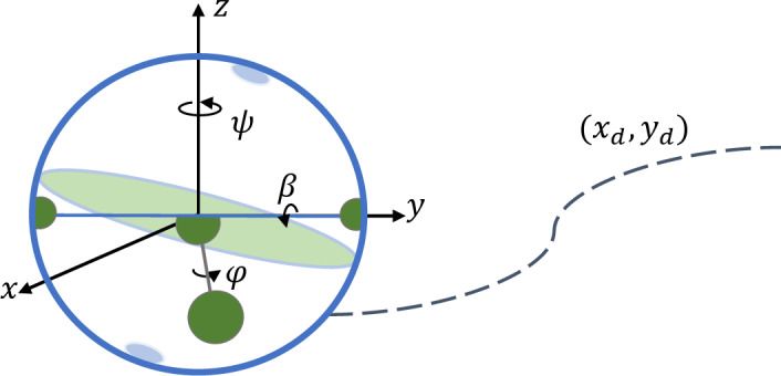
The spherical robot and configuration variables.
System parameters are defined in Table 1.
Table 1.
System parameters.
| Description | Parameter | Description | Parameter |
|---|---|---|---|
| Spherical robot radius |

|
Constraint Matrix |

|
| Robot mass |

|
Jacobian Matrix |

|
Inertia of the spherical robot around the  -axis -axis |

|
Mass matrix |

|
| The x-coordinate of the robot’s center of mass | x | The vector for system kinematic control inputs |

|
Linear velocity of the spherical robot’s center of mass along the  -axis -axis |

|
Derivative of the vector of kinematic control inputs |

|
| The y-coordinate of the robot’s center of mass | y | Coriolis and centripetal forces vector |

|
Linear velocity of the spherical robot’s center of mass along the  -axis -axis |

|
Input torque around the  -axis -axis |

|
Rotation angle of the spherical robot around the  -axis -axis |

|
Input torque around the  -axis -axis |

|
Rotation angle of the spherical robot around the  -axis -axis |

|
Reference trajectory coordinates |

|
Rotation angle of the spherical robot around the  -axis -axis |

|
Obstacle coordinates |

|
Angular velocity of the spherical robot around the  -axis -axis |

|
Distance between the spherical robot and the i-th obstacle |

|
Angular velocity of the spherical robot around the  -axis -axis |

|
Time Horizon |

|
Angular velocity of the spherical robot around the  -axis -axis |

|
Virtual repulsive force |

|
| State vector |

|
Control Parameters of virtual repulsive force functions |

|
| First derivative of state vector |

|
Error vector |

|
| Second derivative of state vector |

|
Derivative of the error vector |

|
| input transformation matrix |

|
MPC cost function |

|
Kinematics model
It is essential to first extract the kinematic and kinetic models of the system. Equation (1) represents the kinematic equations of the spherical robot. These relationships are derived using the rotation matrices obtained from the rotation of the coordinate system attached to the robot, corresponding to the angles  and
and  around a reference coordinate system, as shown in Fig. 1.
 |
1 |
Equation (1) can be expressed as the product of the constraint matrix  and the system generalized velocity vector
  , similar to Eq. 2).
 |
2 |
where
 |
3 |
Therefore, the Jacobian matrix S, which is a full-rank matrix, is derived as follows in order to satisfy the relation  11.
11.
 |
4 |
Assuming  as the system kinematic control inputs vector then the system generalized velocity vector
  can be written as
 |
5 |
Kinetics model
The kinetics model of the system can be derived using the Lagrange method, as outlined below11:
 |
6 |
where  is the system mechanical energy,
  is the input transformation matrix,
  is the torque vector7. Using Eq. (6), system kinetics model can be obtained as
 |
7 |
where  is the vector of Lagrange multipliers and
 |
8 |
 |
9 |
 |
10 |
Multiplying  on Eq. (7) and using
  yields
Equation (12) is the simplified form of Eq. (11).
 |
11 |
Similarly we have
 |
12 |
where
 |
13 |
Alternatively, it can be expressed as
 |
14 |
Finally, the kinetic model of the system can be expressed as
 |
15 |
Model predictive control
In this paper, a predictive control approach is proposed for the control of the kinematics of a spherical robot. Predictive control is a technique that has primarily been utilized in the control of electronic systems, power systems, and chemical plants. This method offers a robust framework for controlling complex systems, particularly those characterized by significant time delays and high-order dynamics. Our application of predictive control aims to guide the spherical robot along a reference trajectory while effectively navigating obstacles with minimal response times.
The key distinction of predictive controllers compared to other control methodologies is their ability to forecast future performance at each step. In contrast, many traditional approaches tend to filter out nonlinear factors, mapping the nonlinear model onto a linear framework.
Kinematic control law
To develop the predictive control law based on the system’s kinematic equations, we will consider the control inputs defined as  and
and  . Consequently, the velocity vector will be expressed as
 |
16 |
In this approach, the system outputs must be initially predicted using a Taylor Series23,24,30. To achieve this, it is essential to first select appropriate candidates to serve as the output functions of the system. In the case of the spherical robot, position errors are selected as the system outputs i.e.
 |
17 |
where
 |
18 |
The objective is for  to converge to zero. The Taylor Series representing the future output errors over the time horizon
  can be expressed as:
 |
19 |
The initial two terms of the expansion have been selected as an approximation for future system errors in order to facilitate predictions of potential inaccuracies. Substituting (18) into (19) yields
 |
20 |
Substituting Eq. (1) into (20) yields
 |
21 |
To evaluate the anticipated performance of the system, we define the cost function J as (24). The function J should incorporate terms that represent the discrepancy between the system’s current position and the desired target. By selecting the cost function as the sum of the squared errors, we ensure that the system’s outputs align closely with the reference outputs.
 |
22 |
Assuming that all tracking errors ( ) hold equal significance, it is established that the weights assigned to all terms in the cost function J are consistent, with the parameters
  and
and  both set at 1/2. Moreover, in the defined function, the control inputs are considered without weights. By minimizing the function J, the appropriate control inputs over the predicted horizon are obtained. The optimality of the cost function
  is conditional upon the vanishing of its partial derivatives with respect to the control inputs as
 |
23 |
which results in
 |
24 |
By substituting Eq. (21) into Eq. (24) and solving the resulting equations, we can derive the control inputs for the spherical robot as
 |
25 |
As prediction horizon  increases, the controller becomes more cautious, emphasizing long-term error minimization and smoother control actions, though excessively large
  may reduce responsiveness. Conversely, a smaller
  prioritizes immediate error reduction, leading to more aggressive control but potentially causing overshoots or instability. The chosen value of
  balances these trade-offs using simulation studies, ensuring prompt responsiveness while maintaining control performance.
Kinetic control law
In this section, we introduce a kinetic control law that utilizes the Lyapunov method. This approach involves establishing an error function for the kinetic system as
 |
26 |
where  is the desired control vector derived from the kinematic control law, and
  .
.
To apply the Lyapunov method, we consider the Lyapunov function candidate, which is defined as a positive definite function as
 |
27 |
The derivative of the Lyapunov function can be expressed as follows
 |
28 |
By substituting  into Eq. (28) yields
 |
29 |
Substituting from Eq. (15) gives
 |
30 |
The kinetic control input can be chosen as
 |
31 |
where the matrix  is the positive definite gain matrix defined as
 |
32 |
By substituting Eq. (32) into (30) results in:
 |
33 |
As can be seen the derivative of the Lyapunov function candidate becomes negative definite for positive definite gain matrices  , leading to the conclusion that the closed loop system for the spherical robot kinetics model is asymptotically stable.
Enhanced predictive control to avoid obstacles
The spherical robot has a variety of applications, including search and rescue operations, inspection tasks, and others. In all these contexts, it is essential for the robot to converge to a predetermined trajectory, which is ideally free from obstacles. Consequently, the control system for the spherical robot must be designed to anticipate and enhance its performance in situations where obstacles are present. The aforementioned control strategy applies to scenarios in which the robot can navigate along the assigned trajectory without any obstacles. However, should an obstacle be encountered, the robot must have the capability to adjust its path temporarily before resuming its original path.
At this stage, the system dynamics should be stabilized around the reference trajectories utilizing the proposed control method. Additionally, this approach has been adjusted using a potential field method to prevent collisions with obstacles. The subsequent equations account for the presence of obstacles, with the distance between the spherical robot and each obstacle being determined as follows:
 |
34 |
where  and
and  are the coordinates of the
  -th obstacle. The virtual repulsive force functions in the
  and
and  directions are defined as14,17:
 |
35 |
In the equations presented above,  represents the adjustable parameter, while
  denotes the diameter or size of the i-th obstacle. The overall resultant repulsive force function, which must be incorporated into the control inputs, is derived as follows:
 |
36 |
If the reference trajectory is identified as  , the deviation error from this reference trajectory, considering the presence of obstacles, is expressed as
 |
37 |
By substituting the error equations derived from Eq. (41) into the control law obtained from solving Eq. (26), the MPC control law in the presence of obstacles is derived as shown in Eq. (42).
 |
38 |
Feedback linearization control
Feedback linearization is a commonly employed technique for controlling nonlinear systems31. This approach enables the transformation of a nonlinear system into a linear framework through the selection of an appropriate input. Following this transformation, a control law can be developed for the system. Recently, there has been considerable research focused on the application of feedback linearization in nonholonomic robots.
Kinematic control law
This section presents the development of a control law for the spherical robot utilizing the existing feedback linearization controller for comparative analysis. The position error of the spherical robot in relation to the desired trajectory, represented by the coordinates  in the Cartesian coordinate system. This is expressed as
  and
and  .
.
It is now presumed that the following asymptotically stable error dynamics apply to the closed-loop kinematic control system.
 |
39 |
Substituting error signals in Eq. (39) results is.
 |
40 |
Substituting  from Eq. (1) into (40) yields the following kinematic control input vector for the system.
 |
41 |
where.
 |
42 |
Stability proof
To prove the stability of control law (42), the Lyapunov function candidate is initially considered as.
 |
43 |
By taking the first derivative of the above relation, we obtain the derivative of the Lyapunov function as.
 |
44 |
By substituting Eq. (1) into (44), we obtain:
 |
45 |
Applying Eq. (41) to Eq. (45) yields.
 |
46 |
Equation (46) illustrates the derivative of the Lyapunov function candidate, which is classified as a negative definite function provided that  and
and  are positive gains. Consequently, this demonstrates that the selected kinematic control is asymptotically stable.
Enhanced feedback linearization control to avoid obstacles
If the spherical robot operated by Feedback Linearization Control (FLC) encounters obstacles, it is essential to enhance the robustness of its control law in response to these obstructions. In this context, the virtual force functions associated with the obstacles, based on Eq. (35), can be used.
As a result, the kinematic control law for the spherical robot, taking into account the presence of obstacles in a manner analogous to Eq. (41) and utilizing error signals derived from Eq. (37), is outlined as follows:
 |
47 |
Stability proof
The positive definite Lyapunov candidate function  is utilized to demonstrate the stability of this control law.
 |
48 |
Thus, the derivative of the Lyapunov function is given by.
 |
49 |
Substituting from Eqs. (1) and (37), results in.
 |
50 |
By substituting from Eq. (47) results in.
 |
51 |
It is important to highlight that, in general, the function xtanh(x) (the product of two odd functions) is always positive. By choosing the coefficients  and
and  as positive gains, we can ensure that the derivative of the Lyapunov function is negative definite within the space
  . This condition guarantees the asymptotic stability of the closed-loop kinematic control system, leading to the convergence of control errors to zero.
Obtained results
In this section, we conduct a comparison and analysis of Model Predictive Control (MPC) and Feedback Linearization Control (FLC) for the motion control of a spherical robot while considering various reference trajectories and the presence of obstacles.
System parameters and corresponding values are given in Table 2.
Table 2.
System parameters and corresponding values.
| Parameter | Value | Parameter | Value |
|---|---|---|---|

|

|

|
2.0 |

|

|

|
1.0 |

|
0.014 
|

|
2.0 |

|
|

|
1.7 |

|

|

|
6.0 |

|


|

|

|

|


|

|

|

|


|

|

|

|

|

|

|

|

|

|


|

|

|

|


|

|
1.0 |

|

|

|
1.0 |

|
0.8 |

|
1.2 |

|
0.5 |

|
1.0 |

|
0.5 |
The block diagram for predictive control and obstacle avoidance of the spherical robot is depicted in Fig. 2.
Fig. 2.

The block diagram for predictive control of the spherical robot.
As illustrated in Fig. 2, the spherical robot tracks the desired trajectory through a control system that integrates both kinematic and dynamic controllers. The kinematic control of the spherical robot is executed utilizing Model Predictive Control (MPC) in one instance and Feedback Linearization Control (FLC) in another. In both scenarios, dynamic control of the spherical robot is governed by a Lyapunov-based approach. Following the implementation of these controllers on the robot’s kinematic system, an analysis and comparison of the robot’s behavior is conducted.
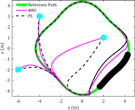
Case-study 1: trajectory tracking in environments containing static obstacles
In this case study, six obstacles are positioned along a diamond-shaped trajectory, and the results are illustrated in Fig. 3. The equations representing the reference trajectory are as follows:
Fig. 3.

Cartesian path for FLC and MPC in tracking diamond-shaped trajectory in an obstacle-rich environment.
 |
52 |
The Cartesian coordinates of the obstacles are outlined as follows:
 |
53 |
It is important to highlight that the control parameters have been carefully chosen to ensure system stability and to deliver ideal performance during each control phase.
Figures 3 and 4 present a comparative analysis of FLC and MPC in terms of their effectiveness in tracking diamond-shaped and spiral trajectories within an obstacle-rich environment.
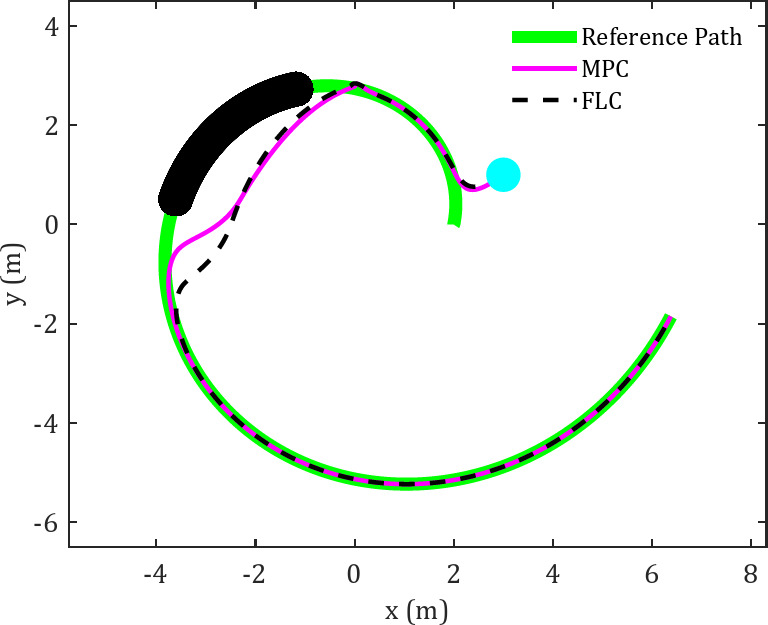
Fig. 4.
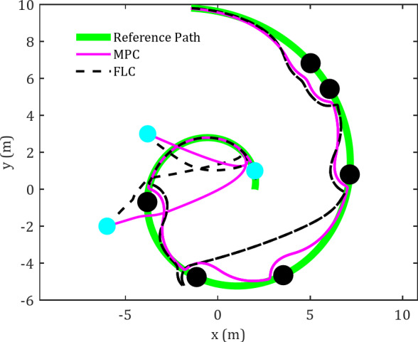
Cartesian path for FLC and MPC in tracking spiral trajectory in an obstacle-rich environment.
The reference trajectories are illustrated in green in the figures. The spherical robot initiates motion from multiple starting positions and progressively aligns itself with the reference trajectory. Preliminary observations suggest that the MPC controller enables the robot to reach the planned trajectory more efficiently. Significantly, when faced with obstacles or unexpected changes in the trajectory, the MPC controller displays enhanced accuracy in converging to the desired trajectory. Under MPC control, the spherical robot shows a more proficient response to obstacles, allowing for closer proximity to them and a reduced time to achieve the desired trajectory compared to the FLC.
Figure 4 illustrates the results of the spherical robot’s motion control using MPC and FLC along a predefined spiral trajectory. This reference trajectory is configured as follows
 |
54 |
The spherical robot starts its motion from three distinct initial points, successfully converging toward the reference trajectory while utilizing two different control methods. An initial evaluation of the trajectory exhibited by the spherical robot under the FLC indicates that the robot converges to the desired trajectory with reasonable accuracy. However, in the presence of obstacles along the trajectory, the performance of the FLC controller deteriorates. In contrast, the MPC controller demonstrates a considerable enhancement in the robot’s capability to follow the reference trajectory. This distinction between the two controllers becomes particularly evident when passing the second and third obstacles. The results further confirm the MPC controller’s superior rate of convergence to the trajectory compared to the FLC controller.
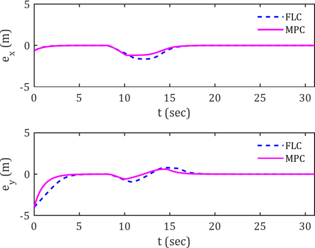
While the path taken by the spherical robot does not enable definitive conclusions regarding temporal variations, the error plots provide validation for these observations. The error plots  and
and  for tracking the diamond-shaped reference trajectory are presented in Fig. 5.
Fig. 5.
Error signals for tracking diamond-shaped reference trajectory along the x and y axes in the presence of obstacles.
Two key points can be discussed here. First, the deviation error is smaller for the MPC controller compared to the FLC controller, indicating that the MPC controller is more resilient to obstacles, allowing the spherical robot to maintain closer proximity to the desired trajectory without excessive deviation when obstacles are present.
Another advantage of the MPC controller over the FLC controller is its faster convergence to the trajectory. This is observed from the shorter distance and time for the error to reach zero in the MPC compared to the FLC. This high trajectory-following accuracy can be attributed to the inherent nature of the MPC controller, which operates based on a forward-looking prediction horizon. In this regard, the appropriate selection of parameter h becomes crucial. For instance, when encountering an obstacle, the MPC controller detects the obstacle’s clearance more quickly than the FLC controller, enabling a faster return to the trajectory. This is because it continuously predicts its trajectory in short, sequential time intervals, optimizing the control inputs.
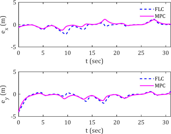
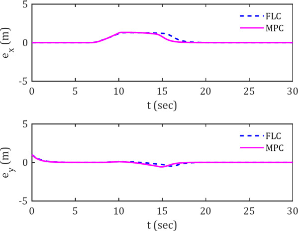
Figure 6 display the deviation error plots for the spiral reference trajectory. Observing the FLC and MPC controller plots, particularly within the 20–30 s time interval, reveals the superiority of the MPC controller in rapidly reducing the error. In other words, the MPC controller tends to keep the spherical robot at a lower deviation from the reference trajectory compared to the FLC controller. This difference between the two controllers becomes more pronounced in the presence of obstacles, as evidenced by the nearly identical behavior of the black and pink curves during the initial 15 s, supporting this assertion.
Fig. 6.

Error signals for tracking spiral reference trajectory along the x and y axes in the presence of obstacles.
Figure 7 illustrates the applied torques in the φ and β channels for the diamond-shaped reference trajectory. This indicates a significant difference in torque variations, as the magnitude of overshoots when encountering obstacles is considerably higher with the FLC controller than with the MPC controller.
Fig. 7.
Actuator torques for tracking diamond-shaped reference trajectory in the presence of obstacles.
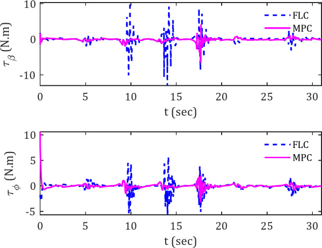
High torque variations are considered an unfavorable characteristic, as they can lead to operational difficulties for the actuators of the spherical robot that are tasked with generating torque. Consequently, while the movement of the spherical robot may seem achievable in proximity to the reference trajectory, implementing this effectively in practice would present significant challenges.
In analyzing Fig. 6, particularly during the first 20 s interval, a noticeable difference in torque values between the MPC and FLC is evident. A comparison of plots 6 and 7 reveals that when the spherical robot, under FLC control, attempts to correct its deviation error, it exerts larger torque values. Conversely, the MPC-controlled spherical robot not only sustains a lower deviation error but also converges to the reference trajectory with smaller torque applications. This observation highlights a potential disadvantage of the FLC controller.
Figure 8 demonstrates the torque variations of the spherical robot when utilizing the two introduced controllers for tracking a spiral trajectory, thereby reaffirming previous assertions.
Fig. 8.

Actuator torques for tracking spiral reference trajectory in the presence of obstacles.
As shown in Tables 3 and 4, the statistical analysis demonstrates that, when comparing Model Predictive Control (MPC) and Feedback Linearization Control (FLC), the error metrics (RMS, MAE, and MSE) are consistently lower for the MPC method. These results are visually represented in the corresponding graphs, where it is evident that MPC achieves a significantly smaller deviation from the reference path. The numerical data further supports this observation, confirming that MPC yields lower error values across all three metrics. This suggests that MPC is more effective in minimizing the error in the system’s performance.
Table 3.
Numerical comparison of FLC and MPC algorithms for error signals and control inputs in tracking diamond-shaped trajectory.
| Averaging criterion |

|

|

|

|

|

|

|

|
|---|---|---|---|---|---|---|---|---|
| RMS | 4.27 | 0.90 | 0.87 | 0.28 | 0.73 | 1.21 | 0.19 | 0.57 |
| MAE | 1.38 | 0.41 | 0.17 | 0.12 | 0.49 | 0.78 | 0.14 | 0.25 |
| MSE | 18.27 | 0.81 | 0.75 | 0.08 | 0.53 | 1.46 | 0.04 | 0.33 |
Table 4.
Numerical comparison of FLC and MPC algorithms for error signals and control inputs in tracking spiral trajectory.
| Averaging criterion |

|

|

|

|

|

|

|

|
|---|---|---|---|---|---|---|---|---|
| RMS | 0.91 | 0.80 | 0.63 | 0.47 | 1.70 | 0.49 | 0.33 | 0.45 |
| MAE | 0.31 | 0.30 | 0.28 | 0.26 | 0.80 | 0.22 | 0.19 | 0.28 |
| MSE | 0.83 | 0.64 | 0.39 | 0.22 | 2.89 | 0.24 | 0.11 | 0.20 |
An important aspect to consider is that, although the control inputs in the FLC method are higher on average compared to MPC, the MPC method achieves lower error values with these relatively smaller control inputs. This observation indicates that MPC is able to produce more accurate results with less control effort, highlighting its efficiency in optimizing the control process.
Case-study 2: trajectory tracking in environments containing moving obstacles
This section aims to assess the precision of the spherical robot’s control system in response to moving obstacles. Figure 9 presents the trajectory tracking diagram associated with following the diamond-shaped trajectory. The moving obstacle, indicated in black on the diagram, attached to the specified trajectory. Regarding the dynamic obstacle avoidance implementation, in the current method, dynamic obstacles and their trajectories are predefined for the control system. This means the predictive control operates under the assumption that information about obstacle positions and trajectories is known in advance. While this approach allows for effective obstacle avoidance in controlled scenarios, it does not currently handle unknown movements or unknown obstacle trajectories in real-time.
Fig. 9.
Cartesian path for FLC and MPC in tracking diamond-shaped trajectory in the presence of moving obstacle.
As can be seen, obtained results indicate that the spherical robot, under MPC control, converges to the reference trajectory with less error compared to the FLC controller after passing the obstacle. At the start of the motion, the difference between the two controllers is noticeably evident. As expected, examining different starting points for the spherical robot reveals that MPC achieves convergence to the trajectory in a shorter time compared to FLC. Another important aspect in analyzing the spherical robot’s motion under the influence of the two controllers is the reduced deviation of the robot when passing near the moving obstacle under MPC control. This means that, when controlled by FLC, the spherical robot maintains a greater lateral distance from obstacles.
In this section, the appropriate selection of the control parameters  and
and  in both controllers is crucial, as these parameters affect the deviation location and the extent of the spherical robot’s deviation from the trajectory.
The above results are also applicable to another candidate trajectory. Figure 10 depicts the trajectory of the spherical robot along the spiral trajectory under the specified controllers. In this diagram, the faster return of the robot after avoiding the obstacle when moving with the MPC controller, compared to the FLC controller, is clearly observed.
Fig. 10.
Cartesian path for FLC and MPC in tracking spiral trajectory in the presence of moving obstacle.
Figure 11 illustrate the tracking error variations of the spherical robot over time in the  and
and  directions along the diamond-shaped trajectory.
Fig. 11.
Error signals in tracking diamond-shaped trajectory along the x and y axes in the presence of moving obstacles.
The results indicate that the deviation error from the trajectory remains in vicinity of zero throughout the trajectory, except for the period when the spherical robot is in proximity to the moving obstacle. The superior resilience of the MPC controller compared to the FLC in handling obstacles can be inferred from the trajectory deviation error graphs. Under MPC control, the spherical robot can maintain an optimal distance to the reference trajectory compared to FLC. The rapid convergence of the graph to zero and the lower trajectory error relative to the desired trajectory under MPC control confirm this claim.
Figure 12 illustrates the trajectory deviation error of the spherical robot while tracking the spiral reference trajectory in the presence of a moving obstacle.
Fig. 12.
Error signals in tracking spiral trajectory along the x and y axes in the presence of moving obstacles.
This further confirm the claim of the MPC controller’s superior performance compared to FLC when encountering moving obstacles. During the time interval of 7–20 s, which includes the interaction with the moving obstacle, the lower error in the MPC graph, as well as its faster convergence to zero compared to the FLC, is evident.
The statistical analysis (Table 5) and graphical results demonstrate that Model Predictive Control (MPC) consistently surpasses Feedback Linearization Control (FLC) in performance, exhibiting lower RMS, MAE, and MSE error values and smaller deviations from the reference trajectory. Notably, MPC achieves superior accuracy with reduced control effort compared to FLC, underscoring its efficiency in optimizing system performance. These findings highlight MPC’s effectiveness in minimizing errors while maintaining lower control inputs.
Table 5.
Numerical comparison of FLC and MPC algorithms for error signals and control inputs in tracking diamond-shaped trajectory in the presence of moving obstacle.
| Averaging criterion |

|

|

|

|

|

|

|

|
|---|---|---|---|---|---|---|---|---|
| RMS | 0.46 | 0.19 | 0.21 | 0.14 | 0.90 | 1.71 | 0.41 | 0.60 |
| MAE | 0.14 | 0.11 | 0.10 | 0.09 | 0.55 | 1.04 | 0.20 | 0.24 |
| MSE | 0.21 | 0.04 | 0.04 | 0.02 | 0.82 | 2.91 | 0.17 | 0.36 |
Conclusion
This paper introduced a predictive control framework tailored for spherical robots, addressing the critical challenges of trajectory tracking and obstacle avoidance in dynamic and static obstacle-dense environments. By utilizing predictive control ability to forecast future states and optimize control inputs, the proposed approach demonstrated superior performance compared to traditional feedback linearization methods. The framework achieved faster response times (on average, less than 10%), reduced control errors (on average, less than 40%), improved settling capabilities (on average, less than 10%), and enhanced adaptability to avoid obstacles. In this study, we conducted a thorough comparison by placing the spherical robot on various trajectories containing both static and dynamic obstacles to evaluate the controllers. Obtained results and case studies highlight the framework’s effectiveness in ensuring precise navigation, robust obstacle avoidance, and overall system stability. This unified approach successfully integrates trajectory tracking with obstacle avoidance, overcoming limitations in existing methods and providing a reliable solution for practical applications. This work advances the state of the art in spherical robot control. It offers an efficient solution for navigating challenging environments, contributing valuable insights to the field of autonomous robotic systems. Future research may focus on expanding the framework with advanced machine learning-based prediction models to further enhance its performance in highly dynamic, uncertain and unpredictable environments. Key areas of exploration include the extension to multi-robot systems, real-world deployment, enhanced dynamic obstacle avoidance, and the examination of three-dimensional environments.
Author contributions
The authors (A. K., P. M. and F. B.) contributed equally to this work.
Data availability
The datasets used and/or analysed during the current study available from the corresponding author on reasonable request.
Declarations
Competing interests
The authors declare no competing interests.
Footnotes
Publisher’s note
Springer Nature remains neutral with regard to jurisdictional claims in published maps and institutional affiliations.
References
- 1.Mercorelli, P. Using fuzzy PD controllers for soft motions in a Car-like robot. Adv. Sci. Technol. Eng. Syst. J.3, 380–390 (2018). [Google Scholar]
- 2.Keymasi Khalaji, A. & Ghane, M. A physically motivated control algorithm for an autonomous underwater vehicle. Proc. Inst. Mech. Eng. Part C J. Mech. Eng. Sci. (2021).
- 3.Dewi, T., Risma, P., Oktarina, Y. & R KusumantoD Motion control analysis of a spherical robot as a surveillance robot. J. Phys. Conf. Ser.1167(1), 012004 (2019). [Google Scholar]
- 4.Zheng, L., Guo, S. & Gu, S. The communication and stability evaluation of amphibious spherical robots. Microsyst. Technol.25 (7), 2625–2636 (2019). [Google Scholar]
- 5.Bicchi, A., Balluchi, A., Prattichizzo, D. & Gorelli, A. Introducing the SPHERICLE: an experimental testbed for research and teaching in nonholonomy. In Proceedings of International Conference on Robotics and Automation. 3, 2620–2625. (1997).
- 6.Joshi, V. A. & Banavar, R. N. Motion Anal. Spherical Mob. Robot Robotica, 27(3), 343–353. (2009). [Google Scholar]
- 7.Halme, A., Schonberg, T. & Yan, W. Motion control of a spherical mobile robot. In Proceedings of 4th IEEE International Workshop on Advanced Motion Control - AMC ‘96 - MIE. 1, 259–264. (1996).
- 8.Sang, S. J., Shen, D., Zhao, J. C., Hu, J. Y. & An, Q. Anal. Simul. Spherical Robot Adv. Mater. Res., 171–172 748–751. (2011). [Google Scholar]
- 9.Bastola, S. & Zargarzadeh, H. Super Twisting Sliding Mode Control of Spherical Robot. In 2019 IEEE International Symposium on Measurement and Control in Robotics (ISMCR). (2019).
- 10.Qiang, Z., Zengbo, L. & Yao, C. A Back-stepping based trajectory tracking controller for a Non-chained nonholonomic spherical robot. Chin. J. Aeronaut.21 (5), 472–480 (2008). [Google Scholar]
- 11.Cai, Y., Zhan, Q. & Xi, X. Path tracking control of a spherical mobile robot. Mech. Mach. Theory. 51, 58–73 (2012). [Google Scholar]
- 12.Taheri Andani, M. et al. Observer-Based Sliding Mode Control for Path Tracking of a Spherical Robot. Complexity. 2018, 3129398. (2018).
- 13.Li, P. et al. UGV navigation in complex environment: an approach integrating security detection and obstacle avoidance control. IEEE Trans. Intell. Veh., 1–14. (2024).
- 14.Keymasi Khalaji, A. & Tourajizadeh, H. Nonlinear Lyapounov based control of an underwater vehicle in presence of uncertainties and Obstacles. Ocean Eng.198, 106998 (2020). [Google Scholar]
- 15.Mehrabani, M. M., Khalaji, A. K. & Ghane, M. Control of a group of uncertain wheeled robots with global inputs in the presence of Obstacles. Proc. Inst. Mech. Eng. Part. K: J. Multi-body Dyn. 237 (1), 177–190 (2023). [Google Scholar]
- 16.Rezvani, N. & Keymasi-Khalaji, A. Adaptive RBFNN-based predictive control for the nanopositioning of an electrostatic MEMS actuator. IET Control Theory Appl.18 (5), 551–565 (2024). [Google Scholar]
- 17.Katona, K., Neamah, H. A. & Korondi, P. Obstacle avoidance and path planning methods for autonomous navigation of mobile robot. Sensors24 (11), 3573 (2024). [DOI] [PMC free article] [PubMed] [Google Scholar]
- 18.Keymasi Khalaji, A. & Moosavian, S. A. A. Switching control of a Tractor-Trailer wheeled robot. Int. J. Robot. Autom., 30(2), (2015).
- 19.Tabatabaee-Nasab, F. S., Moosavian, S. A. A. & Keymasi Khalaji, A. Adaptive fault-tolerant control for an autonomous underwater vehicle. Robotica.40 (11), 4076–4089 (2022). [Google Scholar]
- 20.Keymasi Khalaji, A. & Bahrami, S. Finite-time sliding mode control of underwater vehicles in 3D space. Trans. Inst. Meas. Control. 44 (16), 3215–3228 (2022). [Google Scholar]
- 21.Keymasi Khalaji, A. & Jalalnezhad, M. Stabilization of a tractor with N trailers in the presence of wheel slip effects. Robotica. 39 (5), 787–797 (2021). [Google Scholar]
- 22.Ghasemzadeh, A., Amjadifard, R. & Keymasi-Khalaji, A. Adaptive dynamic programming for trajectory tracking control of a tractor-trailer wheeled mobile robot. IET Control Theory Appl. Article19(1), (2025).
- 23.Mirzaeinejad, H. & Shafei, A. M. Modeling and trajectory tracking control of a two-wheeled mobile robot: Gibbs–Appell and prediction-based approaches. Robotica. 36 (10), 1551–1570 (2018). [Google Scholar]
- 24.Mirzaeinejad, H. Optimization-based nonlinear control laws with increased robustness for trajectory tracking of non-holonomic wheeled mobile robots. Transp. Res. Part. C Emerg. Technol.101, 1–17 (2019). [Google Scholar]
- 25.Nascimento, T. P., Dórea, C. E. T. & Gonçalves, L. M. G. Nonlinear model predictive control for trajectory tracking of nonholonomic mobile robots: A modified approach. Int. J. Adv. Rob. Syst., 15(1), (2018).
- 26.Fareh, R., Khadraoui, S., Abdallah, M. Y., Baziyad, M. & Bettayeb, M. Active disturbance rejection control for robotic systems: A review. Mechatronics. 80, 102671. (2021).
- 27.Azar, A. T. et al. Optimized Model Predictive Control for Unmanned Aerial Vehicles with Sensor Uncertainties. In 2022 International Conference on Control, Automation and Diagnosis (ICCAD), 1–6. (2022).
- 28.Al-Jodah, A. et al. PSO-based optimized neural network PID control approach for a four wheeled omnidirectional mobile robot. Int. Rev. Appl. Sci. Eng.14 (1), 58–67 (2023). [Google Scholar]
- 29.Tutsoy, O., Asadi, D., Ahmadi, K., Nabavi-Chashmi, S. Y. & Iqbal, J. Minimum distance and minimum time optimal path planning with bioinspired machine learning algorithms for faulty unmanned air vehicles. IEEE Trans. Intell. Transp. Syst.25 (8), 9069–9077 (2024). [Google Scholar]
- 30.Mirzaeinejad, H. Robust predictive control of wheel slip in antilock braking systems based on radial basis function neural network. Appl. Soft Comput.70, 318–329 (2018). [Google Scholar]
- 31.Mercorelli, P. Robust feedback linearization using an adaptive PD regulator for a sensorless control of a throttle valve. Mechatronics19 (8), 1334–1345 (2009). [Google Scholar]
Associated Data
This section collects any data citations, data availability statements, or supplementary materials included in this article.
Data Availability Statement
The datasets used and/or analysed during the current study available from the corresponding author on reasonable request.