Adjusting Data to Body Size: A Comparison of Methods as Applied to Quantitative Trait Loci Analysis of Musculoskeletal Phenotypes

Abstract

The aim of this study was to compare three methods of adjusting skeletal data for body size and examine their use in QTL analyses. It was found that dividing skeletal phenotypes by body mass index induced erroneous QTL results. The preferred method of body size adjustment was multiple regression.

Introduction

Many skeletal studies have reported strong correlations between phenotypes for muscle, bone, and body size, and these correlations add to the difficulty in identifying genetic influence on skeletal traits that are not mediated through overall body size. Quantitative trait loci (QTL) identified for skeletal phenotypes often map to the same chromosome regions as QTLs for body size. The actions of a QTL identified as influencing BMD could therefore be mediated through the generalized actions of growth on body size or muscle mass.

Materials and Methods

Three methods of adjusting skeletal phenotypes to body size were performed on morphologic, structural, and compositional measurements of the femur and tibia in 200-day-old C57BL/6J × DBA/2 (BXD) second generation (F₂) mice (n = 400). A common method of removing the size effect has been through the use of ratios. This technique and two alternative techniques using simple and multiple regression were performed on muscle and skeletal data before QTL analyses, and the differences in QTL results were examined.

Results and Conclusions

The use of ratios to remove the size effect was shown to increase the size effect by inducing spurious correlations, thereby leading to inaccurate QTL results. Adjustments for body size using multiple regression eliminated these problems. Multiple regression should be used to remove the variance of co-factors related to skeletal phenotypes to allow for the study of genetic influence independent of correlated phenotypes. However, to better understand the genetic influence, adjusted and unadjusted skeletal QTL results should be compared. Additional insight can be gained by observing the difference in LOD score between the adjusted and nonadjusted phenotypes. Identifying QTLs that exert their effects on skeletal phenotypes through body size-related pathways as well as those having a more direct and independent influence on bone are equally important in deciphering the complex physiologic pathways responsible for the maintenance of bone health.

INTRODUCTION

Many biological phenomena vary with body size, which can confound interpretation when studying differences in measures resulting from factors other than general growth and resultant body size. Variables of interest are often adjusted or “scaled” to a measure of body size specific to the biological function such as leg length for locomotion measures, body weight for lung function, or limb length for muscle mass. Standard measures of body size are body weight, height, and body mass index (BMI = weight divided by length squared).

Ratios are often used to scale both human and animal musculoskeletal data. Muscle mass and strength comparisons are frequently made on body size–adjusted measures. Two methods are typically used to adjust muscle strength: the first is the standard ratio method where muscle strength is divided by body mass, and the second is allometric scaling based on geometric or biological similarity, where muscle strength is divided by body mass or another mass related measure at the power of two-thirds.^(1–3) Comparisons are also made on muscle mass adjusted for height. For example, Zamboni et al.⁽⁴⁾ adjusted appendicular skeletal muscle mass in humans for height by dividing muscle mass by height squared and Masinde et al.⁽⁵⁾ adjusted lean body mass for body length by dividing by body length to identify quantitative trait loci (QTLs) for lean body mass independent of body length in mice. Because many skeletal measures are proportional to size, skeletal measures are often adjusted for both body height and body weight. To obtain a measure of BMD independent of height, Harris and Dawson-Hughs⁽⁶⁾ corrected BMD at the spine and femoral neck by dividing by height, and for total body BMD, they divided by the square root of height. The square root of height was used to adjust total body BMD because total body BMD divided by height was negatively correlated with height (r = −0.26), whereas total body BMD divided by the square root of height was not (r = −0.02). Mechanical properties of bone have also been adjusted to body size. Lochmuller et al.⁽⁷⁾ normalized human cadaver vertebral failure load to body weight, body length, and body weight × body length by dividing by each of these measures separately.

Packard and Boardman⁽⁸⁾ have previously discussed issues associated with using ratios to scale experimental data, and Atchley et al.⁽⁹⁾ used simulated data to show how spurious correlations may arise from using ratios as a method of scaling. For example, if a subsequent analysis is to be performed on measures of gastrocnemius muscle mass (X₁), body size (X₂), and tibial diaphyseal length (X₃) and the intent is to study whether the same genes are influencing muscle mass and bone length independent of overall body size, the investigator may choose to divide bone and muscle measures by body mass index (BMI). The new variables would be muscle mass–scaled (Y = X₁/X₂) and bone-length-scaled (Z = X₃/X₂). When two adjusted variables are derived using a common denominator as in the example above, a spurious correlation can be induced if the CV of the denominator is not equal to the CV of the numerator.⁽⁹⁾ The CV is equal to the SD divided by the mean multiplied by 100.

The CV measures the variability relative to the mean and allows for comparison of the dispersion of different types of data. The ratio of the CV of the variable of interest to the CV of the denominator (scaling variable, i.e., body size) can be used as an indicator of how much spurious correlation is induced relative to the initial correlation of two different variables before scaling with the same denominator. Results from the simulated date of Atchley et al.⁽⁹⁾ showed that as the ratio of the CVs (δ₁/δ₂) decreased from 2 to 0.1, the induced correlation between the new ratio variables Y and Z increased. The initial correlation coefficient between X₁ and X₃ was varied from positive 0.75 to negative 0.75 while holding the correlation of X₁ to X₂ and X₃ to X₂ equal to zero. All cases resulted in an increase in spurious correlation between the adjusted variables Y and Z. As the correlation of X₁ to X₂ and X₃ to X₂ was increased to 0.5 and –0.5 and the ratio of the CVs was decreased from 2 to 0.1, the induced correlation between Y and Z increased. The model of Atchley et al.⁽⁹⁾ nicely showed that using ratios to remove a size effect may actually induce more of a size effect. The larger the CV of the denominator relative to the numerator, the greater will be the induced correlation. Attempting to remove the covariant body size from muscle and bone measures could actually produce an increase in the size effect, an increase in correlation of muscle to bone, and an increase in the correlation of muscle to body size and bone to body size.

The issue of removing size effects is particularly germane to skeletal studies aimed at defining genetic regulation of the skeleton and pathways through which specific genes function. Twin studies⁽¹⁰⁾ as well as inbred mouse studies^(11–13) have confirmed that bone properties are under significant genetic influence. Many factors are known to influence bone mass acquisition, including diet, sex, endocrine factors, mechanical loading, and genetics. Previous studies have also shown that muscle mass is associated with increased bone mass.⁽¹⁴⁾ In addition, body weight and length are significantly correlated with skeletal measures^(15,16) and also have been shown to be under significant genetic influence.^(12,15,16) Distinguishing whether a gene (or chromosomal locus containing a gene) is operating on bone through overall growth and size effects or through actions unrelated to growth is an important first step toward defining the physiologic pathway through which the gene or locus exerts influence.

The mechanical strength of bone is not based solely on density (bone tissue per unit volume) but rather is the result of complex interactions among size, shape, cross-sectional tissue distribution, and mechanical integrity of the matrix itself. By way of example, it has long been known that the cortical expansion of long bones that occurs with age acts partially to offset the effects of age-related bone loss because the redistribution of cortical bone away from the axis of bending increases bending strength, thus a geometric change in bone distribution compensates for a volumetric change in bone mass.

The highest loads normally experienced by bone are from muscle forces used to resist or produce movement. As muscle mass increases the potential load applied to bone increases, with concurrent increases in bone strain. These changes in load presumably modulate the growth, modeling, and remodeling of our skeletons, according to principles commonly referred to as Wolff’s law. A study by Zanchetta et al.⁽¹⁷⁾ of boys and girls between the ages of 2 and 20 showed that bone formation continued as long as muscle mass was increasing and provided a cogent illustration of this concept.

Whereas muscles are thought to provide the largest source of bone strain, body weight is the second biggest intrinsic contributor. The effect of body size, both length and mass, is complex and can interact with physical activity, which also plays a role in the skeletal loading environment. The correlation between body weight and skeletal measures such as cortical thickness or BMD by DXA could also be a result of a simple scaling effect where larger individuals have larger bones, resulting in increased cortical thickness and increased BMD.

QTL analysis is one method that can be used to identify genetic influence of continuously distributed traits. F₂ generation mice are often used in QTL analysis and are produced by first mating two highly inbred progenitor strains such as C57BL/6J (B6) and the DBA/2 (D2) strains, producing an F₁ generation, and then mating the F₁ generation to produce an F₂ generation. The genome of the F₂ generation will vary across each chromosome with three possible allelic states. At each marker, one-quarter of the mice will be homozygous with a B6-B6 allelic state, one-quarter of the mice will be homozygous with a D2-D2 allelic state, and one-half of the mice will be heterozygous with a B6-D2 allelic state. For each individual mouse, the genotype is determined for several markers on each chromosome in the mouse genome, and the genotype of each marker can be in any of the three allelic states because of recombination during meiosis. This variation allows for the isolation of chromosomal intervals that are associated with differences in a phenotypic trait among the individual F₂ mice.

Recently, there have been many studies in the literature reporting QTLs for skeletal measures, such as BMD, bone strength, or cortical thickness, that have co-localized with QTLs for nonskeletal phenotypes such as body weight, body length, and adipose mass.^(18–23) Many of these skeletal measures have been shown to be correlated with body size, suggesting that genetic effects might be mediated through generalized growth and resultant overall body size. Adjusting data to body size allows for the investigation of QTLs that influence skeletal measures independently of body size.

This paper explores statistical issues associated with adjusting skeletal measures to body size in an attempt to remove simple scaling effects. The effects that specific adjustment procedures have on the results of QTL analyses of skeletal data are examined and discussed.

MATERIALS AND METHODS

Animal husbandry

Two hundred male and 200 female F₂ mice derived from C57BL/6J and DBA/2 progenitor strains were examined at 200 days of age. Animal breeding and maintenance were conducted in a specific pathogen-free barrier facility maintained by The Center for Developmental and Health Genetics at The Pennsylvania State University. Mice were weaned into like-sex sibling groups at about 25 days of age with four animals per cage. They were fed a diet of autoclaved Purina Mouse Chow 5010 (content: 1.0% calcium, 0.67% phosphorus, 0.22% magnesium, and 4.4 IU/g vitamin D) ad libitum, designed (after autoclaving) to be equivalent to Purina 5001 (content: 0.95% calcium, 0.67% phosphorus, 0.21% magnesium, and 4.5 IU/g vitamin D). The barrier facility was maintained under positive air pressure with a temperature- and humidity-controlled environment and a 12-h light/dark cycle. All procedures complied with and were approved by the Pennsylvania State University Institutional Animal Care and Use Committee.

Genotyping

All animals were genotyped using 96 microsatellite markers distributed throughout the genome with an average spacing of 15–20 cM. Marker analyses were conducted on purified DNA samples procured from tail snips using an automated, fluorescence-based detection system described in detail in Vandenbergh et al.⁽²⁴⁾

Tissue harvest and gross dimensional measurements

Animal weight was recorded before death by cervical dislocation. Nose-to-anus length was recorded immediately after death. Epididymal fat pads (in males) and uterine fat pads (in females) were dissected and weighed to 0.1 g accuracy on an electronic balance. The right hind limb was harvested, and the gastrocnemius, soleus, tibialis anterior, and extensor digitorum longus muscles were dissected and weighed to the nearest hundredth of a milligram. The femur and tibia were cleaned and stored at −20°C until mechanically tested.

At the time of testing, the bones were thawed at ambient temperature. A digital caliper accurate to 0.01 mm was used to measure femoral length and femoral width at the center of the diaphysis in both the sagittal and coronal planes and epiphyseal width in the coronal plane. Femoral head and neck diameter were also measured. The tibia was measured similarly, except that the proximal, rather than distal, epiphyseal width was measured.

Flexural testing of the right femoral and tibial diaphysis

Femora and tibias were mechanically tested to failure in three-point bending in an MTS MiniBionix 858 testing apparatus (MTS Systems, Eden Prairie, MN, USA) using support spans of 8 (femur) and 10 mm (tibia) and a displacement rate of 1 mm/minute. Femurs were consistently oriented so that the nosepiece was posteriorly directed in respect to the diaphysis. A small section of the anterior flare of the proximal tibia was carefully removed to stabilize the bone on the support span where it was loaded with the anterior cortex in tension. All testing was executed with the bones wet and at ambient temperature. Yield load, yield displacement, energy absorbed at yield, failure load, failure displacement, energy absorbed at failure, and stiffness were determined.

Compositional analysis of the tibia and ash mass of the femur

After mechanically testing the femoral shaft, the femoral bone fragments were ashed in a muffled furnace at 800°C for 24 h to determine femoral ash mass. After flexural testing of the tibia, the distal fragment was dried in a vacuum oven at 100°C for 24 h and ashed at 800°C for 24 h. Percentage water, organic, ash, and mineralization were obtained based on the wet, dry, and ash mass of the tibia.

Tissue processing and histomorphometry

The proximal tibia and previously ashed distal femur were embedded in methyl methacrylate using a three-step three-solution approach.⁽²⁵⁾ A diamond wire saw (Delaware Diamond Knives, Wilmington, DE, USA) was used to cut 150-mm diaphyseal cross-sections. Digital images of each cross-section were collected using a light microscope equipped with a 4× objective and a high-resolution CCD video camera interfaced to a personal computer. Images were captured using NIH IMAGE software (version 1.61; NIH). Total area within the periosteal surface, medullary area within the endosteal surface, cortical area, centroid of the cross-section, cross-sectional moment of inertia (CSMI), average cortical thickness, and distance from the centroid to the tensile periosteal surface were calculated using a MATLAB program (version 6.5, release 13; Math-Works).

Material properties

Cross-sectional data, together with data from the flexural tests, were used to calculate the yield and failure stress (σ = FLc/4I), strain (ɛ = 12cd/L²), and elastic modulus (E = FL³/d48I) of each diaphysis, where σ is the bending stress, F is yield or failure load, L is unsupported span length, c is the distance from the cross-section centroid to the tensile periosteal surface, I is the cross-sectional moment of inertia, and d is the machine displacement. Equations used to calculate material properties were derived from standard beam theory.

Analyses

All phenotypic data were tested for normality, and natural log or square root transformations were used when necessary. The results based on transformed variables are indicated with an (L) for log transformation or an (S) for square root transformation. All analyses were conducted on male and female combined data that were corrected for sex mean differences by subtracting the difference between the male and female mean from each individual male measurement. Variance differences, if present, were retained.

Body size adjustment

Three methods were used to adjust skeletal and muscle phenotypic measurements to body size measures. Initially, skeletal and muscle measures were adjusted to BMI. This adjustment was performed using a ratio method and consisted of dividing each phenotypic measure by BMI. The second method of adjustment was regression of each phenotype against BMI. A third method was also performed, whereby skeletal and muscle phenotypic measures were adjusted using multiple regression against body weight and body length. The regression analyses yielded a residual value for each individual data point, which was subsequently used as the adjusted phenotypic value. All phenotypic data were inspected and contrasted to screen for effects of adjustment. Variables most illustrative of generalized outcomes were selected for further examination of their relative variance. Pearson product moment correlations were also performed on these variables.

QTL analyses

QTL analyses were performed on the F₂ cohort to locate chromosomal regions influencing phenotypic variables using QTL Cartographer software to perform interval mapping.⁽²⁶⁾ QTL analyses were performed on nonadjusted data, data adjusted by dividing with BMI, data adjusted by regressing against BMI, and data adjusted by multiple regression against weight and length. Analyses showing interesting effects of adjustment are presented.

RESULTS

Many skeletal phenotypes were positively correlated with body size and muscle mass phenotypes (Table 1). After adjustment using the BMI ratio method, the correlation of all skeletal phenotypes with BMI and body weight dramatically increased, and the sign of the relationship changed from positive to negative; however, the correlations of skeletal phenotypes with body length decreased and were no longer significant (Table 2). The correlations between skeletal phenotypes and muscle mass also increased substantially after adjustment with the ratio method. The BMI regression method completely removed the correlation of skeletal and muscle phenotypes with BMI and reduced the correlations between musculoskeletal measures and body weight and body length; nevertheless, relationships between those variables remained significant (Table 3). The body size and body length multiple regression method completely removed the correlation of skeletal and muscle phenotypes with BMI, body weight, and body length (Table 4).

Table 1.

Pearson Correlation Coefficients for Nonadjusted Phenotypes

Phenotypes	BMI (kg/m2)	Body weight (g)	Body length (cm)	Gastrocnemius mass (mg)	Tibialis anterior mass (mg)
Body weight (g)	0.85	1
Body length (cm)	0.20	0.68	1
Gastrocnemius mass (mg)	0.29	0.44	0.41	1
Tibialis anterior mass (mg)	0.28	0.41	0.36	0.54	1
Tibia length (mm)	0.21	0.38	0.40	0.42	0.43
Femur length (mm)	0.05	0.25	0.38	0.33	0.36
Femur ultimate load (N)	0.10	0.22	0.26	0.28	0.26
Femur stiffness (L) (N/mm)	0.12	0.21	0.23	0.08	0.16
Femur ash (S) (g)	0.06	0.23	0.35	0.27	0.36
Tibia stiffness (L) (N/mm)	0.16	0.25	0.23	0.15	0.26

Correlations showing significance at the p < 0.01 level are in gray and at the p < 0.05 are bold. Transformed phenotypes are indicated with an (L) for a log or (S) for a square root transformation.

Table 2.

Pearson Correlation Coefficients for Adjusted Phenotypes Using the BMI Ratio Method

Phenotypes	BMI (kg/m2)	Body weight (g)	Body length (cm)	Gastrocnemius mass (mg)	Tibialis anterior (L) mass (mg)
Body weight (g)	0.85	1
Body length (cm)	0.20	0.68	1
Gastrocnemius mass (mg)	−0.45	−0.21	0.24	1
Tibialis anterior mass (L) (mg)	−0.95	−0.75	−0.06	0.58	1
Tibia length (mm)	−0.97	−0.77	−0.10	0.50	0.96
Femur length (mm)	−0.96	−0.75	−0.06	0.53	0.95
Femur ultimate load (N)	−0.56	−0.36	0.10	0.45	0.61
Femur stiffness (L) (N/mm)	−0.90	−0.71	−0.07	0.45	0.89
Femur ash (S) (g)	−0.84	−0.60	0.04	0.52	0.87
Tibia stiffness (L) (N/mm)	−0.85	−0.66	−0.06	0.45	0.86

Correlations showing significance at the p < 0.01 level are in gray and at the p < 0.05 are bold. Transformed phenotypes are indicated with an (L) for a log or (S) for a square root transformation.

Table 3.

Pearson Correlation Coefficients for Adjusted Phenotypes Using the BMI Regression Method

Phenotypes	BMI (kg/m2)	Body weight (g)	Body length (cm)	Gastrocnemius mass (mg)	Tibialis anterior (L) mass (mg)
Body weight (g)	0.85	1
Body length (cm)	0.20	0.68	1
Gastrocnemius mass (mg)	0	0.20	0.36	1
Tibialis anterior mass (L) (mg)	0	0.18	0.32	0.50	1
Tibia length (mm)	0	0.20	0.37	0.38	0.41
Femur length (mm)	0	0.20	0.37	0.32	0.36
Femur ultimate load (L) (N)	0	0.14	0.25	0.26	0.23
Femur stiffness (L) (N/mm)	0	0.11	0.21	0.05	0.14
Femur ash (S) (g)	0	0.19	0.34	0.27	0.36
Tibia stiffness (L) (N/mm)	0	0.11	0.20	0.11	0.22

Correlations showing significance at the p < 0.01 level are in gray and at the p < 0.05 are bold. Transformed phenotypes are indicated with an (L) for a log or (S) for a square root transformation.

Table 4.

Pearson Correlation Coefficients for Adjusted Phenotypes Using the Body Weight and Length Multiple Regression Method

Phenotypes	BMI (kg/m2)	Body weight (g)	Body length (cm)	Gastrocnemius mass (mg)	Tibialis anterior (L) mass (mg)
Body weight (g)	0.85	1
Body length (cm)	0.20	0.68	1
Gastrocnemius mass (mg)	−0.002	0	0	1
Tibialis anterior mass (L) (mg)	−0.004	0	0	0.43	1
Tibia length (mm)	−0.004	0	0	0.27	0.32
Femur length (mm)	−0.003	0	0	0.21	0.27
Femur ultimate load (L) (N)	−0.004	0	0	0.19	0.16
Femur stiffness (L) (N/mm)	0.005	0	0	−0.02	0.08
Femur ash (S) (g)	−0.007	0	0	0.15	0.28
Tibia stiffness (L) (N/mm)	−0.001	0	0	0.04	0.16

Correlations showing significance at the p < 0.01 level are in gray and at the p < 0.05 are bold. Transformed phenotypes are indicated with an (L) for a log or (S) for a square root transformation.

The ratio of the CV of each phenotype (CV_Pheno) over the CV of BMI (CV_BMI) was much <1.0 for most of the traits. This result was because of the relatively large CV of BMI compared with the CV of many of the traits (Table 5).

Table 5.

Descriptive Statistics for Select Variables

Phenotype	Mean	SD	Variance	CV	CVPheno/CVBMI
Body mass index (kg/m2)	2.95	0.33	0.11	11.13	1.00
Body weight (g)	28.19	4.61	21.23	16.35	1.47
Body length (cm)	9.75	0.36	0.13	3.69	0.33
Gastrocnemius (mg)	113.70	16.05	257.57	14.12	1.27
Tibialis anterior (mg)	41.30	4.79	22.93	11.59	1.04
Tibia length (mm)	18.08	0.42	0.18	2.32	0.21
Femur length (mm)	15.81	0.45	0.20	2.84	0.25
Femur ultimate load (N)	18.65	2.70	7.29	14.47	1.30
Femur stiffness (L) (N/mm)	4.64	0.22	0.05	4.74	0.43
Femur ash (S) (g)	0.16	0.01	0.00	6.74	0.61
Tibia stiffness (L) (N/mm)	4.00	0.24	0.06	5.94	0.53

Transformed phenotypes are indicated with an (L) for a log or (S) for a square root transformation.

Interval mapping results for chromosome 13 (Fig. 1) best show the effects of adjustment using the three techniques. BMI, body weight, and body length all mapped to the proximal region of chromosome 13. Only 3 of the musculoskeletal phenotypes mapped to chromosome 13 before body size adjustment, whereas 11 were present after adjustment using the ratio method. After adjustment using the regression methods, the LOD scores of the three musculoskeletal measures noted in the analyses on the nonadjusted data decreased markedly. The additional QTLs indicated using ratio-adjusted data were completely absent. Similar results were seen for the ratio method of adjustment on chromosome 7 with several musculoskeletal traits mapping to chromosome 7 that were not initially present in the unadjusted results (Fig. 2). However, the QTL results for chromosome 7 using the regression adjustment methods produced increased LOD scores for tibialis anterior muscle mass, femur ash mass, and femur ultimate load compared with the unadjusted results.

FIG. 1.

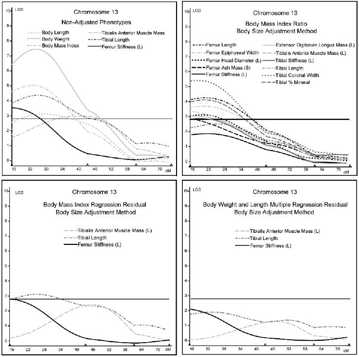
Interval mapping results for chromosome 13. LOD scores are plotted against centimorgan position along the chromosome. The horizontal line indicates the suggestive LOD score threshold of 2.8.

FIG. 2.

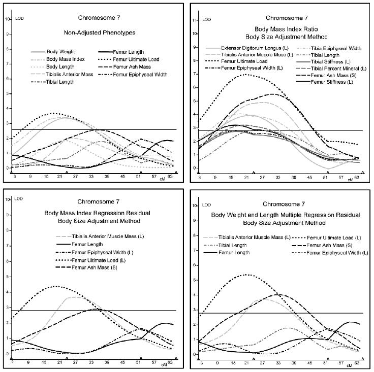
Interval mapping results for chromosome 7. LOD scores are plotted against centimorgan position along the chromosome. The horizontal line indicates the suggestive LOD score threshold of 2.8.

Overall, adjusting musculoskeletal phenotypes for body size through multiple regression yielded very different QTL LOD scores (Table 6). In some cases, LOD scores markedly increased after adjustment with multiple regression, and in other cases, LOD scores decreased.

Table 6.

QTL Results From Interval Mapping

Chromosome 1
Phenotype	Peak cM	LOD Un-Ad	LOD MR	LOD Difference	Increasing Allele
Femur Medullary Area	43.11	3.29	2.56	−0.73	B6
Femur Epiphyseal Width	51.11	2.04	3.18	1.14	D2
Femur Sagital Width	53.11	4.76	4.05	−0.71	B6
Femur Length	72.11	6.20	4.75	−1.45	B6
Tibia Length	74.11	7.96	9.89	1.93	B6
Body Weight	78.11	3.42			D2
Body Length	80.11	3.54			B6
Tibia Total Area	89.21	3.33	3.94	0.62	B6
Tibia CSMI	89.21	3.03	3.83	0.80	B6
Body Mass Index	91.21	3.74			D2
Chromosome 3
Phenotype	Peak cM	LOD Un-Ad	LOD MR	LOD Difference	Increasing Allele
Body Weight	4.41	1.75			B6
Gastrocnemius	6.41	5.11	2.84	−2.27	B6
Body Length	10.41	3.00			B6
Tibia Length	13.81	4.40	2.29	−2.11	B6
Alkaline Phosphatase	13.81	4.20	3.73	−0.46	B6
Chromosome 4
Phenotype	Peak cM	LOD Un-Ad	LOD MR	LOD Difference	Increasing Allele
Body Weight	7.91	2.40			D2
Body Length	27.91	3.58			D2
Tibia Ultimate Load	29.91	3.13	1.90	−1.23	D2
Femur Length	43.91	3.50	1.52	−1.98	D2
Chromosome 6
Phenotype	Peak cM	LOD Un-Ad	LOD MR	LOD Difference	Increasing Allele
Tibia Coronal Width	5.51	2.45	2.94	0.49	B6
Tibia Total Area	5.51	2.57	3.11	0.53	B6
Tibia CSMI	5.51	2.51	3.05	0.54	B6
Tibia Length	7.51	3.09	4.25	1.16	B6
Body Mass Index	11.51	1.69			D2
Tibia Stiffness	13.51	2.87	3.68	0.82	B6
Gastrocnemius	34.51	1.75	3.48	1.74	B6
Tibialis Anterior Mass	40.51	1.95	3.06	1.11	B6
Femur Coronal Width	52.31	5.92	6.74	0.82	B6
Chromosome 7
Phenotype	Peak cM	LOD Un-Ad	LOD MR	LOD Difference	Increasing Allele
Femur Yield Load	17.41	3.54	4.37	0.83	D2
Femur Ultimate Load	19.41	3.61	5.36	1.75	D2
Body Mass Index	21.41	3.36			B6
Body Weight	23.41	3.21			B6
Femur Ultimate Work	24.51	2.49	3.28	0.79	D2
Body Length	24.51	1.76			B6
Tibialis Anterior Mass	26.51	2.01	3.64	1.63	D2
Femur Ash Mass	36.51	2.55	3.95	1.40	D2
Chromosome 11
Phenotype	Peak cM	LOD Un-Ad	LOD MR	LOD Difference	Increasing Allele
Body Length	34.01	3.86			D2
Femur Coronal Width	38.01	3.75	2.47	−1.27	D2
Femur Length	42.01	3.30	2.46	−0.84	D2
Tibia Length	44.01	3.69	2.78	−0.90	D2
Chromosome 13
Phenotype	Peak cM	LOD Un-Ad	LOD MR	LOD Difference	Increasing Allele
Femur Stiffness	16.01	3.54	2.11	−1.43	D2
Body Mass Index	22.01	4.64			D2
Body Weight	24.01	6.61			D2
Tibia Length	26.01	4.37	1.91	−247	D2
Body Length	28.01	3.13			D2
Tibialis Anterior Mass	40.01	2.98	1.40	−1.58	D2
Chromosome 15
Phenotype	Peak cM	LOD Un-Ad	LOD MR	LOD Difference	Increasing Allele
Body Length	35.01	2.49			D2
Femur Yield Load	43.01	2.12	2.98	0.86	B6
Body Weight	43.01	2.14			D2
Femur Ultimate Load	51.91	2.38	3.41	1.03	B6
Chromosome 17
Phenotype	Peak cM	LOD Un-Ad	LOD MR	LOD Difference	Increasing Allele
Body Mass Index	34.01	3.06			B6
Body Weight	42.01	2.20			B6
Femur Yield Load	44.51	2.85	2.42	−0.43	D2
Femur stiffness	54.51	4.68	5.14	0.46	D2

Legend:

Peak cM: Peak centimorgan position for interval.

LOD: Base 10 logarithm of the odds favoring linkage. (Un-Ad-results for unadjusted data, MR-results for multiple regressed residulas)

LOD Difference: Lod score difference between QTL results for unadjusted data and residuals from multiple regression normalization.

Increasing Allele: Genotype of the allele with the increasing additive genetic affect (B6=C575BL/6J, D2=DBA/2)

Shading: QTLs for body size phenotypes (Body mass index, body weight, and body length).

DISCUSSION

Skeletal QTLs often co-localized with QTLs for body weight, body length, and adipose mass. Bone, muscle, and fat are three primary contributors to overall body weight and are highly correlated, making it difficult to determine the operational pathway of these genetic loci. Co-localization could be caused by pleiotropic effects. However, the co-localization of correlated phenotypes to the same locus or chromosomal region is not definitive evidence that there is one gene controlling all of the correlated phenotypes. Because of the substantial number of genes that could be present within the chromosomal region encompassing the QTL, the same region could include several tightly linked genes that influence the correlated phenotypes independently.

Additional insight can be gained by observing the difference in LOD score between the adjusted and nonadjusted phenotypes. A reduction in the LOD score of a skeletal phenotype after adjustment could be indicative of a genetic effect mediated through body size, whereas an increase in LOD score may suggest that a confounding effect was eliminated.

Unadjusted skeletal and muscle phenotypes were strongly correlated with each other, as were skeletal and muscle traits with body size (Table 1). Femur ultimate load and femur ash had correlations of r = 0.26 and r = 0.35 with body length, but after adjusting with the BMI ratio technique (a commonly used scaling method), the correlations with body length were no longer significant. This is likely because of the fact that BMI itself is more strongly correlated with body weight (r = 0.85) than body length (r = 0.20). The correlations between many of the muscle and skeletal phenotypes were consistently higher for ratio-adjusted data compared with the nonadjusted data (Table 2). For example, the correlation of tibial length to tibialis anterior muscle mass increased from r = 0.43 (nonadjusted) to r = 0.96 (ratio adjusted), and the correlation between femur ash mass and BMI, phenotypes that were initially not correlated, increased from r = 0.06 (nonadjusted) to r = 0.84 (ratio adjusted). Attempting to remove the size effect by using the BMI ratio method increased the correlation of each variable with BMI and changed the sign of the relationship.

In general, most morphological measures such as skeletal width and length were more strongly correlated with body length than with body weight, and skeletal strength measures such as tibia ultimate load and muscle mass were more strongly correlated with body weight. However, this was not always the case, and several measures were equally correlated with body length and body weight. Every trait correlated more strongly with either body length or body weight than BMI. BMI has traditionally been used as a way to scale body size, so that the differences between body weight per unit length could be distinguished.

Initially, BMI was used in the regression adjustment method. However, because a stronger correlation is observed between BMI and body weight (r = 0.85) than between BMI and body length (r = 0.2), the residualized data are more correlated with body length than body weight after regression, regardless of whether they were more strongly correlated with length or weight before regression (Table 3). Regression using BMI, by definition, removes all of the variance associated with BMI, but it fails to remove correlations with both body weight and body length. As expected, adjustment by multiple regression completely removes the covariance of body weight and length. After adjustment to body length and body weight using multiple regression, most of the skeletal phenotypes continued to be significantly correlated with muscle phenotypes. However, the correlation was considerably reduced (Table 4). As seen in this work, comparing LOD scores before and after these types of adjustments could be of considerable value when interpreting data from QTL analyses.

The difference in correlation between nonadjusted phenotypes and ratio-adjusted phenotypes clearly indicates an induced correlation increasing the size effect. Using the ratio-adjusted phenotypic data in quantitative trait loci analyses (Figs. 1 and 2) can lead to erroneous results. Analyses for chromosomes 13 and 7 are excellent examples of this effect. Many of the “ratio”-adjusted phenotypes mapped to QTLs associated with body size phenotypes, whereas “non-adjusted” phenotypes did not. For example, tibial coronal width did not map to chromosome 13 initially, but ratio adjustment produced a LOD score >5. On chromosome 13, only three of the traits that mapped on the “ratios” graph were also on the “nonadjusted” graph, and all three of these showed a decrease in LOD score when adjusted using the multiple regression method. The data indicate that multiple regression completely removes size effects, whereas the “ratios” method tends to induce size effects that were not there initially. However, the “ratio” method does not seem to effect the LOD scores for the three traits that mapped to chromosome 13 initially compared with the other traits that mapped to the “ratio” graph in Table 1. The LOD scores for tibial length and femur stiffness did not increase on the “ratios” graph, and the LOD score of tibialis anterior had only a marginal increase, although the peak position shifted to correspond more closely with the LOD score curves for body weight, body length, and BMI. The “ratio” results for tibialis anterior, tibial length, and femur stiffness are somewhat counterintuitive. Going back to our correlation tables, we find that adjusting these phenotypes using the ratio method produced marked increases in their correlation with BMI and a less striking but still significant increase in their correlation with body weight.

The results from chromosome 7 show a similar pattern for the “ratio”-adjusted data, with many traits mapping to the region of the chromosome associated with QTLs for body size phenotypes, trends not seen in the nonadjusted data or data adjusted using the regression technique. Most of the traits that were seen on chromosomes 7 and 13 that mapped to the body size QTL positions had CV ratios (CVRs) <0.5, supporting the argument that these QTLs are the product of correlations induced by the ratio adjustment technique. The multiple regression method of adjustment produced interesting findings for chromosome 7. Tibialis anterior, femur ultimate load, and femur ash mass displayed significant increases in LOD scores after multiple regression adjustment. These three traits were the most affected by multiple regression, and they were also the three traits that scored the highest on the “ratios” graph. This finding could be an indication that the QTL or multiple QTLs on chromosome 7 has or have a direct effect on body size, muscle mass, and skeletal strength, as opposed to acting indirectly through body size, which is likely the case with the QTL on chromosome 13. Alternatively, it could suggest that two closely linked QTLs are present on chromosome 7, with one significantly influencing body size and the other influencing skeletal strength. Removing the variance from skeletal strength that is associated with body size could increase the significance of the skeletal QTL by decreasing the residual “error” variance relative to the true phenotypic value.

In the case of chromosome 13, the multiple regression adjustment method decreased the LOD scores of phenotypes found in the analysis of nonadjusted data. In contrast, the same method produced the opposite effect on the phenotypes associated with loci on chromosome 7, resulting in an increase of LOD scores relative to the nonadjusted data. These inconsistencies could possibly be explained by studying the increase or decrease in LOD score after multiple regression on body weight and length relative to the direction of allelic effect at the locus for body size phenotypes compared with skeletal and muscle phenotypes (Table 6). On chromosomes 3, 4, 11, and 13, the increasing allele for body weight and/or body length is also increasing for muscle and/or skeletal measures, and the result of regressing out body weight and body length was a decrease in LOD score. Conversely, on chromosomes 6, 7, and 15, the increasing allele for body weight and/or body length is opposite to the increasing allele for muscle and/or skeletal measures, and regressing out body weight and body length results in an increase in LOD score. Thus, the decrease in LOD score for femur stiffness, tibia length, and tibialis anterior muscle mass on chromosome 13 after multiple regression is most likely caused by removing the covariance of body weight and length that co-localize to the same region. This is an indication that the genetic influence of this locus on these skeletal measures could be mediated through body size. The increase in LOD scores for the multiple regression phenotypes that co-localized with body weight and length on chromosome 7 is probably caused by removing the covariance of body weight and length that had opposing genetic effects at the same locus. The results for chromosomes 1 and 17 are less clear. On chromosome 1, the D2 allele has an increasing genetic effect for body weight, whereas the increasing allele for body length was B6. For several skeletal phenotypes, regressing out body weight and body length decreased the LOD score, and for a few phenotypes, it increased the LOD score.

In conclusion, as noted, the dangers associated with the use of ratios arrived at by correcting phenotypic data by body weight have been discussed previously,^(8,9) yet this method is still used. The data presented here re-emphasize these dangers. Using this technique in QTL analysis of skeletal traits will almost certainly lead to inaccurate results. Multiple regression is an efficient means of removing variance caused by co-factors to allow for the study of genetic influences independently of correlated phenotypes; however, interpretation of the results is complex. In general, residuals obtained through multiple regression mapped very closely to their unregressed counterparts, but in many cases, the LOD scores were markedly different. Multiple regression should be used to remove the variance of cofactors related to skeletal phenotypes to allow for the study of genetic influence independent of correlated phenotypes. However, the identification of QTLs that exert their effects on skeletal phenotypes through body size–related pathways as well as those having a more direct and independent influence on bone are both important in elucidating genetic influence on bone quality.

The mechanisms involved in bone’s response to its loading environment are complex and involve pathways that are mediated through muscle, activity, and body size. The correlations between body size, muscle mass, physical activity, and skeletal phenotypes can arise through different pathways, and in some cases, produce conflicting responses. Distinguishing between a scaling effect and a response effect is critical in understanding the causal relationships in these complex pathways.

References

- 1.Challis JH. Methodological report: The appropriate scaling of weightlifting performance. J Strength Cond Res. 1999;13:367–371. [Google Scholar]
- 2.Davies MJ, Dalsky GP. Normalizing strength for body size differences in older adults. Med Sci Sports Exerc. 1997;29:713–717. doi: 10.1097/00005768-199705000-00020. [DOI] [PubMed] [Google Scholar]
- 3.Neder JA, Nery LE, Silva AC, Andreoni S, Whipp BJ. Maximal aerobic power and leg muscle mass and strength related to age in non-athletic males and females. Eur J Appl Physiol Occup Physiol. 1999;79:522–530. doi: 10.1007/s004210050547. [DOI] [PubMed] [Google Scholar]
- 4.Zamboni M, Zoico E, Scartezzini T, Mazzali G, Tosoni P, Zivelonghi A, Gallagher D, De Pergola G, Di Francesco V, Bosello O. Body composition changes in stable-weight elderly subjects: The effect of sex. Aging Clin Exp Res. 2003;15:321–327. doi: 10.1007/BF03324517. [DOI] [PubMed] [Google Scholar]
- 5.Masinde GL, Li X, Gu W, Davidson H, Hamilton-Ulland M, Wergedal J, Mohan S, Baylink DJ. Quantitative trait loci (QTL) for lean body mass and body length in MRL/MPJ and SJL/J F(2) mice. Funct Integr Genomics. 2002;2:98–104. doi: 10.1007/s10142-002-0053-7. [DOI] [PubMed] [Google Scholar]
- 6.Harris SS, Dawson-Hughes B. Weight, body composition, and bone density in postmenopausal women. Calcif Tissue Int. 1996;59:428–432. doi: 10.1007/BF00369205. [DOI] [PubMed] [Google Scholar]
- 7.Lochmuller EM, Eckstein F, Kaiser D, Zeller JB, Landgraf J, Putz R, Steldinger R. Prediction of vertebral failure loads from spinal and femoral dual-energy X-ray absorptiometry, and calcaneal ultrasound: An in situ analysis with intact soft tissues. Bone. 1998;23:417–424. doi: 10.1016/s8756-3282(98)00127-6. [DOI] [PubMed] [Google Scholar]
- 8.Packard GC, Boardman TJ 1987 The misuse of ratios to scale physiological data that vary allometrically with body size. In: New Directions in Ecological Physiology. Cambridge University Press, Cambridge, UK, pp. 216–239.
- 9.Atchley WR, Gaskins CT, Anderson D. Statistical Properties of Ratios. I. Empirical Results. Syst Zool. 1976;25:137–148. [Google Scholar]
- 10.Dequeker J, Nijs J, Verstraeten A, Geusens P, Gevers G. Genetic determinants of bone mineral content at the spine and radius: A twin study. Bone. 1987;8:207–209. doi: 10.1016/8756-3282(87)90166-9. [DOI] [PubMed] [Google Scholar]
- 11.Beamer WG, Donahue LR, Rosen CJ, Baylink DJ. Genetic variability in adult bone density among inbred strains of mice. Bone. 1996;18:397–403. doi: 10.1016/8756-3282(96)00047-6. [DOI] [PubMed] [Google Scholar]
- 12.Klein RF, Mitchell SR, Phillips TJ, Belknap JK, Orwoll ES. Quantitative trait loci affecting peak bone mineral density in mice. J Bone Miner Res. 1998;13:1648–1656. doi: 10.1359/jbmr.1998.13.11.1648. [DOI] [PubMed] [Google Scholar]
- 13.Shimizu M, Higuchi K, Kasai S, Tsuboyama T, Matsushita M, Mori M, Shimizu Y, Nakamura T, Hosokawa M. Chromosome 13 locus, Pbd2, regulates bone density in mice. J Bone Miner Res. 2001;16:1972–1982. doi: 10.1359/jbmr.2001.16.11.1972. [DOI] [PubMed] [Google Scholar]
- 14.Kaye M, Kusy RP. Genetic lineage, bone mass, and physical activity in mice. Bone. 1995;17:131–135. doi: 10.1016/s8756-3282(00)00164-2. [DOI] [PubMed] [Google Scholar]
- 15.Keightley PD, Hardge T, May L, Bulfield G. A genetic map of quantitative trait loci for body weight in the mouse. Genetics. 1996;142:227–235. doi: 10.1093/genetics/142.1.227. [DOI] [PMC free article] [PubMed] [Google Scholar]
- 16.Ishikawa A, Matsuda Y, Namikawa T. Detection of quantitative trait loci for body weight at 10 weeks from Philippine wild mice. Mamm Genome. 2000;11:824–830. doi: 10.1007/s003350010145. [DOI] [PubMed] [Google Scholar]
- 17.Zanchetta JR, Plotkin H, Alvarez Filgueira ML. Bone mass in children: Normative values for the 2–20-year-old population. Bone. 1995;16:393S–399S. doi: 10.1016/8756-3282(95)00082-o. [DOI] [PubMed] [Google Scholar]
- 18.Lang DH, Sharkey NA, Mack HA, Vogler GP, Vandenbergh DJ, Blizard DA, Stout JT, McClearn GE. Quantitative trait loci analysis of structural and material skeletal phenotypes in C57BL/6J and DBA/2 second generation and recombinant inbred mice. J Bone Miner Res. 2005;20:88–99. doi: 10.1359/JBMR.041001. [DOI] [PMC free article] [PubMed] [Google Scholar]
- 19.Li X, Masoned G, Gu W, Wergedal J, Mohan S, Baylink DJ. Genetic dissection of femur breaking strength in a large population (MRL/MpJ X SJL/J) of F2 mice: Single QTL effects, epistasis, and pleiotropy. Genomics. 2002;79:734–740. doi: 10.1006/geno.2002.6760. [DOI] [PubMed] [Google Scholar]
- 20.Klein RF, Turner RJ, Skinner LD, Vartanian KA, Serang M, Carlos AS, Shea M, Belknap JK, Orwoll ES. Mapping quantitative trait loci that influence femoral cross-sectional area in mice. J Bone Miner Res. 2002;17:1752–1760. doi: 10.1359/jbmr.2002.17.10.1752. [DOI] [PubMed] [Google Scholar]
- 21.Drake TA, Schadt E, Hannani K, Kabo JM, Krass K, Colinayo V, Greaser LE, III, Goldin J, Lusis AJ. Genetic loci determining bone density in mice with diet-induced atherosclerosis. Physiol Genome. 2001;5:205–215. doi: 10.1152/physiolgenomics.2001.5.4.205. [DOI] [PubMed] [Google Scholar]
- 22.Beamer WG, Shultz KL, Churchill GA, Frankel WN, Baylink DJ, Rosen CJ, Donahue LR. Quantitative trait loci for bone density in C57BL/6J and CAST/EiJ inbred mice. Mamm Genome. 1999;10:1043–1049. doi: 10.1007/s003359901159. [DOI] [PubMed] [Google Scholar]
- 23.Masinde GL, Li X, Gu W, Wergedal J, Mohan S, Baylink DJ. Quantitative trait Loci for bone density in mice: The genes determining total skeletal density and femur density show little overlap in F2 mice. Calcif Tissue Int. 2002;71:421–428. doi: 10.1007/s00223-001-1113-z. [DOI] [PubMed] [Google Scholar]
- 24.Vandenbergh DJ, Heron K, Peterson R, Shpargel KB, Woodroofe A, Blizard DA, McClearn GE, Vogler GP. Simple Tests to Detect Errors in High-Throughput Genotype Data in the Molecular Laboratory. J Biomol Tech. 2003;14:9–16. [PMC free article] [PubMed] [Google Scholar]
- 25.Recker R 1983 Bone Histomorphometry: Techniques and Interpretation. Franklin Book Company, Elkins Park, PA, USA.
- 26.Wang S, Basten CJ, Zeng ZB 2001–2004 Windows QTL Cartographer 2.0. Department of Statistics, North Carolina State University, Raleigh, NC, USA.