

Abstract
In slope stability analysis, identifying the critical slip surface has always been a complex challenge. This study proposes a method to determine the critical slip surface of heterogeneous slopes while accounting for anisotropy. This method is grounded in a generalized soil anisotropic constitutive model and establishes a global equilibrium framework. It integrates global optimization techniques and employs the well-established Morgenstern-Price method to formulate the optimization objective function. The reliability, applicability, and stability of the method are demonstrated through comparative analysis with the results of two classical slope cases and the improved log-spiral limit equilibrium method. Additionally, the study investigates the impact of anisotropy-related parameters on the stability of heterogeneous slopes, providing new insights into how anisotropy influences slope stability and failure mechanisms.
Keywords: Slope stability, Anisotropy, Safety factor, Critical slip surface
Subject terms: Engineering, Civil engineering
Introduction
Stability analysis of both natural and artificial slopes is a prominent issue in civil, geotechnical, and mining engineering. However, the presence of multi-scale discontinuities such as bedding planes, joints, fissures, and faults in natural rock masses introduces significant directional dependence in their mechanical properties1,2. This anisotropy poses new challenges for slope stability analysis. Therefore, understanding how to search for anisotropic slip surfaces and accurately quantify the safety factor is essential for better grasping slope failure mechanisms3,4.
Anisotropy in geotechnical materials is widespread in slope engineering. Different from homogeneous slopes, the stability of anisotropic slopes is influenced by the direction and degree of anisotropy in the strata. Current research methods addressing this issue include field monitoring5–7, kinematic analysis8, limit equilibrium methods9,10, limit analysis, and numerical computations11. In recent decades, researchers such as Kumar6 and Tan5 have conducted extensive field studies on the failure mechanisms of anisotropic slopes. These monitoring results have enhanced our understanding of anisotropy in practical engineering contexts. However, in-situ monitoring facilities may be limited in their ability to capture the entire failure evolution process of anisotropic slopes.
Consequently, numerical methods based on the finite element method, finite difference method, and material point method have been developed. Within these methods, the calculation strategies for anisotropic slope stability analysis can be categorized into three types: (I) constitutive models for anisotropy, (II) spatial variability of strata, and (III) pre-existing layered joints. These approaches address anisotropy at different scales. In the first category, researchers such as He et al.12, Badakhshan et al.13, and Nagendran et al.14 have applied various constitutive models to study anisotropic slope stability, advancing and refining stability analysis. In contrast, Griffiths and Fenton15 and Wang et al.16 adopted probabilistic finite element methods in investigating the failure characteristics and probabilities of transversely anisotropic slopes. Chen17 employed stochastic finite difference methods in probabilistic assessments to quantitatively evaluate the impact of general anisotropic spatial variability on slope reliability. Additionally, with advancements in numerical algorithms, techniques such as contact algorithms, discontinuous methods, and advanced meshing have been proposed to address the distribution of layered joints within rock slopes. Utilizing these algorithms, Tan et al.5 and Zang et al.18 have investigated the stability evolution of slopes with different joint distributions.
When dealing with non-circular failure surfaces, the number of control variables exceeds three, rendering the geometric grid method impractical. Due to its accuracy and straightforward application, the limit equilibrium method (LEM) has become a widely used technique in slope stability analysis. This method generally involves two main tasks: calculating the safety factor and identifying the critical slip surface. For simple slope structures, the slip surface is often assumed to be circular, with calculations performed using the Fellenius method19 or the simplified Bishop method20. The LEM is frequently combined with global optimization algorithms to identify the critical slip surface21. With advancements in computer hardware and optimization algorithms, research on the limit equilibrium method has progressed rapidly. Identifying the critical slip surface involves complex multi-constraint, multi-parameter optimization problems. Researchers have employed evolutionary algorithms22, quasi-physical intelligent algorithms23, population-based optimization algorithms24, and hybrid intelligent algorithms25 to find optimal objective function values, effectively addressing this complex issue. In studies on slope stability calculations using optimization algorithms, factors such as seismic activity26, seepage27, and external loads28 have been considered.
Existing research on slope stability has mainly focused on the anisotropy and spatial variability of geotechnical materials. Chen17 used the limit analysis upper bound method to derive stability solutions for slopes composed of anisotropic, heterogeneous clay. Stockton3 refined the traditional logarithmic spiral limit equilibrium method, extending it to stability analysis of soils with anisotropic cohesion and friction, and studied the impact of shear strength anisotropy on the depth of tensile cracks in slope engineering. Considering soil heterogeneity, researchers such as Karni and Shamrani29 and Dong et al.30 have used the limit equilibrium slice method to study the impact of strength anisotropy on slope stability. A finite element limit analysis method has enabled a more precise evaluation of the ultimate bearing capacity31. Building on this approach, Lai32 integrated an anisotropic undrained failure criterion to examine the undrained stability of tunnel portals with rigid walls in anisotropic clays. In parallel, Izadi33,34 and Pishvari et al.35 assessed the bearing capacity of foundations under cross-anisotropic and complex loading conditions using the second-order cone programming method. Additionally, numerous scholars have applied the random field theory proposed by Vanmarcke36 to slope stability analysis. Gravanis et al.37 integrated random field theory with the LEM to account for spatial variability in the parameters of soil strength. Huang et al.38, Liu et al.39, and Li et al.40 used the autocorrelation function combined with the Cholesky decomposition method to simulate random fields to investigate the impact of rotational anisotropy on slope failure mechanisms and stability. In slope stability analysis methods that combine global optimization techniques with limit equilibrium theory, the consideration of anisotropy remains insufficient. Therefore, it is necessary to establish a method for locating the critical slip surface that can be applied to heterogeneous and anisotropic geological environments.
In this study, we extend a generalized anisotropic constitutive model into the limit equilibrium framework, building upon previous research utilizing the limit equilibrium method. We first establish global equilibrium equations at the element scale that account for anisotropy. These equations are then extended to the soil strip scale and integrated with the objective function from the Morgenstern-Price method. By employing global optimization techniques, the position of the critical slip surface can be accurately located. Overall, the innovative features of our developed method can be summarized as follows,
Through comparisons with multiple case studies, our results demonstrate excellent applicability across geological conditions of varying complexity.
By integrating an improved constitutive model into a generalized slip surface search framework, the approach ensures scalability for diverse geotechnical scenarios.
The method resolves the longstanding limitation of conventional slip surface search techniques in addressing anisotropic strata, which achieving capture of the anisotropic strength characteristics.
The paper is structured as follows. Our new slope stability analysis method considering material anisotropy is derived and introduced in Section “Method for searching critical sliding surface”. In Section “Numerical validation”, we analyze three classical cases to demonstrate the numerical implementation process and conduct a robustness analysis of the proposed method. Section “Numerical results and discussions” presents numerical experimental results, systematically examining the effects of slope angle and anisotropy ratio on slope stability. Finally, we draw conclusions in Section “Conclusions”.
Method for searching critical sliding surface
This chapter introduces a method for analyzing slope stability that takes into account the anisotropy of geotechnical materials. Section “Global equilibrium equations for anisotropic slopes” presents the global equilibrium equations for analyzing anisotropic slopes. Section “Generation of trial sliding surfaces” covers the model for generating trial slip surfaces. Section “Mechanical analysis for safety factor” details the methods for calculating the safety factor. Finally, Section “Optimization algorithm for slop stability analysis” introduces the firefly optimization algorithm used in the search for slip surfaces.
Global equilibrium equations for anisotropic slopes
The LEM analyzes the slope stability by applying the mechanical equilibrium conditions of the sliding body. As depicted in (Fig. 1), we define the landslide body  as the region bounded by both the slope surface
  and the sliding surface
  with a dip angle
  . Normally, the landslide body is primarily influenced by gravitational, seismic, and external forces along the slope. When the sliding body is in the critical state, the following conditions for both force equilibrium and the critical limit equilibrium should be satisfied.
 |
1a |
 |
1b |
 |
1c |
where  and
and  represent the direction vectors in the horizontal and vertical components of stress at a point on the sliding surface, respectively. The parameter
  represents the vertical distance between the slope surface and the sliding surface at a certain point;
  denotes the density,
  is the gravitational acceleration,
  and
and  are the normal and tangential stress, respectively, can be expressed in the form as:
 |
2a |
 |
2b |
where  ,
,  and
and  are the stress components acting upon an infinitesimally small rock mass element, as shown in (Fig. 1).
Fig. 1.
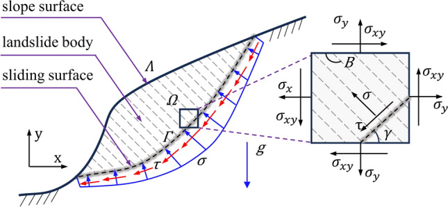
Schematic of the potential sliding surface search and stress analysis.
The evolution of the internal structure is deeply associated with the macroscopic mechanical behavior of granular materials. According to the hypothesis proposed by Booker and Davis41, the mean normal stress  and the principal stress direction
  are available for the characterization of the anisotropic yield surfaces of granular materials. Building on this hypothesis and consistent with experimental evidence that the internal friction angle is relevant to the direction of principal stress, Yuan et al.42 considered the yield surface in the stress space of deviatoric stress as an ellipse (Fig. 2), the anisotropic yield criterion can be written as follows:
 |
3a |
 |
3b |
where  can be defined as the yield function, and
  represents the distance from the stress point to the origin of the coordinate system.
  is defined as the Anisotropic Increase Factor (AIF), and it plays a crucial role in capturing the anisotropic characteristics of strength.
  is the thermodynamic force associated with mean normal stress
  . The parameters
  and
and  are the cohesion and the internal friction angle, respectively, where,
  is the maximum peak internal friction angle and
  is the minimum peak internal friction angle.
Fig. 2.

The yield criterion considering the anisotropy: (a) yield surface in the principal stress space of three dimension and (b) yield surface in stress space of deviatoric stress.
For the point on the sliding surface, the AIF varies with the principal stress direction due to the consideration of the elliptic geometry, and is defined by the following formula:
 |
4 |
Here,  is the angle of the bedding plane measured counterclockwise from horizontal. It corresponds to the direction angle of the
  and ranges from
  to
to  ;
;  is defined as the anisotropy ratio, which is used to represent the ratio of
  to
to  , and is used to represent the anisotropy ratio. The value of
  ranges between 0 and 1. A smaller value of
  indicates a greater degree of anisotropy which was expressed by
  , and when
  , it recovers the isotropic Mohr–Coulomb yield criterion.
As indicated in Fig. 2, the cross-section of the anisotropic yield criterion is assumed to take the form of a rotated ellipse. With  as a center point, the rotation angle of the ellipse is associated with the bedding plane angle, and the length of the major and minor axes of the ellipse is determined by
  and
and  .
.
 |
5 |
Combining Eqs. (1) ~ (5), we can obtain that:
 |
6 |
Equation (6) is the limiting equilibrium condition modified by the anisotropic yield criterion.
The factor of safety  can be used as a crucial design criterion in slope stability analysis. With the aim of preventing potential failures, the slope stability analysis efforts are dedicated in determining the factor of safety
  . According to stability criterion, safety factor is given by:
 |
7 |
where  is the shear resistance acting on a point of the sliding surface, and
  is the components of the forces acting on a point of the sliding surface that cause instability, which can be expressed as:
 |
8a |
 |
8b |
In this study, the LEM is used to identify the critical sliding surface and calculate the value of  corresponding to this critical sliding surface. Therefore, the problem of searching the sliding surface can be defined as an optimization problem.
 |
9 |
Generation of trial sliding surfaces
In order to locate the position of the critical sliding surface, a method proposed by Cheng43 for the generation of non-circular trial sliding surface is adopted. Establish a Cartesian coordinate system with the origin at  , as illustrated in (Fig. 3).
Fig. 3.
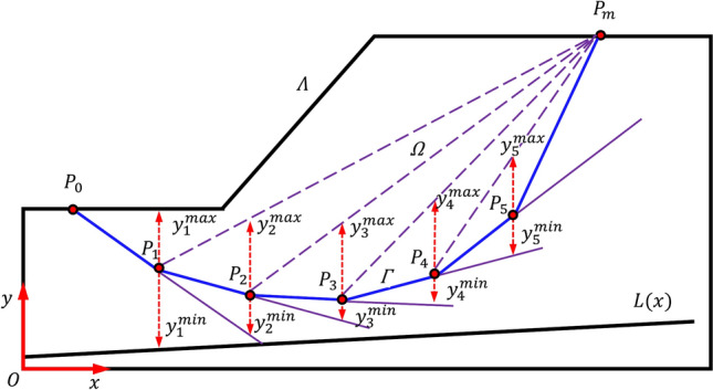
Generation of a non-circular sliding surface.
The method of slices involves dividing the failed soil mass into  vertical slices. Within the framework of Chen’s method, the generated critical slip surface is essentially formed by creating soil slices and combining the bases of these slices to form the slip surface. Therefore, the sliding surface will be described using multiple control points
  ,
,  , …,
, …,  , i.e.
 |
10 |
The width of all slices is set to a fixed value, and the x-coordinate of all control points can be easily determined according to the position of  and
and  , as
, as
 |
11 |
To ensure the geometric topological requirement of being concave upward, the dynamic bound proposed by Cheng43 is used to limit the position of each control point. Based on the known y-coordinates of  and
and  , the y-coordinates of points
  through
  are determined by the slope geometry and the alignment of the known points, sequentially.
For each point except the two endpoints, define the upper bounds as  and the lower bounds as
  . A detailed procedure for determining the upper and lower bounds can be referenced in Cheng’s study43, and their values are defined according to the following formula:
 |
12a |
 |
12b |
where  represent the bed rock surface.
Finally, to ensure the geometric topology of each sliding surface,  is used to map the y-coordinate value, which means the imaginary variable corresponding to variable
  and
and  . In this case,
  is determined by the following formula:
 |
13 |
Mechanical analysis for safety factor
The Morgenstern-Price method is suitable to calculate the factor of safety of sliding surfaces with arbitrary shapes. In this study, we calculate  according to the assumption of the Morgenstern-Price method, as follows:
 |
14 |
where,  represents the normal force of the interslice and
  is the interslice shear force;
  is the direction of action of the interslice force;
  is the scaling factor, which can be obtained from the moment equilibrium of slice
  ; and
; and  is a continuous function of the inter-slice force, and
  .
.  is the ratio between the vertical and lateral interslice forces. Figure 4 illustrates the mechanical model of the Morgenstern-Price method for calculating the slope safety factor. As shown in Fig. 4, the sliding body is discretized into a certain number of vertical slices, each slice has the same safety factor, and a certain soil slice was taken as an isolation for analysis as (Fig. 4).
Fig. 4.
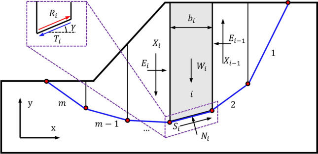
Diagram of Morgenstern-Price method for critical slip surface.
According to Zhu44, the half-sine function is adopted as the interslice function:
 |
15 |
in which  and
and  are the specified non-negative values, and
  ,
,  .
.
In the limit equilibrium analysis using Morgenstern-Price method, the stress pair  of any point on the potential sliding surface is assumed to be lie on the Mohr–Coulomb failure envelope with the reduced strength parameters, as expressed:
 |
16a |
 |
16b |
where  and
and  are the reduced strength parameters.
In this study, to account for the effect of anisotropy in slope stability analysis, we use the anisotropic Mohr–Coulomb failure criterion proposed in Section “Global equilibrium equations for anisotropic slopes” as the limit equilibrium condition. In this framework, the relationship between  and the principal stress direction
  is employed to capture the directional variation of the strength parameters. Based on the assumptions about the interslice forces and considering the force equilibrium of the slice
  , it can be obtained that:
 |
17a |
 |
17b |
For slice  ,
,  is the normal force;
  is the mobilized shear strength;
  is the weight;
  is the width;
  is the dip angle;
  and
and  ,
,
According to Eq. (17 are the shear interslice forces acting on the left and right boundaries of the slice, respectively.), we can obtain:
 |
18 |
where  is the sum of the shear resistances acting lie on the slide line; and
  is the sum of the forces that tending to cause instability. The resultant force
  and
and  are expressed as:
 |
19a |
 |
19b |
By introducing the following variables
 |
20a |
 |
20b |
Equations (17) to (20) incorporate the anisotropic strength characteristics into the limit equilibrium analysis through the introduction of the AIF  . Consequently, we obtain the simplified form of Eq. (18) as:
 |
21 |
Hence, the implicit expression of the factor of safety is derived as follows:
 |
22 |
In the calculation process of the Morgenstern-Price method,  is computed iteratively. To this end, initial values for
  and
and  need to be assumed. To ensure effective transmission of pressure, the initial values of
  and
and  are restricted as:
 |
23a |
 |
23b |
According to the moment equilibrium of the side surface,  can be obtained by the following equation:
 |
24 |
By iterating the above process, the difference between the values of  and
and  calculated in each iteration can be reduced to within the acceptable tolerance
  and
and  . Figure 5 presents the flowchart for calculating
  considering the anisotropic yield criterion.
Fig. 5.

Computational flowchart of Morgenstern-Price method.
Optimization algorithm for slop stability analysis
To enhance the efficiency and accuracy of searching for the critical sliding surface of slopes, researchers have explored various global optimization algorithms45. In the approach to analysis the slope stability considering anisotropy presented in this paper, the global optimization algorithm (Firefly Algorithm) in the artificial intelligence method is used for localization of critical sliding surfaces of slopes. In this study, the firefly algorithm is adopted based on the following two considerations46: (1) the algorithm’s ability to simultaneously search for both global and local optimal solutions; and (2) the characteristic of low interaction among subregions, which significantly improves computational efficiency. Two key aspects of the firefly algorithm (FA) are the calculation of light intensity and the formulation of attractiveness47. The brightness of each firefly is determined by its safety factor; the lower the safety factor, the higher the brightness, which in turn directs the individual to move toward other fireflies. A higher brightness value usually indicates a better solution, but this depends on the specific optimization problem and how the fitness function is defined. In this study,  is used to represent the current position of fireflies
  . For a population size of
  fireflies, the brightness
  of the firefly
  can be defined as follows:
 |
25 |
where  is the function for safety factor computation and the sliding surface function
  can be rewritten to the form in Eq. (26) according to the imaginary variable definition mentioned in Section “Generation of trial sliding surfaces”.
 |
26 |
In the framework of FA, the fireflies with lower brightness values will move towards the fireflies with higher brightness values according to the present movement criteria. We can define the function of the attractiveness as follows:
 |
27 |
where  is Euclidean distance between any two fireflies and
  denotes the attractiveness for
  .
.  is the light absorption coefficient, usually taken as a constant. In addition, regarding a problem in
  dimensions, the Euclidean distance between fireflies
  and
and  can be defined as the following formula:
 |
28 |
in which  represents the parameter value of the
  -th dimension for firefly
  .
.
Then, according to the movement rule defined by FA, the dimmer firefly is drawn towards the brighter one. The movement is determined by Eq. (29).
 |
29 |
It should be noted that  is the randomization parameter between -0.5 and 0.5, introduces variability into the firefly movement. The appropriate step size will directly affect both the global and local search ability of the algorithm. So, set a value for the attenuation factor
  and initial value of the randomization parameter
  , the dynamic parameter
  can be defined by Eq. (30).
 |
30 |
In general, Eqs. (25) and (26) define the objective function, while Eqs. (27) to (30) outline the calculations for the necessary parameters and the movement criteria of the fireflies during the execution of the algorithm. To clearly state the numerical implementation of FA for locating critical slip surface, the algorithmic overview is presented in (Algorithm 1).
Algorithm 1.
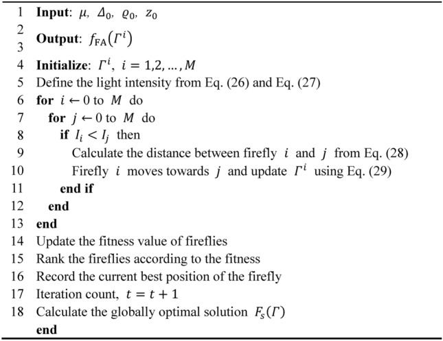
Numerical implementation of FA for locating critical slip surface.
Numerical validation
This section presents numerical results obtained using the proposed analysis method. To verify the applicability and robustness of the proposed method, we report two typical benchmarks of isotropic slope and one anisotropic slope. Section “Slope in single soil layer” begins with a simple homogeneous slope to validate the reliability of the method in single soil layer condition. Section “Slope with weak interlayer” then analyzes a heterogeneous slope with a weak interlayer to verify the applicability of the proposed method under complex soil layer conditions. Subsequently, Section “Anisotropic slope with bedding plane” uses the proposed method to analyze slopes with different bedding plane angle, which further validating the ability of the method to analyze anisotropic slopes. To ensure the reliability and stability of the results, the calculations were repeated 50 times for each example. All simulations are implemented in MATLAB R2023a on a PC with an Intel Core (TM) i5-13600KF, 3.50 GHz processor and 32 GB RAM.
In this study, the parameters related to the firefly algorithm can be set as (Table 1): population size  is 30, the light absorption coefficient
  is 1, the attenuation factor
  is 0.99,
  is 0.8,
  is 0.3.
Table 1.
Parameters of the firefly algorithm.
| Parameters |  |
 |
 |
 |
 |
M |
|---|---|---|---|---|---|---|
| Value | 1 | 0.8 | 0.3 | 0.99 | 30 | 30 |
Slope in single soil layer
The first benchmark is a simple homogeneous slope, which is taken from the work on Yamagami and Ueta48 and extensively used by scholars in the verification of applicability of their methods. In this benchmark, referring to the reported literature49, the following mechanical parameters can be used in the simulations: the effective friction angle  is 10°, the coefficient of cohesion
  is 9.8 kPa, the unit weight
  is 17.64 kN/m3. The maximum number of function evaluations
  is 500. In order to compare with the results of other scholars, we set the number of soil slices
  to 30 and define the continuous function of the inter-slice force function as
  1.
1.
This benchmark has been analyzed by other scholars, and it was reanalyzed using the proposed method in this study, with the aim of verifying the reliability of the proposed method. Figure 6 shows the geometric features of the slope in benchmark 1 and the reanalyzed result of the critical sliding surface located by the proposed method, while comparing with the results of other scholars49–51]. From the point of view of the shape of the critical sliding surface, it is obvious that the critical sliding surfaces obtained from the present study and results of other scholars are approximately equal, and present a shape of an approximate circular arc. The  calculated using the proposed method is 1.3237, with a standard deviation of 0.00068. From the point of view of the
  , Table 2 provides a comparative summary of minimum
  and the standard deviation. The calculated results of the proposed method and the standard deviation of the results obtained by repeating 50 independent runs are within an acceptable range. The accuracy of the proposed method was verified by comparing the research results.
Fig. 6.

Slope geometry and critical slip surface for benchmark 1.
Table 2.
Comparison of minimum  and standard deviation from Teaching–learning-based optimization algorithm49, Imperialistic competitive algorithm50, Enhanced fireworks algorithm51 and present study.

With the aim to further demonstrate the robustness of our method, we study the numerical convergence for different population size  . Previous studies have shown that population size significantly affects the convergence rate51. The iteration curves for
  20, 30 and 40 are presented in (Fig. 7a). As observed, the convergence rate is faster in the early stages when
  40. The small differences in the convergence results can be attributed to the stochastic nature of the algorithm. Nevertheless, we can assume that the results obtained under the three population sizes are essentially consistent. To ensure robustness, we repeated each experiment 300 times independently. Figure 7b presents the quantile–quantile plots of the results for each population size. While the maximum
  value differ considerably across the conditions, the minimum
  values remain approximately the same. This indicates that a larger population size results in a more accurate distribution of
  , but does not affect the minimum
  . In summary, the above comparative tests demonstrate that the method exhibits excellent stability and rapid convergence in the stability analysis of homogeneous slopes.
Fig. 7.

Effect of population size  on convergence for the slope in single soil layer.
Slope with weak interlayer
The second benchmark is based on the work of Bolton et al.52, which was often used to verify the applicability of slope stability analysis methods under complex soil conditions. Referring to the reported literature50, we can obtain the parameters of the soil layers. The parameters for the first and third layers are the same. Specifically,  and
and  is 28.73°, the coefficient of cohesion
  and
and  is 28.5 kPa, the unit weight
  and
and  is 18.84 kN/m3. For the second layer, the soil parameters are
  10°,
10°,  0 kPa and
  18.84 kN/m3. The computational parameters related to FA in Benchmark 2 are the same as those in Benchmark 1 as listed in (Table 1), except that
  is set to 1000.
We applied the proposed method to reanalyze the slope in benchmark 2 to verify the accuracy and applicability of the method under complex soil conditions. We can obtain the geometric features from (Fig. 8). It is worth noting that the top height of the slope is 40 m, the bottom height is 27.75 m, the slope gradient is 0.5, and the location of the weak interlayer is located between the height of 26.5 and 27 m. In addition, the critical sliding surface obtained by the proposed method is also shown in (Fig. 8), while comparing with the research results of other scholars. By comparison, it is found that the results of these critical sliding surfaces all have a flat sliding surface close to the bottom of the weak interlayer. This feature is caused by the presence of the weak interlayer. The minimum  calculated using the proposed method is 1.2423, with a standard deviation of 0.0225. And the solution recommended by ACADS experts is 1.26. It has been comparatively studied by Gandomi53,54 and Xiao51. Table 3 presents a comparative summary of the minimum
  and standard deviation. The comparison of standard deviations clearly highlights the stability of the results obtained by the proposed method. Furthermore, these results effectively demonstrate the accuracy and reliability of the proposed method under complex soil conditions.
Fig. 8.
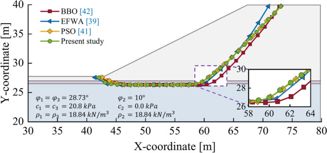
Slope geometry and critical slip surface for benchmark 2.
Table 3.
Comparison of minimum  and standard deviation of EFWA51, Particle swarm optimization53, Biogeography-based optimization54, and present study method for benchmark 2.

In addition, to further explore the distribution of the firefly population during the convergence process and study the convergence behavior of the proposed method, the firefly population distribution was recorded for each iteration and Fig. 9 shows the population distribution at iteration numbers 1, 200, 1000, where the black dots represent the fireflies in the search space. As shown in Fig. 9, the distribution of fireflies in the initial state is relatively decentralized. After 200 iterations, the population gradually moves towards the region for best fitness and the optimal position is continuously refined and updated. Eventually, under the influence of the attraction force, the firefly population converges well, with all individuals becoming evenly distributed around the best position. These results demonstrate that the proposed method exhibits excellent global search capability, robustness, and convergence performance.
Fig. 9.

Firefly search applied to the safety factor function at iteration numbers of (a) 1, (b) 200 and (c) 1000.
Anisotropic slope with bedding plane
The third benchmark involves the stability analysis of an anisotropic geological situation. Referring to the previous work of Ezra3, the associated mechanical parameters are assumed as follows:  10°,
10°,  25 kPa,
  12.5 kN/m3, anisotropy ratio
  0.5 and the height of the slope
  is 20 m. The maximum number of function evaluations
  of FA is set to 500.
In this benchmark, we aim to demonstrate the applicability and accuracy of the proposed method under anisotropic geotechnical conditions. Specifically, we analyze the stability and the shapes of the sliding surfaces depicted in Fig. 10 for various bedding plane angle  of −30, 0, 60, and 90°. In addition, the numerical results of the sliding surface from Ezra3 using the modified log-spiral limit equilibrium (MLSLE) are also plotted for comparison. As shown in Fig. 10, the bedding plane angle has a significant influence on the morphology of the critical sliding surface. With the increase of
  from -30° to 0°, the control point at the top of the slope shifts in the direction of x-coordinate. However, when
  increases from 0 to 60°, this control point moves in the opposite direction. The difference between the results at 60° and 90° is relatively small.
Fig. 10.

Comparison between the locations of the critical slip surfaces determined by the present method with the MLSLE and MLSLE with tension cracks at various bedding plane angle: (a)  −30°, (b)
  0°, (c)
  60°, (d)
  90°.
90°.
Through the conversion of the stability number, the comparative results of the safety factor are presented in (Table 4). From this comparison, it becomes evident that the interaction between the bedding plane angle  and the alignment of the failure geometry significantly affects the value of
  . This effect is most pronounced in (Fig. 10a,c), the maximum and minimum values of
  occur when the failure mechanism is orthogonal to and aligned with
  , respectively. The results obtained by the proposed method are slightly higher than those reported by Ezra3, as shown in (Table 4). The difference may arise from variations in the internal force assumptions or differences in how equilibrium is satisfied in the two methods. However, the trend in the variation of
  remains consistent with the findings in the comparative literature, suggesting that the overall behavior of the system is well captured by our approach. The comprehensive results indicate that the proposed method is both highly applicable and accurate, providing reliable predictions of slope stability under anisotropic conditions.
Table 4.


Numerical results and discussions
The comparative experiments above demonstrate the reliability, stability, and applicability of the method proposed in this study under different conditions. In this section, we investigate the influence of anisotropic shear strength on slope stability by varying three key parameters: the slope angle  , the bedding plane angle
  and the anisotropy ratio
  . Since anisotropy in rock and soil strength parameters significantly affects slope stability3,55, both cohesion anisotropy and frictional anisotropy are considered. The deterministic parameters of the numerical model are set as follows:
  is 12°,
  is 40 kPa,
  is 12 kN/m3, and
  is 20 m.
In the parametric study,  is varied from 35° to 90° in increments of 5°,
  is varied from 0° to 180° in increments of 5° and
  is varied from 0.6 to 1 in increments of 0.1. Note that when
  1, the intensity parameter is isotropic. To further elucidate the effects of anisotropy on slope stability and failure mechanisms, the following numerical model case is analyzed based on the method proposed in this study.
Effect of slope angle
The slope angle  significantly influences both the stability of a slope and its mode of failure. In this study, slope stability is represented by
  , and the classification of slope failure modes follows the approach proposed by Cheng56. Hicks57 defined the sliding depth as the vertical distance from the slope’s apex to the base of the sliding surface. Building upon this definition, Cheng categorized slope failure into three distinct patterns based on the relative relationship between sliding depth and toe height.
Figure 11 shows the critical sliding surfaces for slope angles  of 90, 60, 50 and 35° with a fixed
  of 0°. It can be observed from Fig. 10 that, as the slope angle decreases, the depth of the critical sliding surface increases progressively. Correspondingly, the slope failure mode shifts from shallow failure to deeper failure. From the perspective of slope stability, a general increase in stability is observed as
  decreases. Moreover, comparing the critical slip surfaces at the same slope angle but varying anisotropy ratios reveals that lower horizontal shear strength (i.e., a smaller
  ) leads to a deeper critical failure surface.
Fig. 11.

Anisotropic failure mechanism of slope in a two-layer soil with different  at
at  0° (a):
  90°, (c):
 60°, (b):
  50°, (d):
  35°.
35°.
Figure 12 illustrates the relationship between  and
and  when
when  is fixed at 0°. The results indicate that steeper slopes are more prone to instability. In particular,
  decreases continuously as
  increases between 35 and 45° and again between 60° and 90°. Among these ranges,
  is more sensitive to changes in
  between 35 and 45°. When
  is between 45 and 60°,
  remains relatively constant, showing only slight variations.
Fig. 12.

Function relation between  and
and  when
when  0°.
0°.
Hicks57 noted that slope steepness affects the failure mode and identified 53° as the threshold angle separating shallow from deep sliding modes. As shown in Fig. 12, the results of this study are generally consistent with that observation. According to the calculations from the slope stability analysis program used here, within the range of 35 to 45°, the critical slip surface is relatively deep, indicating a deep failure mode. From 45 to 60°, the slip depth is closer to the slope toe, suggesting an intermediate failure mode. For slopes with angles from 60 to 90°, the slip depth occurs above the toe of the slope, indicating a shallow failure mode.
Additionally, the anisotropy ratio  significantly influences the factor of safety. As
  decreases from 1.0 (isotropic) to 0.6, the degree of anisotropy in geotechnical materials increases, exerting a greater effect on slope stability. For instance, when
  is approximately 40°, reducing
  from 1.0 to 0.6 causes
  to drop from 1.47 to 1.02, a reduction of about 30%. In contrast, when
  is 90°, lowering
  from 1.0 to 0.6 only decreases
  from 0.82 to 0.71, roughly a 13% reduction. These findings indicate that gentler slopes are more sensitive to variations in strength anisotropy than steeper slopes.
Effect of bedding plane angle
The bedding plane angle  plays a critical role in slope stability. Cho4 demonstrated that variations in anisotropic shear strength distribution significantly influence slope behavior, highlighting the importance of incorporating anisotropy into stability analyses. Figure 13 presents the critical sliding surfaces and their corresponding safety factors for different bedding plane angles at
  = 80° with
  values of 0.6 and 1.0. The results indicate that when the critical sliding surface is either perpendicular or parallel to the bedding plane direction, the slope exhibits its lowest or highest stability (Fig. 13b,d), especially the
  of 45 and 135°.
Fig. 13.

Distribution of slip surfaces under different bedding plane angle: (a)  0°, (b)
  45°, (c)
  90°, (d)
  135°, when
  80°.
80°.
At maximum slope stability ( 135°), the factor of safety reaches 0.9314, and both the critical sliding surface and
  closely resemble those observed under isotropic conditions. In contrast, when slope stability is minimized (
 45°), the sliding surface aligns more closely with the bedding plane angle, yielding an
  of 0.6916. Compared to the maximum stability condition,
  decreases by approximately 25.7%.
To further examine the influence of  on slope stability, we analyzed
  as a function of
  under various slope angles (see Fig. 14). As shown in Fig. 14a,
  reaches its minimum near
  = 45° and its maximum near
  = 135°. Although varying
  affects the magnitude of
  , it does not alter the
  angles at which
  attains its minimum or maximum. As
  decreases from 90° to 35°, the
  values corresponding to these extremal
  points shift gradually from 45 and 135 to 15 and 105°, respectively. Figure 14 also illustrates that the impact of strength anisotropy on slope stability becomes more pronounced for gentler slopes. At
  = 90°,
  decreases by up to about 25%, while at
  = 35°, the maximum decrease approaches nearly 31%.
Fig. 14.

 of slope in a two-layer soil under different
  versus the bedding plane angle: (a)
  90°, (b)
  75°, (c)
  50°, (d)
  35°.
35°.
Moreover, the effect of anisotropy ratio  on the maximum
  for a given slope angle is particularly noteworthy. In steep slopes (
 = 90 and 75°), variations in
  have a negligible effect on
  at maximum stability (Fig. 14a,b). In these cases,
  values are similar to those under isotropic conditions. In contrast, as the slope angle decreases, differences in
  at maximum stability become more pronounced across different
  values (Fig. 14c,d). This phenomenon can be attributed to changes in the failure mode. As the failure mode transitions from shallow to deep, the spatial relationship between the failure surface and
  shifts from a simple orthogonal or aligned orientation to a more complex arrangement. Consequently, the
  values corresponding to different
  values, initially nearly identical, diverge as the slope reaches maximum stability.
Figure 15 illustrates the functional relationship between  and
and  under different anisotropy ratios. Specifically, Fig. 15a presents the results for
  = 0.6. By comparing the curves with different
  , it is evident that anisotropy has a relatively greater impact on gentler slopes. Additionally, when examining the
  corresponding to the peak factor of safety
  at various slope angles, it becomes clear that as
  decreases, the
  associated with the peak
  also decreases.
Fig. 15.

 of slope in a two-layer soil under anisotropy ratio
  versus the bedding plane angle: (a)
  0.6, (b)
  0.7, (c)
  0.8, (d)
  0.9.
0.9.
Comparing Fig. 15a,d reveals that a smaller anisotropy ratio  leads to a greater influence of anisotropy on slope stability. Notably, the curves depicting the relationship between bedding plane angles and the factor of safety for
  = 45° and
  = 60° exhibit different trends. Overall,
  shows a gradual increasing trend as
  decreases. However, the changes in
  are relatively subtle for
  = 45° and
  = 60°, which is consistent with the trends observed in (Fig. 12).
When combined with the analysis in Fig. 11 regarding changes in slope failure patterns, the results in Fig. 15 further emphasize that alterations in failure patterns significantly impact slope stability. While the influences of  and
and  on slope stability generally follow a consistent pattern, within certain slope angle ranges (45 to 60°), anisotropy can have a complex and critical effect on slope stability.
Based on the numerical model shown in (Fig. 13a) ( 80°,
80°,  0°), we further investigated the impact of lower anisotropy ratios (
 0.5, 0.4, 0.3, 0.2, and 0.1) on slope stability and obtained some meaningful results. Figure 16 presents the corresponding safety factors and critical slip surfaces distributions for different
  values. The study indicates that as
  gradually decreases, the
  consistently declines at an accelerating rate. Additionally, the spatial distribution of the critical slip surface exhibits notable variations with changes in
  : as
: as  decreases, the critical slip surface expands in the direction away from the slope, and the rate of expansion continuously increases. Nevertheless, given the exceedingly low likelihood of encountering such extreme
  values in practical engineering applications, this paper does not provide an in-depth and systematic analysis of the influence mechanism of extreme
  values on slope stability.
Fig. 16.
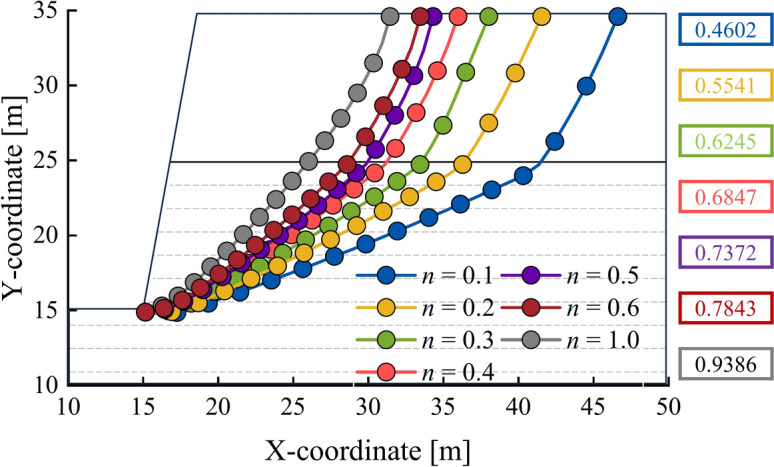
Distribution of critical slip surfaces for different  (
( =80°,
=80°,  =0°).
=0°).
Conclusions
This study introduces a novel method for identifying the critical slip surface of heterogeneous slopes by incorporating the anisotropic yield criterion into the limit equilibrium approach. This method refines the limit equilibrium conditions to fully account for the influence of anisotropic shear strength parameters on slope stability by integrating an anisotropic yield criterion. Numerical benchmarks, including slope in a single soil layer, slope with weak interlayer and anisotropic slope with bedding plane, highlight our model’s ability to capture weak interlayer features and anisotropic characteristics. Numerical convergence studies are also conducted to demonstrate the robustness and reliability of our method.
Additionally, we apply the proposed method to investigate the underlying mechanisms of slope failure under various anisotropic conditions. The results indicate that slopes with anisotropic characteristics generally exhibit lower stability compared to those evaluated under isotropic assumptions. Notably, failure tends to initiate along the direction of minimal shear strength relative to the layering orientation—a trend that is particularly pronounced in steep slopes or in cases of shallow failure modes. A lower anisotropy ratio signifies a higher degree of anisotropy, thereby intensifying its impact on slope stability. This effect is particularly pronounced for slopes with lower gradients, where the anisotropy ratio can lead to a safety factor reduction of up to 31%. Moreover, when the slip surface is orthogonal or parallel to  , the safety factor reaches its maximum or minimum, with these extremes becoming more pronounced as the slope angle decreases. These findings highlight the critical importance of accounting for anisotropic properties in slope stability assessments, especially in environments with complex geological layering and varying slope angles. For future research, we plan to extend this method to three-dimensional analyses and assess its applicability under more complex engineering conditions, such as seismic activity, seepage, external loads, and other factors.
Acknowledgements
This work was financially supported by the National Science Fund for Distinguished Young Scholars (Grant No. 52225403), the National Natural Science Foundation of China (Grant No. 52104089), the National Key Research and Development Program of China (Grant No. 2023YFF0615400), the Shandong Provincial Natural Science Foundation (Grant No. ZR2022QD102) and Demonstration Project of Benefiting People with Science and Technology of Qingdao, China (23-2-8-cspz-13-nsh).
Author contributions
Yongjun Zhang: Methodology, Writing—review & editing. Zhenfu Zhang: Methodology, Writing—original draft, Visualization. Sijia Liu: Supervision, Conceptualization. Mingzhong Gao: Supervision, Resources. Fei Liu: Supervision, Methodology. Jintao Wang: Investigation, Funding acquisition.
Data availability
The data used during the current study is available from the corresponding author on reasonable request.
Declarations
Competing interests
The authors declare no competing interests.
Footnotes
Publisher’s note
Springer Nature remains neutral with regard to jurisdictional claims in published maps and institutional affiliations.
References
- 1.Liu, S., Wang, Y., Peng, C. & Wu, W. A thermodynamically consistent phase field model for mixed-mode fracture in rock-like materials. Comput. Methods Appl. Mech. Eng.392, 114642 (2022). [Google Scholar]
- 2.Liu, S., Kou, M., Wang, Z., Zhang, Y. & Liu, F. A phase-field model for blasting-induced failure and breakage analysis in rock masses. Int. J. Rock Mech. Min. Sci.177, 105734 (2024). [Google Scholar]
- 3.Stockton, E., Leshchinsky, B. A., Olsen, M. J. & Evans, T. M. Influence of both anisotropic friction and cohesion on the formation of tension cracks and stability of slopes. Eng. Geol.249, 31–44 (2019). [Google Scholar]
- 4.Cho, S. E. Effects of spatial variability of soil properties on slope stability. Eng. Geol.92 (3–4), 97–109 (2007). [Google Scholar]
- 5.Tan, X. et al. In-situ direct shear test and numerical simulation of slate structural planes with thick muddy interlayer along bedding slope. Int. J. Rock Mech. Min. Sci.143, 104791 (2021). [Google Scholar]
- 6.Kumar, A., Sharma, R. K. & Mehta, B. S. Slope stability analysis and mitigation measures for selected landslide sites along NH-205 in Himachal Pradesh India. J. Earth Syst. Sci.129, 135 (2020). [Google Scholar]
- 7.Wang, G., Zhao, B., Wu, B., Zhang, C. & Liu, W. Intelligent prediction of slope stability based on visual exploratory data analysis of 77 in situ cases. Int. J. Min. Sci. Technol.33 (1), 47–59 (2023). [Google Scholar]
- 8.ZainAlabideen, K. & Helal, M. Determination of the safe orientation and dip of a rock slope in an open pit mine in Syria using kinematic analysis. Al-Nahrain J. Eng. Sci.19 (1), 33–45 (2016). [Google Scholar]
- 9.Li, S. H., Luo, X. H. & Wu, L. Z. An improved whale optimization algorithm for locating critical slip surface of slopes. Adv. Eng. Softw.157, 103009 (2021). [Google Scholar]
- 10.Ding, J., Zhou, J., Cai, W. & Zheng, D. A modified hybrid algorithm based on black hole and differential evolution algorithms to search for the critical probabilistic slip surface of slopes. Comput. Geotech.129, 103902 (2021). [Google Scholar]
- 11.Huber, M., Scholtès, L. & Lavé, J. Stability and failure modes of slopes with anisotropic strength: Insights from discrete element models. Geomorphology444, 108946 (2024). [Google Scholar]
- 12.He, Y. et al. Slope stability analysis considering the strength anisotropy of c-φ soil. Sci. Rep.12 (1), 18372 (2022). [DOI] [PMC free article] [PubMed] [Google Scholar]
- 13.Badakhshan, E., Noorzad, A., Vaunat, J. & Veylon, G. A critical-state constitutive model for considering the anisotropy in sandy slopes. Arab. J. Geosci.16 (2), 144 (2023). [Google Scholar]
- 14.Nagendran, S. K. & Mohamad Ismail, M. A. Probabilistic and sensitivity analysis of rock slope using anisotropic material models for planar failures. Geotech. Geol. Eng.39 (3), 1979–1995 (2021). [Google Scholar]
- 15.Griffiths, D. V. & Fenton, G. A. Probabilistic slope stability analysis by finite elements. J. Geotech. Geoenviron. Eng.130 (5), 507–518 (2004). [Google Scholar]
- 16.Wang, B., Liu, L., Li, Y. & Jiang, Q. Reliability analysis of slopes considering spatial variability of soil properties based on efficiently identified representative slip surfaces. J. Rock Mechan. Geotech. Eng.12 (3), 642–655 (2020). [Google Scholar]
- 17.Chen, W. F. Stability of slopes. In Limit Analysis and Soil Plasticity (ed. Chen, W. F.) (Elsevier, 1975). [Google Scholar]
- 18.Zang, M. et al. Experimental study on seismic response and progressive failure characteristics of bedding rock slopes. J. Rock Mechan. Geotech. Eng.14 (5), 1394–1405 (2022). [Google Scholar]
- 19.Fellenius, W. Calculation of the stability of earth dams. In Proc. of the Second Congress on Large Dams 4, 445–463 (1936).
- 20.Bishop, A. W. The use of the slip circle in the stability analysis of slopes. Geotechnique5 (1), 7–17 (1955). [Google Scholar]
- 21.Gao, W. & Ge, S. A comprehensive review of slope stability analysis based on artificial intelligence methods. Expert Syst. Applic.239, 122400 (2023). [Google Scholar]
- 22.Zhou, X. P., Huang, X. C. & Zhao, X. F. Optimization of the critical slip surface of three-dimensional slope by using an improved genetic algorithm. Int. J. Geomech.20 (8), 04020120 (2020). [Google Scholar]
- 23.Li, Y., Liu, C., Wang, L. & Xu, S. Stability analysis of inhomogeneous slopes in unsaturated soils optimized by a genetic algorithm. Int. J. Geomech.22 (9), 04022151 (2022). [Google Scholar]
- 24.Kashani, A. R., Chiong, R., Mirjalili, S. & Gandomi, A. H. Particle swarm optimization variants for solving geotechnical problems: review and comparative analysis. Arch. Computat. Methods Eng.28, 1871–1927 (2021). [Google Scholar]
- 25.Zhu, J. F. & Chen, C. F. Search for circular and noncircular critical slip surfaces in slope stability analysis by hybrid genetic algorithm. J. Central South Univ.21(1), 387–397 (2014). [Google Scholar]
- 26.Li, L. et al. Probabilistic seismic slope stability analysis using swarm response surfaces and rotational Newmark sliding model with primary sliding direction. Comput. Geotech.163, 105754 (2023). [Google Scholar]
- 27.Zhang, L. et al. Stability analysis of unsaturated soil slopes with cracks under rainfall infiltration conditions. Comput. Geotech.165, 105907 (2024). [Google Scholar]
- 28.Deng, D. P. Limit equilibrium solution for the rock slope stability under the coupling effect of the shear dilatancy and strain softening. Int. J. Rock Mech. Min. Sci.134, 104421 (2020). [Google Scholar]
- 29.Al-Karni, A. A. & Al-Shamrani, M. A. Study of the effect of soil anisotropy on slope stability using method of slices. Comput. Geotech.26(2), 83–103 (2000). [Google Scholar]
- 30.Dong, J. J., Tu, C. H., Lee, W. R. & Jheng, Y. J. Effects of hydraulic conductivity/strength anisotropy on the stability of stratified, poorly cemented rock slopes. Comput. Geotech.40, 147–159 (2012). [Google Scholar]
- 31.Foroutan Kalourazi, A., Jamshidi Chenari, R. & Veiskarami, M. Bearing capacity of strip footings adjacent to anisotropic slopes using the lower bound finite element method. Int. J. Geomech.20 (11), 04020213 (2020). [Google Scholar]
- 32.Lai, V. Q., Chenari, R. J., Banyong, R. & Keawsawasvong, S. Undrained stability of opening in underground walls in anisotropic clays. Int. J. Geomech.23 (2), 06022042 (2023). [Google Scholar]
- 33.Izadi, A. & Jamshidi Chenari, R. Three-dimensional finite-element lower bound solutions for lateral limit load of piles embedded in cross-anisotropic clay deposits. Int. J. Geomech.21 (12), 04021234 (2021). [Google Scholar]
- 34.Izadi, A. & Chenari, R. J. Combined load bearing capacity of rigid piles embedded in a cross-anisotropic clay deposit using 3D finite element lower bound. J. Rock Mechan. Geotech. Eng.15 (3), 717–737 (2023). [Google Scholar]
- 35.Pishvari, M. N. et al. Undrained bearing capacity of obliquely-eccentrically loaded shallow foundations overlying a heterogeneous and inherently anisotropic clay deposit. J. Rock Mechan. Geotech. Eng.17 (1), 586–613 (2025). [Google Scholar]
- 36.Vanmarcke, E. H. Reliability of earth slopes. J. Geotech. Eng. Div.103 (11), 1247–1265 (1977). [Google Scholar]
- 37.Gravanis, E., Pantelidis, L. & Griffiths, D. V. An analytical solution in probabilistic rock slope stability assessment based on random fields. Int. J. Rock Mech. Min. Sci.71, 19–24 (2014). [Google Scholar]
- 38.Huang, L., Cheng, Y. M., Leung, Y. F. & Li, L. Influence of rotated anisotropy on slope reliability evaluation using conditional random field. Comput. Geotech.115, 103133 (2019). [Google Scholar]
- 39.Liu, L. L., Xu, Y. B., Zhu, W. Q. & Zhang, J. Effect of copula dependence structure on the failure modes of slopes in spatially variable soils. Comput. Geotech.166, 105959 (2024). [Google Scholar]
- 40.Li, J. Z. et al. Probabilistic analysis of pile-reinforced slopes in spatially variable soils with rotated anisotropy. Comput. Geotech.146, 104744 (2022). [Google Scholar]
- 41.Booker, J. R. & Davis, E. H. A general treatment of plastic anisotropy under conditions of plane strain. J. Mech. Phys. Solids20 (4), 239–250 (1972). [Google Scholar]
- 42.Yuan, R., Yu, H. S., Yang, D. S. & Hu, N. On a fabric evolution law incorporating the effects of b-value. Comput. Geotech.105, 142–154 (2019). [Google Scholar]
- 43.Cheng, Y. M. Location of critical failure surface and some further studies on slope stability analysis. Comput. Geotech.30 (3), 255–267 (2003). [Google Scholar]
- 44.Zhu, D. Y., Lee, C. F., Qian, Q. H. & Chen, G. R. A concise algorithm for computing the factor of safety using the morgenstern price method. Can. Geotech. J.42 (1), 272–278 (2005). [Google Scholar]
- 45.Mafi, R., Javankhoshdel, S., Cami, B., Jamshidi Chenari, R. & Gandomi, A. H. Surface altering optimisation in slope stability analysis with non-circular failure for random limit equilibrium method. Georisk: Assess. Manag. Risk Eng. Syst. Geohazards15 (4), 260–286 (2021). [Google Scholar]
- 46.Gandomi, A. H., Yang, X. S. & Alavi, A. H. Mixed variable structural optimization using firefly algorithm. Comput. Struct.89 (23–24), 2325–2336 (2011). [Google Scholar]
- 47.Yang, X. S. Nature-Inspired Metaheuristic Algorithms (Luniver Press, 2010). [Google Scholar]
- 48.Yamagami, T. Search for critical slip lines in finite element stress fields by dynamic programming. In: Proc. 6th Int. Conf. on Numerical Methods in Geomechanics Innsbruck 1347–1352 (1988).
- 49.Mishra, M., Gunturi, V. R. & Maity, D. Teaching-learning-based optimisation algorithm and its application in capturing critical slip surface in slope stability analysis. Soft. Comput.24 (4), 2969–2982 (2020). [Google Scholar]
- 50.Kashani, A. R., Gandomi, A. H. & Mousavi, M. Imperialistic competitive algorithm: a metaheuristic algorithm for locating the critical slip surface in 2-dimensional soil slopes. Geosci. Front.7 (1), 83–89 (2016). [Google Scholar]
- 51.Xiao, Z., Tian, B. & Lu, X. Locating the critical slip surface in a slope stability analysis by enhanced fireworks algorithm. Clust. Comput.22, 719–729 (2019). [Google Scholar]
- 52.Bolton, H., Heymann, G. & Groenwold, A. Global search for critical failure surface in slope stability analysis. Eng. Optim.35 (1), 51–65 (2003). [Google Scholar]
- 53.Gandomi, A. H., Kashani, A. R., Mousavi, M. & Jalalvandi, M. Slope stability analyzing using recent swarm intelligence techniques. Int. J. Numer. Anal. Meth. Geomech.39 (3), 295–309 (2015). [Google Scholar]
- 54.Gandomi, A. H., Kashani, A. R., Mousavi, M. & Jalalvandi, M. Slope stability analysis using evolutionary optimization techniques. Int. J. Numer. Anal. Meth. Geomech.41 (2), 251–264 (2017). [Google Scholar]
- 55.Tatsuoka, F., Nakamura, S., Huang, C. & Tani, K. Strength anisotropy and shear band direction in plane strain tests of sand. Soils Foundations30 (1), 35–54 (1990). [Google Scholar]
- 56.Cheng, H. Z., Chen, J., Wang, Z. S., Hu, Z. F. & Huang, J. H. Stability analysis of a clay slope accounting for the rotated anisotropy correlation structure. Chin. J. Rock Mech. Eng.36 (S2), 3965–3973 (2017). [Google Scholar]
- 57.Hicks, M. A., Nuttall, J. D. & Chen, J. Influence of heterogeneity on 3D slope reliability and failure consequence. Comput. Geotech.61, 198–208 (2014). [Google Scholar]
Associated Data
This section collects any data citations, data availability statements, or supplementary materials included in this article.
Data Availability Statement
The data used during the current study is available from the corresponding author on reasonable request.