ETSpy: A HyperSpy Extension Package for Electron Tomography Data Processing and Reconstruction

Abstract

Electron tomography is a powerful tool for the three-dimensional characterization of materials at the nano- and atomic-scales. A typical workflow for tomography involves several pre-processing steps that may include spatial binning, image registration, and tilt-axis alignment depending upon the nature of the acquired data. Here we describe the capabilities of a new, open-source software package called ETSpy that builds upon the widely-used HyperSpy package. The basic usage of the software and some specific applications are presented.

Graphical Abstract:

1. Introduction

Electron tomography (ET) is a process whereby a three-dimensional (3D) representation of an object is reconstructed from a series of two-dimensional (2D) projection images in the transmission electron microscope(Rosier and Klug, 1968; Crowther and DeRosier, 1970; Frank, 2006). ET has proven to be a valuable technique in both biological(McEwen and Marko, 2001; Lučić et al., 2005; Downing et al., 2007; Gan and Jensen, 2012; Turk and Baumeister, 2020; Young and Villa, 2023) and materials sciences(Midgley and Weyland, 2003; Weyland and Midgley, 2004; Ziese et al., 2004; Kübel et al., 2005; Midgley and Dunin-Borkowski, 2009; Muller and Ercius, 2009; Grenier et al., 2014). Recent advances in aberration correction have even pushed the spatial resolution to the atomic-scale(Scott et al., 2012; Chen et al., 2013; Xu et al., 2015; Miao et al., 2016; Yang et al., 2017; Zhang et al., 2018; Wang et al., 2020a,b; Yang et al., 2021; Pelz et al., 2022) and have integrated spectroscopic methods such as energy dispersive x-ray (EDX) and electron energy-loss (EELS) spectroscopies with the more traditional bright-field or annular dark-field imaging techniques(Möbus et al., 2003; Gass et al., 2006; Yaguchi et al., 2008; Genc et al., 2013; Goris et al., 2013; Bals et al., 2014; Haberfehlner et al., 2014; Pfannmöller et al., 2015; Goris et al., 2016; Zanaga et al., 2016; Zhong et al., 2017, 2018; Bender et al., 2019; Baumann et al., 2020; Han et al., 2021).

Though the the technique is quite flexible and has many modalities, the basic concept remains the same throughout. In ET, we seek to recover an image of an object, $f_x(y,z)$, from a series of projections collected over a range of angles, $\left.P_x(\theta ,y)\right)$. This can be accomplished in a number of ways, but often begins with the inverse Radon transform $({ℛ}^{𝒯})$ (Radon, 1917) such that:

$$\begin{gathered} {\hat{f}}_n(y,z)={ℛ}^{𝒯}\left(P_n(\theta ,y)\right) \\ \theta \in {\theta }_1,{\theta }_2,{\theta }_3,\dots ,{\theta }_k \\ 0\le n<n_x \end{gathered}$$ (1)

where:

$\theta$ : tilt angle for each projection image

$k$ : number of projection images

$nx$ : number pixels in the horizontal image axis, $x$

$y$ : vertical image axis

For the purposes of this paper and the software package which it describes, it is assumed that the tilt axis of the dataset is horizontal (i.e. parallel to the $x$ direction of the images, see Figure 1). Note that in equation 1, the reconstructed image is given as $\hat{f}$ rather than the true object, $f$. This is a result of the finite tilt increment between projections, artifacts arising from data processing errors, the noise content of the projection data, and, in many cases, a hardware/specimen limit on the portion of the full tilt range (0 to $\pi$) that is accessible.

Figure 1:

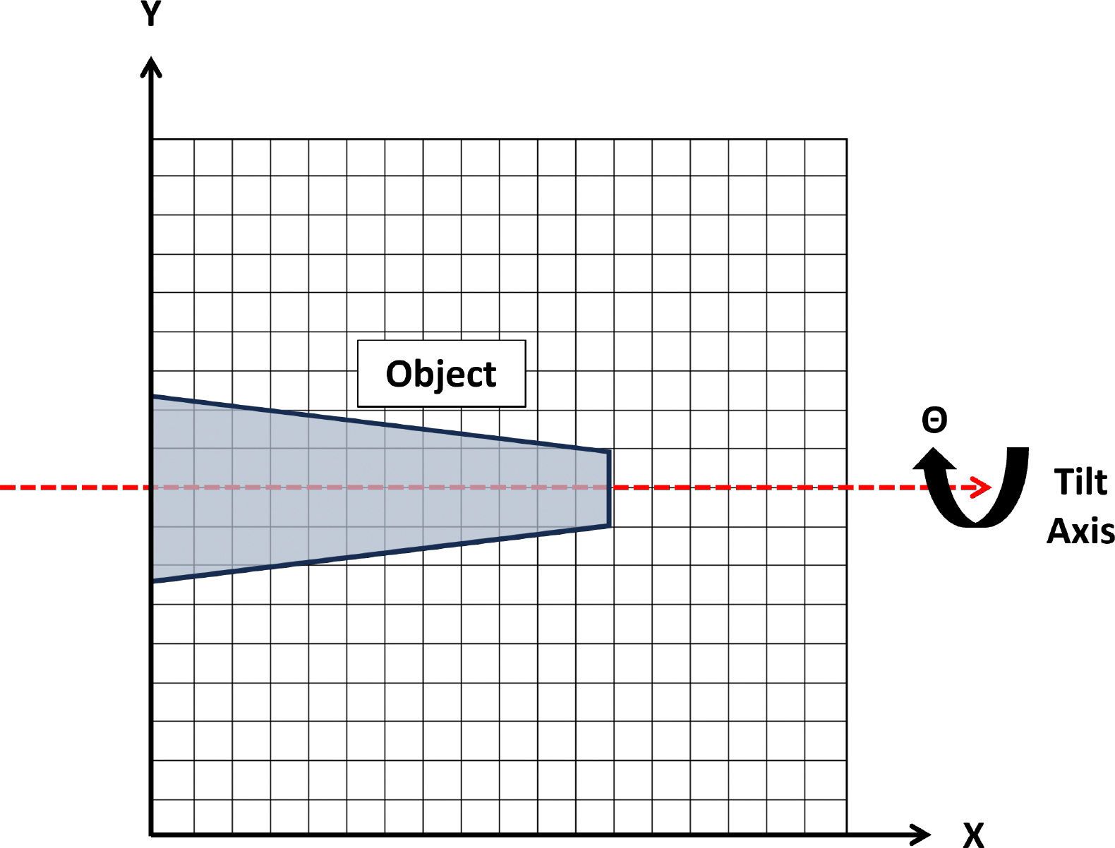
Diagram of the axes convention used in this paper for electron tomography data. The object is rotated about the tilt axis which is parallel to the horizontal axis of the image.

In practice, the workflow begins with the collection of projection images over a range of specimen tilt orientations. At each step, the stage goniometer is advanced by a given tilt increment, one or more new images are collected, and the data is stored for offline processing. If necessary, the stage and/or beam shift can be adjusted after tilting in order to account for mechanical movement of the specimen during tilting and the image can also be refocused. The entire process of tilting, adjusting shifts, focusing, and collecting data can be fully automated, semi-automated, or fully manual. The degree of user interaction that is necessary is typically set by the spatial resolution requirements of the analysis with higher resolution calling for more intervention.

Next, several pre-processing steps can be performed on as needed basis. The full dataset may need to be truncated with some images being discarded due to image quality issues or because the specimen had shifted during acquisition. Often, the dataset will be down-sampled in the spatial domain both to decrease computational requirements in the subsequent steps or to reduce noise. Image filters may also be applied during pre-processing in order to remove noise or image artifacts (e.g. cosmic rays, camera defects, etc.). Prior to reconstruction, the projections must be spatially aligned to a common coordinate system and tilt axis. The former involves the calculation and application of a transformation matrix for each projection in the series, while the latter is accomplished via a global rotation and/or shift of the entire image stack. Failure to either properly register the individual projections to each other or to align the stack to the tilt axis will result in artifacts of varying severity and appearance in the reconstructed volume.

Once pre-processing is complete, the stack is provided as input to a reconstruction algorithm. The goal of the reconstruction process is to convert the input slices along $x$ or the sinograms $\left(P_x(\theta ,y)\right)$ from the tilt series to two-dimensional images of the original object ($f_x(y,z)$). These algorithms fit into two broad classes: analytical methods and iterative methods. The most commonly used analytical method is filtered-backprojection (FBP) which applies a weighting filter to the projections prior to calculating the inverse Radon transform of the projection data (Ramachandran and Lakshminarayanan, 1971). The filter is designed to counteract the blurring effect which results from the finite tilt increment used in acquiring the tilt series data and the non-uniform sampling of the frequency domain this produces. Iterative methods seek to improve upon an initial reconstruction by re-projecting it and comparing to the actual projection data. The two most widely used iterative methods are the simultaneous iterative reconstruction technique (SIRT, (Gilbert, 1972)) and the simultaneous algebraic reconstruction technique (SART, (Andersen and Kak, 1984)). In both cases, the goal is to minimize the difference between the measured projection data and the reprojection of the current reconstruction. In SIRT, the update step is carried out on the full reconstructed image by forward projecting it and comparing to the full input projection data. By contrast, in SART the update step is performed sequentially by forward projecting the current reconstruction estimate for each projection angle and comparing to the input projection data for just that angle. Many other reconstruction methods have been developed more recently for specific applications. These include (among others): (i) the discrete algebraic reconstruction technique (DART, (Batenburg and Sijbers, 2011)) where the the intensity levels in the reconstructed image are iteratively assigned to one of several distinct grayscale values provided by the analyst, (ii) total-variation minimization (TVmin, (Rudin et al., 1992)) which is an iterative method that includes a regularization step to promote smoothness within distinct regions of the image, and (iii) compressed sensing electron tomography (CS-ET, (Saghi et al., 2011)) which produces high-fidelity reconstructions while remaining robust to undersampling conditions in both the spatial and tilt-axis domains.

Finally, the reconstructed volume must be analyzed in some fashion depending on the nature of the features or properties being measured. In some cases, simply visualizing the 3D volume is sufficient to reveal the necessary detail and isosurface generation or volumetric rendering can meet these needs. More often, some features such as interfacial area or the volume fraction of a given phase needs to be measured. To do this, the reconstructed data is typically segmented in some way so each voxel of the tomogram is assigned to a discrete label, allowing for the quantification of various features.

Many software packages, both commercial and open-source, are available for handling some or all of these steps; from data acquisition to pre-processing and on to alignment and eventually reconstruction. It is beyond the scope of this paper to discuss all of these, but, limiting our focus to just the non-commercial open source options, the most widely used package for data acquisition is SerialEM(Mastronarde, 2005, 2024b) which can be paired with the IMOD package(Kremer et al., 1996; Mastronarde, 2024a) for pre-processing, alignment, and reconstruction. Another widely used open-source tool for tomography data processing and visualization is tomviz (Schwartz et al., 2022; tomviz, 2024) which offers a fully developed UI with intuitive workflow options for all stages of the tomography pipeline. Another well-developed open-source option is TomoPy(Gürsoy et al., 2014) which originated for X-ray based tomography work but is readily adapted to ET as well. Finally, a number of plugins for ImageJ, too many to list here, are available, each of which handles some portion of the tomography workflow.

In this paper, we describe the ETSpy package (Herzing, 2024) which is an ET-focused extension of HyperSpy (de la Pena et al., 2017; de la Peña et al., 2024), a popular open-source, Python-based package for the processing of multidimensional data, including electron microscopy and spectroscopy data. ETSpy offers a compact, command line driven interface for pre-processing, alignment, reconstruction, and basic 2D visualization of ET data. Additionally, when used through the Jupyter Notebook or Jupyter Lab interfaces (Beg et al., 2021), ETSpy promotes scientific reproducibility through automatic documentation of all processing steps used to achieve a result. These Jupyter documents can also be easily annotated and shared with collaborators or included alongside any resulting publication. As a HyperSpy extension, ETSpy offers a number of attractive options in terms of the ET workflow. Since the parent package already offers high quality widgets for plotting and visualization of higher dimensional datasets and has embedded a large number of relevant data processing methods, ETSpy can draw on these existing capabilities and the efforts of the large network of active HyperSpy users and developers. In this way, ETSpy joins the growing number of HyperSpy extensions available to analysts all over the world, which as of this publication includes tools for X-ray energy dispersive and electron energy loss spectroscopies(de la Peña et al., 2024), diffraction and 4D-STEM(Johnstone et al., 2024), EBSD(Ånes et al., 2024), cathodoluminescence(Lähnemann et al., 2023), atomic resolution imaging(Nord et al., 2017), holography(Prestat et al., 2024a), and particle analysis(Slater et al., 2021).

2. Test Data

Two test datasets are bundled with ETSpy. These include a simulated tilt series of a catalyst particle consisting of a sphere with small particles of varying size present on the surface and an experimental STEM-HAADF image series collected from a needle-shaped sample from NIST SRM-2135c(NIST, 1999). The latter consists of a silicon substrate with alternating layers of nickel and chromium deposited on the free surface. These datasets can be loaded using the following code:

import etspy.api as etspy
from etspy import datasets as ds

s = ds.get_needle_data() # loads the experimental test data
s2 = ds.get_catalyst_data() # loads the simulated catalyst data

The experimental data is provided in two versions: one which has not been aligned (as it was collected) and another that has already been aligned. The aligned parameter of ds.get_needle_data() controls the version that is loaded (the default is non-aligned):

s = ds.get_needle_data()
s_aligned = ds.get_needle_data(aligned=True)

The model catalyst data (accessed via ds.get_catalyst data()) is fully aligned but misalignment can be applied as the data is read into memory in order to simulate real experimental data. The provided Jupyter notebook uses these datasets to demonstrate the rest of the ETSpy functionality.

3. Signal Classes

Two new Python classes are defined in ETSpy, each of which is a child of HyperSpy’s Signal2D parent class. The first of these new classes is the TomoStack, which contains the tilt series data, metadata, and all of the methods used for data manipulation, alignment, and reconstruction. As in the Signal2D parent class, the TomoStack has navigation axes and signal axes. For an ET image tilt series, the signal axes will be the x and y image axes, while the navigation axis will be the θ tilt angle dimension. The data can be visualized readily using the HyperSpy plot functionality and, when using the Jupyter widget backend for matplotlib (Hunter, 2007), the stack can be interactively viewed in the Jupyter interface as a function of tilt angle.

Relevant metadata for tomographic processing is included in a new node of the standard HyperSpy metadata structure. This metadata can be accessed from the Jupyter command line by typing:

s.metadata.Tomography

and it includes the projection angles, a boolean indicator as to whether or not the data has been previously cropped, the angle of the tilt axis relative to the horizontal axis of the images, and any applied global shifts. The projection angles for the tilt series and the translational shifts of each image are stored as attributes of the TomoStack class as HyperSpy signals. They can be directly accessed as s.tilts and s.shifts, respectively. To view the underlying data values for these signals, the following commands can be used:

s.tilts.data
s.shifts.data

There is an important distinction between the projection angles stored in s.tilts and those referenced in the HyperSpy AxesManager: The values stored in s.tilts are the “true” values used for several alignment processes as well as the reconstruction. The values stored in the HyperSpy AxesManager (which assume a uniform scale between tilts) are used for visualization purposes and should be referenced with caution, as they often may differ from the actual projection angles stored in s.tilts. This distinction allows for arbitrary projections to be removed from a TomoStack via use of the s.remove_projections() method, which is not possible with HyperSpy’s standard axes-handling tools. Future versions of ETSpy may make use of HyperSpy’s ”non-uniform data axis” feature, where the axis values are not evenly spaced, but HyperSpy’s current implementation imposes limitations on other functionality needed for tomographic analysis (such as spatial binning). At the present state, ETSpy will continue to store and use the projection angles in the s.tilts attribute.

In addition to the TomoStack, there is a second class called a RecStack which is used to handle the reconstructed data. At the time of publication, this class mostly provides a way to distinguish between objects containing tilt series data and those containing reconstructed data. It also includes a basic 3D slice plotting function to view images of reconstructed data along the Z-X, Y-X, and Z-Y directions. Additional functionality will be added to this class in the future.

4. Data I/O

ETSpy contains a ‘load’ function for reading data into memory. It can be used in the following ways:

s = tomo.load(“filename.ext”)

image_series = [“image1.ext”, “image2.ext”, “image3.ext”]
s2 = tomo.load(image_series)

Hyperspy (de la Peña et al., 2024) and the associated RosettaSciIO package (Prestat et al., 2024b) already offer robust data reading capabilities for a wide array of ET relevant file formats. ETSpy relies on this functionality to access image data and the required metadata for several formats such as Gatan Digital Micrograph (DM3 or DM4),¹ HDF5 (including the Hyperspy specific HSPY derivative), and MRC. When loaded, HyperSpy reader functions handle the calibration data and ETSpy collects the projection angle data for inclusion with the tilts attribute. Additional ETSpy code is included for handling sets of individual image series in either DM3/DM4 format or MRC/MDOC pairs generated using SerialEM. Finally, if a tilt series already resides in memory as a NumPy array or a HyperSpy Signal2D, it can be directly converted to a TomoStack in the following way:

import etspy.api as etspy
import hyperspy.api as hs
import numpy as np

tilts = np.arange(0,180,2)

s = np.random.random([90,100,100])
s = etspy.TomoStack(s, tilts)

s = hs.signals.Signal2D(np.random.random([90,100,100]))
s = etspy.TomoStack(s, tilts)

Any TomoStack or RecStack can be saved at any point during data processing and analysis. This is done by using the save method and is best accomplished using the HyperSpy hspy format which is a custom version of the HDF5 standard format. When using the hspy format, the data and all of the metadata is stored and easily accessed in the future using the etspy.load method.

5. Basic Visualization

Both the TomoStack and RecStack classes inherit the plotting functionality of the HyperSpy Signal2D class. For example, the code

from etspy import datasets as ds

s = ds.get_catalyst_data()
s.plot()

will load the test catalyst data and plot the first projection image in the stack. When used interactively with ipywidgets a slice navigator can be used to navigate through the stack in the tilt dimension and update the display in real time. By employing the swap_axes method, navigation can also be done over the x-axis which will show the sinogram view. Finally, the TomoStack objcects can be used as input to all other plotting functionality of Hyperspy as well. For example, to compactly plot a projection image alongside a sinogram, the following code can be used:

import hyperspy.api as hs
hs.plot.plot_images([s.inav[0],
                    s.isig[128].as_signal2D([0,1])],
                    colorbar=None)

which produces the output shown in Figure 2.

Figure 2:

Plotting functionality of the TomoStack class shown for the simulated catalyst tilt series. The central projection (left) is shown alongside the central sinogram slice (right).

6. Pre-processing

Spatial sub-sampling can be performed by slicing the signal axes as described in the HyperSpy documentation. In the first line of the code shown below, the result will be to remove the first 5 and last 10 columns and the first 15 and last 20 rows from the input tilt series:

s = ds.get_needle_data()
print(s)
<TomoStack, title: , dimensions: (77|256, 256)>
s_cropped = s.isig [5:−10 , 10:−5]
print(s_cropped)
<TomoStack, title: , dimensions: (77|241, 241)>

The tilt axis can be similarly sliced using the navigation axis of the TomoStack, and the tilts and shifts attributes will be sliced to match:

# each of the following has a navigation size of 77 pixels:
print(s)
<TomoStack, title: , dimensions: (77|256, 256)>
print(s.tilts)
<TomoTilts, title: Image tilt values, dimensions: (77|1)>
print(s.shifts)
<TomoShifts, title: Image shift values, dimensions: (77|2)>

s_cropped = s.inav[5: −10]
# after slicing, each of the following has a navigation size of 62 pixels:
print(s_cropped)
<TomoStack, title: , dimensions: (62|256, 256)>
print(s_cropped.tilts)
<TomoTilts, title: Image tilt values, dimensions: (62|1)>
print(s_cropped.shifts)
<TomoShifts, title: Image shift values, dimensions: (62|2)>

ETSpy also supports removing projections images from the TomoStack in a less uniform way. For example, projections may suffer from irrecoverable alignment or focus issues or otherwise contain artifacts that would degrade the reconstruction quality if included. In that case, a dedicated method named remove_projections() for the TomoStack class has been provided for removal of poor quality projections. For example, imagine that the tenth projection was severely out of focus while in the twentieth projection the sample had drifted too far out of the field of view. The stack can be corrected by removing these images in the following way:

print(s)
<TomoStack, title: , dimensions: (77|256, 256)>

s_new = s.remove_projections([10, 20])
print(s_new)
<TomoStack, title: , dimensions: (75|256, 256)>
print(s_new.tilts)
<TomoTilts, title: Image tilt values, dimensions: (75|1)>
print(s_new.shifts)
<TomoShifts, title: Image shift values, dimensions: (75|2)>

In both cases, the relevant tilt angles are also removed from the tilts and shifts attributes to ensure the relationship between the projection images and the projection angles/shifts is correct. As a word of caution, after using the remove_projections() method, the navigation axis for the signal (s_new.axes_manager[“Projections”]) will no longer be synchronized with the actual tilt values stored in s_new.tilts, due to the limitations described in Section 3.

Filtering of the stack can also be performed using the filter method of the TomoStack class. Currently, Sobel, median, and band-pass filters are implemented along with a combined median and Sobel option. Additional filters can be easily added or applied directly to the underlying data array of the TomoStack. This can be useful for improving the accuracy of the stack alignment methods. Translational shifts can be calculated on the filtered stack and applied to the unfiltered stack using the align_other method, as discussed below.

7. Image Registration

Multiple options exist for calculating and applying translational shifts for aligning the images of the stack using the register_stack method of the TomoStack class. The available options are:

• Phase correlation (“PC”)

• StackReg (“StackReg”)

• Center of Mass (“COM”)

• Combined center of mass and common line (“COM-CL”)

Phase correlation (PC) (Guizar-Sicairos et al., 2008) analysis, a normalized form of Fourier cross-correlation, is carried out using the scikit-image(Walt et al., 2014) implementation. The StackReg option uses the Python implementation(Lichtner, 2023) of an algorithm first described by Thevenaz et al. (1998) and originally implemented in ImageJ(Thévenaz, 2011). In this method, the transformation is iteratively calculated by minimization of a cost function based on the sum squared difference of intensities between two images. The COM option employs a Python version of a set of algorithms developed by Sanders et al. (2015) which were first implemented in Matlab. The method traces center of mass of the object at several locations along the tilt axis and minimizes the error between the measurements and the path expected for such an object over the set of projection angles that were used for data collection. Finally, the COM-CL option employs a two step alignment first described by Scott et al. (2012). In this case, shifts are first calculated in the direction perpendicular to the tilt axis by center of mass tracking. Then, the shifts parallel to the tilt axis are determined via the common-line method which involves projecting the image along the direction perpendicular to the tilt axis and serially cross-correlating the resulting profiles. All of these methods have advantages and disadvantages. PC is straightforward and fast, although it can be challenged by noisy data, by samples which exhibit regularly repeating features, or when the differences in image features between two images is large (e.g. when a large tilt increment is used). StackReg will often outperform PC in these cases but is computationally more expensive. Finally, both COM and COM-CL incorporate the geometry of the tilt series acquisition and are very effective for particulate or pillar shaped samples since little or no additional material enters the field of view during tilting in these cases. However, they will often fail when slab type specimen geometries are used or when significant amounts of extraneous material enters and leaves the field of view over the course of the series. Further detail about all of these methods can be found in the provided citations.

Regardless of the method chosen, translation shifts are calculated between each set of images in the stack. The shifts are then composed such that they are made relative to the previous shift in the stack starting from a user defined projection number. If the user does not define this starting projection number, the midpoint of the stack is used.

Finally, the shifts can be calculated using any of these methods and then applied to another stack using the align_other method. This approach is useful when multiple image signals are collected during a single tilt series acquisition and when one of the signals has superior characteristics for calculating the alignment shifts compared to another. For example, shifts can be calculated on a high signal-to-noise ratio medium-angle annular dark field (MAADF) image stack and applied to a noisier high-angle annular dark field (HAADF) stack. Since both signals are acquired simultaneously, the shifts for each will be the same. This can also be used to calculate shifts using an image signal collected alongside a hyperspectral EDX or EELS dataset and then apply those shifts to the spectral images extracted from the datacube (see section 10 for more detail).

8. Tilt-axis Alignment

In order ensure that the tilt axis of the dataset is centered and made as close to horizontal as possible prior to reconstruction, a global shift and rotation of the stack can also be calculated and applied using the tilt_align method. Two options are available in this case:

• Center of mass tracking (“COM”)

• Maximum projection image analysis (“MaxImage”)

The first of these is based on a method described by Wolf (2012) and involves tracking the center of mass at multiple locations along the tilt axis and fitting these to the motion expected for an ideal cylinder. This method works very well for pillar- or needle-shaped specimen geometries. Alternatively, the MaxImage method analyzes features in the projected maximum image of a spatially registered stack using a combination of edge-detection and Hough transform analysis in order to determine the tilt axis rotation. This method is particularly effective when particles are present in the sample which trace linear paths in the projected maximum image. Optionally, the global shift of the tilt axis can also be calculated by minimization of the sum of the reconstruction. In both cases, the measured shift and rotation are stored in the Tomography node of the metadata structure and can be applied to other stacks using the align_other method described in the previous section.

An example of the full, automated alignment process is illustrated in Figure 3 which shows the maximum projection images from the simulated catalyst tilt series prior to alignment, after stack registration via “StackReg” and after a tilt axis alignment via the “MaxImage” method. The reconstruction at each stage is also shown with varying artifacts due to misalignment.

Figure 3:

Alignment results. Maximum projection images of the tilt series (top series) are shown for the misaligned stack, the registered stack, and the fully aligned stack along with the resulting reconstructions (SIRT, 100 iterations) from each (bottom row).

Finally, where the automated approaches fail for a particular dataset, a manual approach is also available. This is done using the test_align method which displays three reconstructed sinograms extracted from user-defined locations in the stack. If the user does not define these locations, positions at one quarter, one half, and three quarters of the stack width are chosen. By visual inspection of the features in these reconstructions, it is often possible to iteratively determine the best shift and tilt and tilt values by altering one or both parameters and re-executing test_align multiple times.

9. Reconstruction

There are four reconstruction algorithms currently available in ETSpy and each relies on the ASTRA toolbox (Aarle et al., 2015) to perform the reconstruction. The available options are:

• Simple backprojection (“BP”)

• Filtered backprojection (“FBP”, default)

• Simultaneous iterative reconstruction technique (“SIRT”)

• Simultaneous algebraic reconstruction technique (“SART”)

• Discrete algebraic reconstruction technique (“DART”)

Reconstruction is initiated by calling the reconstruct method of the TomoStack. The ASTRA toolbox offers CPU-based and CUDA-based GPU-accelerated options for the BP, FBP, SIRT, and SART methods. ETSpy will attempt to determine whether a CUDA-compatible GPU is available and use it for faster reconstruction when possible. Alternatively, the reconstruction will be carried out using parallel computation on the CPU using the Python multiprocessing package. The DART implementation employed in ETSpy is based on custom Python code and no CUDA-acceleration is available at the present time. The reconstruction returns a RecStack object which contains the 3D reconstructed image data.

For the iterative SIRT and SART reconstruction methods, another function (recon_error) is provided to perform a reconstruction on a single slice of the tilt series data and return a series of reconstructions showing the progress at each iteration along with a measure of the error at each step. This can be useful in determining the number of iterations to perform on the entire stack. Once completed, the resulting stack can be interactively plotted to see how the reconstructed image changes with iteration. The error is returned as a HyperSpy Signal2D array which can be interrogated numerically or graphically. For CUDA-capable systems, ASTRA offers a way to do this directly using astra.algorithm.get_res_norm. For systems without CUDA, ETSpy will use the numpy.linalg.norm function to calculate the error between the sinogram and the reconstruction at each iteration. An example of this process is shown in 4.

10. Hyperspectral Tomography

To demonstrate the use of ETSpy for processing hyperspectral tomography, data was collected from another needle-shaped sample of the NIST SRM-2135c depth-profiling standard. Several EDX spectrum images (SIs) were collected every 5° over a 180° tilt range using an on-axis style tomography holder (Fischione Model 2050). The data were collected using an EDAX Octane-T silicon drift detector and the acquisition was controlled by the EDAX TEAM software. The SIs were 162 × 128 pixels in size with 3 nm square pixels. The probe current was approximately 0.5 nA and the per pixel dwell time was 200 ms. At each new tilt, the sample was manually aligned to an image at the previous tilt using a combination of beam and stage shifting. The sum spectrum for the entire spectral tomography dataset is shown along with the sum image calculated from a single projection angle in Figure 5.

Figure 5:

Sum spectrum of the fully spectral tomography dataset (top) and sum image extracted from a single spectrum image projection (bottom)

Once acquired, the TEAM SPD files were converted to HDF5 format using Hyperspy. All that remains to utilize ETSpy for reconstructing the chemical maps is to extract the required 2D elemental maps at each tilt and converting each of the resulting HyperSpy Signal2D instances to a TomoStack. Using HyperSpy, this is can be done either via straightforward background subtraction methods, curve fitting or via machine learning algorithms. Examples of background subtraction and the non-negative matrix factorization machine learning algorithm(Paatero and Tapper, 1994) are shown in the following code:

import hyperspy.api as hs
import etspy.api as etspy

# Load EDX datasets and define tilts
edx = hs.load(“EDX_SI_*.hdf5”, reader=‘HSPY’, stack=True)
tilts = np.linspace(0, 180, 37)

## Background Subtraction Method
# Define lines to use and background windows
lines = [‘Si_Ka’, ‘Ni_Ka’, ‘Cr_Ka’,’Pt_La’]
bckg = [[1.2,1.4,3.2,3.4],[4.5,4.8,11.9,12.5],
        [4.5,4.8,11.9,12.5],[4.5,4.8,11.9,12.5]]

# Extract elemental maps
maps = edx.get_lines_intensity(lines,
                               background_windows=bckg)
SiKa, NiKa, CrKa, PtLa = maps

# Convert maps to TomoStack
SiKa = etspy.TomoStack(SiKa, tilts)
NiKa = etspy.TomoStack(NiKa, tilts)
CrKa = etspy.TomoStack(CrKa, tilts)
PtLa = etspy.TomoStack(PtLa, tilts)

## NMF decomposition
# Perform initial singular value decomposition
edx.decomposition(True)
# Refine the decomposition using NMF
edx.decomposition(True,
                  algorithm=“nmf”,
                  output_dimension=6)

# Extract phase maps and convert to TomoStacks
loadings = edx.get_decomposition_loadings()
Ni_NMF = etspy.TomoStack(loadings.inav[0], tilts)
Si_NMF = etspy.TomoStack(loadings.inav[1], tilts)
Cr_NMF = etspy.TomoStack(loadings.inav[2], tilts)
Pt_NMF = etspy.TomoStack(loadings.inav[3], tilts)

Once the TomoStack’s have been created using either method, it is then just a matter of following the usual tomographic work flow of stack registration, tilt-axis alignment and reconstruction. Since the elemental maps are often not well suited for calculating alignment transformations, we can either use a tilt series of an image signal collected simultaneously (e.g. HAADF, etc.) or by the spectral sum images for alignment followed by using the align_other method of the TomoStack to apply the calculated alignment to each spectral tilt series. The latter option using the spectral sum image is shown below:

## Calculate alignment on the spectral sum image series

# Calculate sum image. This results in a HyperSpy
# Signal2D class
edx_sum = edx.sum(3).as_signal2D((0,1))

# Convert to a TomoStack
edx_sum = etspy.TomoStack(si_sum, tilts)

edx_reg = edx_sum.stack_register(‘StackReg’)
edx_ali = edx_reg.tilt_align(‘CoM’)

# Apply alignments to the phase maps
Ni_NMF = edx_ali.align_other(Ni_NMF)
Si_NMF = edx_ali.align_other(Si_NMF)
Cr_NMF = edx_ali.align_other(Cr_NMF)
Pt_NMF = edx_ali.align_other(Pt_NMF)

# Reconstruct the datasets
Ni_rec = Ni_NMF.reconstruct()
Si_rec = Si_NMF.reconstruct()
Cr_rec = Cr_NMF.reconstruct()
Pt_rec = Pt_NMF.reconstruct()

The component images produced by the NMF decomposition for one projection of the full hyperspectral tomography dataset are shown in Figure 6. In this case, the first four components show the spatial distribution of the nickel, silicon, chromium, and platinum signals, respectively. Components five and six (not shown), were related to the absorption of the nickel and chromium L-lines.

Figure 6:

Results of NMF decomposition of spectral tomography dataset. Components 1 through 4 are shown along with a color overlay emphasizing their spatial extent.

Since the data underlying these images was collected simultaneously with that which is used to generate the sum images described previously, the alignments calculated in the latter case can also be applied here. Finally, the individual NMF image series are reconstructed independently and slices from each are displayed in Figure 7.

Figure 7:

Slices extracted from reconstructions of the NMF components associated with nickel (top), chromium (middle), and silicon (bottom)

At this point, the reconstructions can be quantified using packages such as NumPy, SciPy, scikit-image, etc., all of which can be accessed directly from the same Jupyter Notebook used for ETSpy processing. For example, it is very straigtforward to binarize the reconstructions of the nickel and chromium layers and calculate volumetric ratios of each:

pixel_size = Ni_rec.axes_manager[0].scale
Ni_binary = Ni_rec.deepcopy()
Ni_binary[Ni_binary>0] = 1

Cr_binary = Cr_rec.deepcopy()
Cr_binary[Cr_binary>0] = 1

Ni_volume = pixel_size**3 * Ni_binary.sum()
Cr_volume = pixel_size**3 * Cr_binary.sum()

volume_ratio = Ni_volume/Cr_volume

This is just one simple example to illustrate the way in which tomographic reconstructions generated using ETSpy can be directly interrogated within the Jupyter environment.

Finally, 3D visualization can be carried out in one of two ways. First, the reconstructions can be saved to disk and then read into dedicated visualization software. Alternatively, for those who wish to remain in the Python environment used for the rest of the data processing, packages such as ipyvolume or mayavi can be used from some basic visualization. An example of using ipyvolume is shown in Figure 8.

Figure 8:

Volumetric rendering using ipyvolume of the Cr-K_α, Ni-K_α, and Si-K_α tomographic reconstructions (red, green, and blue, respectively).

11. Conclusions

In this paper, we have described the ETSpy software package, a new Hyperspy extension that is specifically tailored to enhance the processing and reconstruction of electron tomography data. The package provides a comprehensive suite of tools designed to streamline the workflow from data input to final reconstruction.

The package leverages the already powerful capabilities of its parent package and adds a host of application specific functionality for electron tomography data. This includes data pre-processing, image registration, tilt axis alignment, 3D reconstruction, and basic visualization. Since it is Python-based, the package is easily scriptable and when used within the Jupyter Lab interface can be thoroughly documented and easily shared. The combination of HyperSpy’s core functionality with the new capabilities of ETSpy is most apparent in the processing of hyperspectral tomography datasets since initial tasks such as background subtraction and machine learning decomposition are seamlessly integrated with tomographic alignment and reconstruction.

Figure 4:

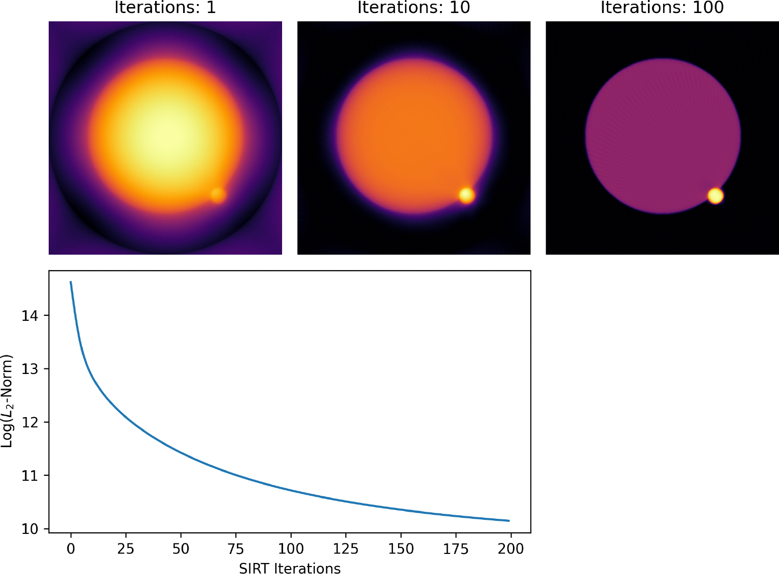
Iterative reconstruction convergence analysis. Reconstructed slice from the simulated catalyst tilt series shown after an increasing number of SIRT iterations (top row). Also shown is the L₂-norm of the difference between the reconstruction and the input projection data (log scale) as a function of SIRT iteration (bottom).

Highlights.

• Open-source software for pre-processing and reconstruction of electron tomography data

• Implemented as an extension of the HyperSpy library, providing data visualization, machine learning, and spectrum image processing functionalities

• A seamless package for pre-processing and tomographic reconstruction that can easily be run via scripts or through Jupyter Notebooks for interactive development, ease of sharing, and inline documentation

Appendix A. Code and Data Availability

The ETSpy package is hosted on GitHub under the usnistgov organization: https://github.com/usnistgov/ETSpy and can be cited using the following DOI: https://doi.org/10.18434/mds2-3616. Extensive documentation is available at the project’s homepage: https://pages.nist.gov/etspy. In addition to the code itself, a Jupyter notebook is provided to demonstrate the basic functionality described in this paper, which should be available at https://pages.nist.gov/etspy/examples/etspy_demo.html (in the event that link changes, it is also available from the GitHub repository).

The EDX tomography dataset can be accessed at : https://doi.org/10.18434/mds2-3631.

Appendix B. Package Installation

Due to the integration of compiled and GPU-accelerated features, installation is most easily accomplished by using Anaconda(Anaconda Software Distribution) to create a new environment and to install the package from the conda-forge repository:

conda create -n etspy
conda activate etspy
conda install -c conda-forge etspy

References

- Aarle W.v., Palenstijn WJ, Beenhouwer JD, Altantzis T, Bals S, Batenburg KJ, Sijbers J, 2015. The ASTRA Toolbox: A platform for advanced algorithm development in electron tomography. Ultramicroscopy 157, 35–47. doi: 10.1016/j.ultramic.2015.05.002. [DOI] [PubMed] [Google Scholar]
- Anaconda Software Distribution, 2024. URL: https://docs.anaconda.com/. accessed: 2024-07-11. [Google Scholar]
- Andersen AH, Kak AC, 1984. Simultaneous algebraic reconstruction technique (sart): A superior implementation of the art algorithm. Ultrasonic Imaging 6, 81–94. doi: 10.1016/0161-7346(84)90008-7. [DOI] [PubMed] [Google Scholar]
- Ånes HW, Lervik LAH, Natlandsmyr O, Bergh T, Prestat E, Bugten AV, Østvold EM, Xu Z, Francis C, Nord M, 2024. Pyxem/kikuchipy: Kikuchipy 0.10.0 . Zenodo. doi: 10.5281/zenodo.11432173. [DOI] [Google Scholar]
- Bals S, Goris B, Liz-Marzán LM, Van Tendeloo G, 2014. Three-Dimensional Characterization of Noble-Metal Nanoparticles and their Assemblies by Electron Tomography. Angewandte Chemie International Edition 53, 10600–10610. doi: 10.1002/anie.201401059. [DOI] [PubMed] [Google Scholar]
- Batenburg KJ, Sijbers J, 2011. DART: A Practical Reconstruction Algorithm for Discrete Tomography. IEEE Transactions on Image Processing 20, 2542–2553. doi: 10.1109/tip.2011.2131661. [DOI] [PubMed] [Google Scholar]
- Baumann FH, Popielarski B, Lu Y, Mitchell T, 2020. Extension of CD-TEM Towards 3D Elemental Mapping. IEEE Transactions on Semiconductor Manufacturing 33, 346–351. doi: 10.1109/TSM.2020.2990588. conference Name: IEEE Transactions on Semiconductor Manufacturing. [DOI] [Google Scholar]
- Beg M, Taka J, Kluyver T, Konovalov A, Ragan-Kelley M, Thiéry NM, Fangohr H, 2021. Using jupyter for reproducible scientific workflows. Computing in Science & Engineering 23, 36–46. doi: 10.1109/MCSE.2021.3052101. [DOI] [Google Scholar]
- Bender H, Richard O, Kundu P, Favia P, Zhong Z, Palenstijn WJ, Batenburg KJ, Wirix M, Kohr H, Schoenmakers R, 2019. Combined STEM-EDS tomography of nanowire structures. Semiconductor Science and Technology 34, 114002. doi: 10.1088/1361-6641/ab4840. [DOI] [Google Scholar]
- Chen CC, Zhu C, White ER, Chiu CY, Scott MC, Regan BC, Marks LD, Huang Y, Miao J, 2013. Three-dimensional imaging of dislocations in a nanoparticle at atomic resolution. Nature 496, 74–77. doi: 10.1038/nature12009. [DOI] [PubMed] [Google Scholar]
- Crowther R, DeRosier D, 1970. The reconstruction of a three-dimensional structure from projections and its application to electron microscopy. Proceedings of the Royal Society A 317, 319–340. doi: 10.1098/rspa.1970.0119. [DOI] [PubMed] [Google Scholar]
- de la Peña F, Prestat E, Burdet P, Lähnemann J, MacArthur KE, Fauske VT, Sarahan M, Francis C, Johnstone DN, Ostasevicius T, Migunov V, Furnival T, Nord M, Mazzucco S, Eljarrat A, Caron J, Aarholt T, Poon T, Jokubauskas P, actions-user, Winkler F, Taillon J, Slater T. pquinn-dls,, Guzzinati G, Myers JC, Tappy N, Garmannslund A, 2024. Hyperspy/exspy: V0.2. Zenodo. doi: 10.5281/zenodo.10953535. [DOI] [Google Scholar]
- Downing KH, Sui H, Auer M, 2007. Electron tomography: a 3d view of the subcellular world. Analytical chemistry 79, 7949–57. doi: 10.1021/ac071982u. [DOI] [PubMed] [Google Scholar]
- Frank J, 2006. Electron Tomography. Springer, New York. doi: 10.1007/978-0-387-69008-7. [DOI] [Google Scholar]
- Gan L, Jensen GJ, 2012. Electron tomography of cells. Quarterly Reviews of Biophysics 45, 27–56. doi: 10.1017/S0033583511000102. [DOI] [PMC free article] [PubMed] [Google Scholar]
- Gass MH, Koziol KK, Windle AH, Midgley PA, 2006. Four-dimensional spectral tomography of carbonaceous nanocomposites. Nano letters 6, 376–9. doi: 10.1021/nl052120g. [DOI] [PubMed] [Google Scholar]
- Genc A, Kovarik L, Gu M, Cheng H, Plachinda P, Pullan L, Freitag B, Wang C, 2013. XEDS STEM tomography for 3D chemical characterization of nanoscale particles. Ultramicroscopy 131, 24–32. doi: 10.1016/j.ultramic.2013.03.023. [DOI] [PubMed] [Google Scholar]
- Gilbert P, 1972. Iterative methods for the three-dimensional reconstruction of an object from projections. Journal of theoretical biology 36, 105–17. doi: 10.1016/0022-5193(72)90180-4. [DOI] [PubMed] [Google Scholar]
- Goris B, Backer A, Aert S, Gómez-Graña S, Liz-Marzán LM, Tendeloo G, Bals S, 2013. Three-Dimensional Elemental Mapping at the Atomic Scale in Bimetallic Nanocrystals. Nano Letters 13, 4236–4241. doi: 10.1021/nl401945b. [DOI] [PubMed] [Google Scholar]
- Goris B, Meledina M, Turner S, Zhong Z, Batenburg KJ, Bals S, 2016. Three dimensional mapping of Fe dopants in ceria nanocrystals using direct spectroscopic electron tomography. Ultramicroscopy 171, 55–62. doi: 10.1016/j.ultramic.2016.08.017. [DOI] [PubMed] [Google Scholar]
- Grenier A, Duguay S, Barnes J, Serra R, Haberfehlner G, Cooper D, Bertin F, Barraud S, Audoit G, Arnoldi L, Cadel E, Chabli A, Vurpillot F, 2014. 3d analysis of advanced nano-devices using electron and atom probe tomography. Ultramicroscopy 136, 185–192. doi: 10.1016/j.ultramic.2013.10.001. [DOI] [PubMed] [Google Scholar]
- Guizar-Sicairos M, Thurman ST, Fienup JR, 2008. Efficient subpixel image registration algorithms. Opt. Lett. 33, 156–158. doi: 10.1364/OL.33.000156. [DOI] [PubMed] [Google Scholar]
- Gürsoy D, De Carlo F, Xiao X, Jacobsen C, 2014. TomoPy: A framework for the analysis of synchrotron tomographic data. Journal of Synchrotron Radiation 21, 1188–1193. doi: 10.1107/S1600577514013939. [DOI] [PMC free article] [PubMed] [Google Scholar]
- Haberfehlner G, Orthacker A, Albu M, Li J, Kothleitner G, 2014. Nanoscale voxel spectroscopy by simultaneous EELS and EDS tomography. Nanoscale 6, 14563–14569. doi: 10.1039/c4nr04553j. [DOI] [PubMed] [Google Scholar]
- Han Y, Jang J, Cha E, Lee J, Chung H, Jeong M, Kim TG, Chae BG, Kim HG, Jun S, Hwang S, Lee E, Ye JC, 2021. Deep learning STEM-EDX tomography of nanocrystals. Nature Machine Intelligence 3, 267–274. doi: 10.1038/s42256-020-00289-5. [DOI] [Google Scholar]
- Herzing A, 2024. usnistgov/etspy: ETSpy package URL: https://github.com/usnistgov/etspy. [Google Scholar]
- Hunter JD, 2007. Matplotlib: A 2d graphics environment. Computing in Science & Engineering 9, 90–95. doi: 10.1109/MCSE.2007.55. [DOI] [Google Scholar]
- Johnstone D, Crout P, Francis C, Nord M, Laulainen J, Høgås S, Opheim E, Prestat E, Martineau B, Bergh T, Cautaerts N, Ånes HW, Smeets S, Femoen VJ, Ross A, Broussard J, Huang S, Collins S, Furnival T, Jannis D, Hjorth I, Jacobsen E, Danaie M, Herzing A, Poon T, Dagenborg S, Bjørge R, Iqbal A, Morzy J, Doherty T, Ostasevicius T, Thorsen TI, von Lany M, Tovey R, Vacek P, 2024. Pyxem/pyxem: V0.19.1. Zenodo. doi: 10.5281/zenodo.11585254. [DOI] [Google Scholar]
- Kremer JR, Mastronarde DN, McIntosh J, 1996. Computer Visualization of Three-Dimensional Image Data Using IMOD. Journal of Structural Biology 116, 71–76. doi: 10.1006/jsbi.1996.0013. [DOI] [PubMed] [Google Scholar]
- Kübel C, Voigt A, Schoenmakers R, Otten M, Su D, Lee TC, Carlsson A, Bradley J, 2005. Recent advances in electron tomography: TEM and HAADF-STEM tomography for materials science and semiconductor applications. Microscopy and Microanalysis 11, 378–400. doi: 10.1017/s1431927605050361. [DOI] [PubMed] [Google Scholar]
- Lähnemann J, Orri JF, Prestat E, Ånes HW, Johnstone DN, Migrator LGTM., Tappy N, 2023. LumiSpy/lumispy: V0.2.2. Zenodo. doi: 10.5281/zenodo.7747350. [DOI] [Google Scholar]
- Lichtner G, 2023. Pystackreg github repository. URL: https://github.com/glichtner/pystackreg. [Google Scholar]
- Lučić V, Förster F, Baumeister W, 2005. Structural Studies by Electron Tomography: From Cells to Molecules. Annual Review of Biochemistry 74, 833–865. doi: 10.1146/annurev.biochem.73.011303.074112. [DOI] [PubMed] [Google Scholar]
- Mastronarde DN, 2005. Automated electron microscope tomography using robust prediction of specimen movements. Journal of Structural Biology 152, 36–51. doi: 10.1016/j.jsb.2005.07.007. [DOI] [PubMed] [Google Scholar]
- Mastronarde DN, 2024a. Imod: Image processing and 3d reconstruction. URL: https://bio3d.colorado.edu/imod/. [Google Scholar]
- Mastronarde DN, 2024b. Serialem: A program for automated electron microscope tomography. URL: https://bio3d.colorado.edu/SerialEM/index.html. [Google Scholar]
- McEwen BF, Marko M, 2001. The Emergence of Electron Tomography as an Important Tool for Investigating Cellular Ultrastructure. Journal of Histochemistry & Cytochemistry 49, 553–563. doi: 10.1177/002215540104900502. [DOI] [PubMed] [Google Scholar]
- Miao J, Ercius P, Billinge SJL, 2016. Atomic electron tomography: 3d structures without crystals. Science 353, aaf2157. doi: 10.1126/science.aaf2157. [DOI] [PubMed] [Google Scholar]
- Midgley P, Weyland M, 2003. 3d electron microscopy in the physical sciences: the development of z-contrast and EFTEM tomography. Ultramicroscopy 96, 413–431. doi: 10.1016/s0304-3991(03)00105-0. [DOI] [PubMed] [Google Scholar]
- Midgley PA, Dunin-Borkowski RE, 2009. Electron tomography and holography in materials science. Nature Materials 8. doi: 10.1038/nmat2406. [DOI] [PubMed] [Google Scholar]
- Muller D, Ercius P, 2009. Electron tomography in materials science. Microscopy and Microanalysis 15, 1534–1535. doi: 10.1017/s1431927609098262. [DOI] [PubMed] [Google Scholar]
- Möbus G, Doole RC, Inkson BJ, 2003. Spectroscopic electron tomography. Ultramicroscopy 96, 433–451. doi: 10.1016/s0304-3991(03)00106-2. [DOI] [PubMed] [Google Scholar]
- NIST, 1999. NIST SRM 2135c Certificate of Analysis Ni/Cr Thin Film Depth Profile Standard. Technical Report National Institute of Standards and Technology. Gaithersburg, MD USA. [Google Scholar]
- Nord M, Vullum PE, MacLaren I, Tybell T, Holmestad R, 2017. Atomap: A new software tool for the automated analysis of atomic resolution images using two-dimensional Gaussian fitting. Advanced Structural and Chemical Imaging 3, 9. doi: 10.1186/s40679-017-0042-5. [DOI] [PMC free article] [PubMed] [Google Scholar]
- Paatero P, Tapper U, 1994. Positive matrix factorization: A non-negative factor model with optimal utilization of error estimates of data values. Environmetrics 5, 111–126. doi: 10.1002/env.3170050203. [DOI] [Google Scholar]
- Pelz PM, Groschner C, Bruefach A, Satariano A, Ophus C, Scott MC, 2022. Simultaneous successive twinning captured by atomic electron tomography. ACS Nano 16, 588–596. doi: 10.1021/acsnano.1c07772. publisher: American Chemical Society. [DOI] [PubMed] [Google Scholar]
- de la Pena F, Ostasevicius T, Tonaas Fauske V, Burdet P, Jokubauskas P, Nord M, Sarahan M, Prestat E, Johnstone DN, Taillon J, et al. , 2017. Electron microscopy (big and small) data analysis with the open source software package HyperSpy. Microscopy and Microanalysis 23, 214–215. doi: 10.1017/S1431927617001751. [DOI] [Google Scholar]
- de la Peña F, Prestat E, Fauske VT, Lähnemann J, Burdet P, Jokubauskas P, Furnival T, Francis C, Nord M, Ostasevicius T, MacArthur KE, Johnstone DN, Sarahan M, Taillon J, Aarholt T, pquinn dls, Migunov V, Eljarrat A, Caron, Nemoto T, Poon T, Mazzucco S, actions user, Tappy N, Cautaerts N, Somnath S, Slater, Walls M, pietsjoh, Ramsden H, 2024. Hyperspy. doi: 10.5281/zenodo.11148112. [DOI] [Google Scholar]
- Pfannmöller M, Heidari H, Nanson L, Lozman O, Chrapa M, Offermans T, Nisato G, Bals S, 2015. Quantitative Tomography of Organic Photovoltaic Blends at the Nanoscale. Nano Letters 15, 6634–42. doi: 10.1021/acs.nanolett.5b02437. [DOI] [PubMed] [Google Scholar]
- Prestat E, de la Peña F, Migunov V, Lähnemann J, Caron J, Winkler F, Francis C, Slater T, MacArthur KE, Ostasevicius T, Taillon J, pquinn-dls, Furnival T, Johnstone DN, Aarholt T, Poon T, Nord M, Jokubauskas P, 2024a. Hyperspy/holospy: V0.3. Zenodo. doi: 10.5281/zenodo.11099344. [DOI] [Google Scholar]
- Prestat E, de la Peña F, Lähnemann J, Jokubauskas P, Fauske VT, pietsjoh, Ostasevicius T, Nemoto T, Francis C, Johnstone DN, Furnival T, Cautaerts N, Somnath S, pquinn dls, Caron J, MacArthur KE, Nord M, Burdet P, Tappy N, Aarholt T, Poon T, Taillon J, Slater T, Migunov ,V, DENSmerijn, Sarahan M, Ånes HW, 2024b. hyperspy/rosettasciio: v0.5. URL: https://doi.org/10.5281/zenodo.12208017, doi: 10.5281/zenodo.12208017. [DOI] [Google Scholar]
- Radon J, 1917. Uber die bestimmung von funktionen durch ihre integralwerte langs gewissez mannigfaltigheiten, ber. Verh. Sachs. Akad. Wiss. Leipzig, Math Phys Klass 69. [Google Scholar]
- Ramachandran GN, Lakshminarayanan AV, 1971. Three-dimensional Reconstruction from Radiographs and Electron Micrographs: Application of Convolutions instead of Fourier Transforms. Proceedings of the National Academy of Sciences 68, 2236–2240. URL: https://www.pnas.org/doi/10.1073/pnas.68.9.2236, doi: 10.1073/pnas.68.9.2236. [DOI] [PMC free article] [PubMed] [Google Scholar]
- Rosier DD, Klug A, 1968. Reconstruction of three dimensional structures from electron micrographs. Nature 217, 130–134. doi: 10.1038/217130a0. [DOI] [PubMed] [Google Scholar]
- Rudin LI, Osher S, Fatemi E, 1992. Nonlinear total variation based noise removal algorithms. Physica D: Nonlinear Phenomena 60, 259–268. doi: 10.1016/0167-2789(92)90242-F. [DOI] [Google Scholar]
- Saghi Z, Holland DJ, Leary R, Falqui A, Bertoni G, Sederman AJ, Gladden LF, Midgley PA, 2011. Three-dimensional morphology of iron oxide nanoparticles with reactive concave surfaces. a compressed sensing-electron tomography (CS-ET) approach. Nano Letters 11, 4666–4673. doi: 10.1021/nl202253a. [DOI] [PubMed] [Google Scholar]
- Sanders T, Prange M, Akatay C, Binev P, 2015. Physically motivated global alignment method for electron tomography. Advanced Structural and Chemical Imaging 1, 4. doi: 10.1186/s40679-015-0005-7. [DOI] [Google Scholar]
- Schwartz J, Harris C, Pietryga J, Zheng H, Kumar P, Visheratina A, Kotov NA, Major B, Avery P, Ercius P, Ayachit U, Geveci B, Muller DA, Genova A, Jiang Y, Hanwell M, Hovden R, 2022. Real-time 3D analysis during electron tomography using tomviz. Nature Communications 13, 4458. doi: 10.1038/s41467-022-32046-0. [DOI] [PMC free article] [PubMed] [Google Scholar]
- Scott MC, Chen CC, Mecklenburg M, Zhu C, Xu R, Ercius P, Dahmen U, Regan BC, Miao J, 2012. Electron tomography at 2.4-ångström resolution. Nature 483, 444–447. doi: 10.1038/nature10934. [DOI] [PubMed] [Google Scholar]
- Slater T, CameronGBell, Mohsen, 2021. ePSIC-DLS/particlespy: V0.6.0. Zenodo. doi: 10.5281/zenodo.5094360. [DOI] [Google Scholar]
- Thevenaz P, Ruttimann U, Unser M, 1998. A pyramid approach to subpixel registration based on intensity. IEEE Transactions on Image Processing 7, 27–41. doi: 10.1109/83.650848. [DOI] [PubMed] [Google Scholar]
- Thévenaz P, 2011. Turboreg: An imagej plugin for the automatic alignment of a source image or a stack to a target image. URL: https://bigwww.epfl.ch/thevenaz/turboreg/. [Google Scholar]
- tomviz, 2024. Tomviz: Open-source 3d visualization for electron tomography. URL: https://tomviz.org/. [Google Scholar]
- Turk M, Baumeister W, 2020. The promise and the challenges of cryo-electron tomography. FEBS Letters 594, 3243–3261. doi: 10.1002/1873-3468.13948. [DOI] [PubMed] [Google Scholar]
- Walt S. v.d., Schönberger JL, Nunez-Iglesias J, Boulogne, Warner JD, Yager N, Gouillart E, Yu T, Contributors, 2014. scikit-image: image processing in Python. PeerJ 2, e453. doi: 10.7717/peerj.453. [DOI] [PMC free article] [PubMed] [Google Scholar]
- Wang C, Ding G, Liu Y, Xin HL, 2020a. 0.7 Å resolution electron tomography enabled by deep-learning-aided information recovery. Advanced Intelligent Systems 2, 2000152. doi: 10.1002/aisy.202000152. [DOI] [Google Scholar]
- Wang C, Duan H, Chen C, Wu P, Qi D, Ye H, Jin HJ, Xin HL, Du K, 2020b. Three-dimensional atomic structure of grain boundaries resolved by atomic-resolution electron tomography. Matter 3, 1999–2011. doi: 10.1016/j.matt.2020.09.003. [DOI] [Google Scholar]
- Weyland M, Midgley PA, 2004. Electron tomography. Materials Today 7, 32–40. doi: 10.1016/s1369-7021(04)00569-3. [DOI] [Google Scholar]
- Wolf D, 2012. Accurate tilt series alignment for single axis tomography by sinogram analysis. Proceedings of the 15th European Microscopy Congress. [Google Scholar]
- Xu R, Chen CC, Wu L, Scott MC, Theis W, Ophus C, Bartels M, Yang Y, Ramezani-Dakhel H, Sawaya MR, Heinz H, Marks LD, Ercius P, Miao J, 2015. Three-dimensional coordinates of individual atoms in materials revealed by electron tomography. Nature Materials 14, 1099–1103. doi: 10.1038/nmat4426. [DOI] [PubMed] [Google Scholar]
- Yaguchi T, Konno M, Kamino T, Watanabe M, 2008. Observation of three-dimensional elemental distributions of a Si device using a 360°-tilt FIB and the cold field-emission STEM system. Ultramicroscopy 108, 1603–1615. doi: 10.1016/j.ultramic.2008.06.003. [DOI] [PubMed] [Google Scholar]
- Yang Y, Chen CC, Scott MC, Ophus C, Xu R, Pryor A, Wu L, Sun F, Theis W, Zhou J, Eisenbach M, Kent PRC, Sabirianov RF, Zeng H, Ercius P, Miao J, 2017. Deciphering chemical order/disorder and material properties at the single-atom level. Nature 542, 75–79. doi: 10.1038/nature21042. [DOI] [PubMed] [Google Scholar]
- Yang Y, Zhou J, Zhu F, Yuan Y, Chang DJ, Kim DS, Pham M, Rana A, Tian X, Yao Y, Osher SJ, Schmid AK, Hu L, Ercius P, Miao J, 2021. Determining the three-dimensional atomic structure of an amorphous solid. Nature 592, 60–64. doi: 10.1038/s41586-021-03354-0. [DOI] [PubMed] [Google Scholar]
- Young LN, Villa E, 2023. Bringing Structure to Cell Biology with Cryo-Electron Tomography. Annual Review of Biophysics 52, 573–595. doi: 10.1146/annurev-biophys-111622-091327. [DOI] [PMC free article] [PubMed] [Google Scholar]
- Zanaga D, Altantzis T, Polavarapu L, Liz-Marzán LM, Freitag B, Bals S, 2016. A New Method for Quantitative XEDS Tomography of Complex Heteronanostructures. Particle & Particle Systems Characterization 33, 396–403. doi: 10.1002/ppsc.201600021. [DOI] [Google Scholar]
- Zhang Q, Kusada K, Wu D, Yamamoto T, Toriyama T, Matsumura S, Kawaguchi S, Kubota Y, Kitagawa H, 2018. Selective control of fcc and hcp crystal structures in au–ru solid-solution alloy nanoparticles. Nature Communications 9, 510. doi: 10.1038/s41467-018-02933-6. [DOI] [PMC free article] [PubMed] [Google Scholar]
- Zhong Z, Goris B, Schoenmakers R, Bals S, Batenburg JK, 2017. A bimodal tomographic reconstruction technique combining EDS-STEM and HAADF-STEM. Ultramicroscopy 174, 35–45. doi: 10.1016/j.ultramic.2016.12.008. [DOI] [PubMed] [Google Scholar]
- Zhong Z, Palenstijn WJ, Adler J, Batenburg KJ, 2018. EDS Tomographic Reconstruction Regularized by Total Nuclear Variation Joined with HAADF-STEM Tomography. Ultramicroscopy doi: 10.1016/j.ultramic.2018.04.011. [DOI] [PubMed] [Google Scholar]
- Ziese U, Jong K.P.d., Koster AJ, 2004. Electron tomography: a tool for 3d structural probing of heterogeneous catalysts at the nanometer scale. Applied Catalysis A: General 260, 71–74. doi: 10.1016/j.apcata.2003.10.014. [DOI] [Google Scholar]