Absolute Number of Thalamic Parafascicular and Striatal Cholinergic Neurons, and the Three‐Dimensional Spatial Array of Striatal Cholinergic Neurons, in the Sprague‐Dawley Rat

ABSTRACT

The absolute number of neurons and their spatial distribution yields important information about brain function and species comparisons. We studied thalamic parafascicular neurons and striatal cholinergic interneurons (CINs) because the parafascicular neurons are the main excitatory input to the striatal CINs. This circuit is of increasing interest due to research showing its involvement in specific types of learning and behavioral flexibility. In the Sprague‐Dawley rat, the absolute number of thalamic parafascicular neurons and striatal CINs is unknown. They were estimated in this study using modern stereological counting methods. From each of six young adult rats, complete sets of serial 40 µm glycol methacrylate sections were used to quantify neuronal numbers in the right parafascicular nucleus (PFN). From each of five young adult rats, complete sets of serial 20 µm frozen sections were immunostained and used to quantify cholinergic neuronal numbers in the right striatum. The spatial distribution, in three dimensions, of striatal CINs was also determined from exhaustive measurement of the x, y, z coordinates of each large interneuron in 40 µm glycol methacrylate sections in sampled sets of five consecutive serial sections from each of two rats. Statistical analysis of spatial distribution was conducted by comparing observed three‐dimensional data with computer models of 10,000 pseudorandom distributions, using measures of nearest neighbor distance and Ripley's K‐function for inhomogeneous samples. We found that the right PFN consisted, on average, of 30,073 neurons (with a coefficient of variation of 0.11). The right striatum consisted, on average, of 10,778 CINs (0.14). The statistical analysis of spatial distribution showed no evidence of clustering of striatal CINs in three dimensions in the rat striatum, consistent with previous findings in the mouse striatum. The results provide important data for the transfer of information through the PFN and striatum, species comparisons, and computer modeling.

The absolute numbers of thalamic parafascicular (PFN) neurons and striatal cholinergic interneurons (CIN) were estimated in rats using unbiased stereological methods. Spatial statistical analysis of the three‐dimensional distribution revealed that the large, mostly CIN were randomly positioned with no evidence of clustering.

1. Introduction

Thalamic parafascicular nucleus (PFN) neurons are the main excitatory input to cholinergic interneurons (CINs) in the dorsal striatum (caudate putamen) (Doig et al. 2014; Lapper and Bolam ¹⁹⁹²). This PFN–CIN circuit is of increasing interest due to research showing its involvement in specific types of learning and behavioral flexibility (Aoki et al. 2015, 2017; Bradfield et al. ²⁰¹³; Brown et al. ²⁰¹⁰; Kimura et al. ²⁰⁰⁴; Smith et al. ²⁰⁰⁴). Structure and function are closely inter‐related, such that the absolute number of neurons and their spatial distribution may yield important information about information transfer in this circuit. For example, the analysis of spatial distribution can specifically address the question: Are the striatal CINs randomly distributed, clustered, or evenly dispersed in the striatum of the adult rat brain? Hence, we measured the absolute number of thalamic PFN neurons and striatal CINs and the spatial distribution of striatal CINs in the Sprague‐Dawley rat, as these are unknown. The same approach could be useful for the study of other circuits.

1.1. Specific Relevance of the Absolute Number of Neurons

Quantitation of the absolute number of neurons within nuclei of the brain permits reliable comparisons between species, between normal and diseased conditions, and between control and experimentally injured animals (see, e.g., Bjugn and Gundersen ¹⁹⁹³; Galvin and Oorschot ²⁰⁰³; Napper ²⁰¹⁸; Oorschot ^{1994, 2011}; Pakkenberg et al. ¹⁹⁹¹; Zhang and Oorschot ²⁰⁰⁶). In contrast to the relatively well‐studied and phylogenetically ancient dopamine reward circuit, the role of CINs remains enigmatic. Striatal CINs reappeared several times during evolution (Rodriguez‐Moldes et al. ²⁰⁰²) in mammals, birds, fishes, lamprey, amphibians, and some reptiles (Grillner and Robertson 2016; Mufson et al. ¹⁹⁸⁴), suggesting their presence brings evolutionary advantages. Absolute neuronal numbers are also important for theoretical research such as computer modeling of brain function (Percheron et al. 1987; Wickens ¹⁹⁹³) and the transfer of information. Thus, one aim of this study is to use unbiased stereological methods to estimate the absolute number of PFN neurons and striatal CINs in the Sprague‐Dawley rat. The data will then be discussed in terms of the transfer of information within the thalamo‐striatal network. For the total number of striatal CINs, the data will also be compared with other rat subspecies (Wistar and Lewis rats) (Champy et al. 2004; Larsson et al. ²⁰⁰¹) and with other species (Henderson et al. 2000; Peterson et al. ¹⁹⁹⁹).

1.2. Specific Relevance of the Spatial Distribution of Neurons

The spatial distribution of neurons within nuclei of the brain is useful for setting up computer models of neurons to further investigate their proposed function(s) (Gleeson et al. 2007). The three‐dimensional (3D) spatial distribution of CINs is of particular interest because they are located among a much larger population of non‐cholinergic cells. A previous study has quantified the 3D spatial distribution in the mouse (Carrasco et al. 2022), but their 3D distribution in the adult rat brain is unknown. Thus, a second aim of this study was to use modern stereological methods to measure the 3D spatial distribution of these neurons. The data on the spatial distribution will then be discussed in terms of information transfer in the thalamo‐striatal network.

1.3. PFN Circuitry

The PFN is one of the caudal intralaminar nuclei in the thalamus (Jones 1985; Price ¹⁹⁹⁵). These caudal nuclei consist of the medial and lateral parts of the PFN in the rat or the center–median–parafascicular complex in primates (Groenewegen and Berendse 1994). Among the intralaminar nuclei, the neurons of the PFN or complex form the most prominent source of thalamic input to the striatum (Poppi et al. 2021; Royce ¹⁹⁸⁷; Sadikot et al. ^{1992a, 1992b}). The PFN projects topographically onto the striatum (Price 1995) and appears to be primarily ipsilateral (Lapper and Bolam 1992). In the rat, the PFN axons form asymmetrical, presumably excitatory, synapses with the striatal CINs and with the spiny projection neurons (SPNs) (Lapper and Bolam 1992). These anatomical findings are supported by physiological evidence that electrical stimulation of the PFN increases the extracellular concentration of acetylcholine within the striatum (Baldi et al. 1995). The CINs, in turn, make synaptic contacts with the striatal SPNs to affect their function (Izzo and Bolam 1988; Phelps et al. ¹⁹⁸⁵). The PFN may thus influence the activity of the striatal SPNs indirectly as well as directly (Kimura et al. 2004; Lapper and Bolam ¹⁹⁹²; Smith et al. ²⁰⁰⁴).

1.4. Striatal CIN Circuitry

The CINs provide the striatum with a local network of cholinergic neurons that is specific to the striatum and separate from other groups of cholinergic neurons in the forebrain. Numerically, CINs account for a small fraction of the neurons in the striatum (Bolam et al. 1984; Kemp and Powell ¹⁹⁷¹; Phelps et al. ¹⁹⁸⁵). However, they give the striatum a higher content of acetylcholine than most other parts of the brain (Fonnum and Walaas 1979). The CINs have large somata (approximately 15–25 µm in diameter) (DiFiglia ¹⁹⁸⁷). CINs receive synaptic input from the thalamus and less frequently from the cortex (Dimova et al. 1993; Lapper and Bolam ¹⁹⁹²; Meredith and Wouterlood ¹⁹⁹⁰), midbrain (Kubota et al. 1987), GABA interneurons, and SPNs. Investigations of the physiological effects of CINs are expected to play a prominent role in the next steps toward understanding the striatum.

Neurophysiological recordings from awake animals have shown that CINs acquire responses to cues in a dopamine‐dependent manner (Aosaki et al. 1994). Conversely, CINs modulate dopamine release (Cachope et al. 2012; Rice and Cragg ²⁰⁰⁴; Threlfell et al. ²⁰¹²; Witten et al. ²⁰¹⁰) and dopamine‐dependent synaptic plasticity (Wang et al. 2006) in striatal neurons.

Recent thinking suggests that CIN activity is importantly related to context recognition (Apicella 2007) and may serve to stop ongoing activity and redirect attention and behavior to new salient stimuli (Ding et al. 2010) or protect old learning from new learning (Bradfield et al. 2013).

2. Methods

2.1. Animals and Histology

Six 28‐day‐old male Sprague‐Dawley rats from two different litters were used to estimate the total number of neurons in the PFN. Five 19‐day‐old (i.e., young adult) Sprague‐Dawley rats, three males and two females from four different litters, were used for the immunohistochemical study to estimate the total number of CINs in the striatum. Two male 28‐day‐old Sprague‐Dawley rats from two different litters were used for analysis of the spatial distribution of the striatal CINs. All the animals were from timed pregnancies and were raised at the Animal Breeding Station at the University of Otago. The animals were maintained on a 12 h/12 h light/dark cycle with food and water available ad libitum.

The 28‐day‐old animals were anesthetized with Hypnorm (fentanyl citrate, 0.26 mg/kg, and fluanisone, 8.25 mg/kg; Janssen Pharmaceutica, Belgium) and Hypnovel (midazolam, 4.12 mg/kg; Roche, New Zealand). They were then perfused with 0.9% NaCl followed by fixative containing 2% glutaraldehyde and 1% paraformaldehyde in 0.1 M phosphate buffer (pH 7.2). After dissection of each brain from the cranium, the cerebrum was partitioned into right and left hemispheres and stored in freshly made fixative at 4°C for 2.5 weeks. Each right cerebral hemisphere was then embedded in toto in glycol methacrylate (hydroxyethylmethacrylate, Technovit 7100, Kulzer and Co., Wehrheim, Germany) as previously described (Oorschot 1996).

Serial 40 µm coronal sections were cut through the right PFN with a Reichert‐Jung 2050 Supercut microtome. The sections were floated onto a waterbath, mounted on gelatin‐coated slides, and immediately dried in a 60°C oven. All sections were then stained overnight with cresyl‐violet in 0.1 M acetate buffer (pH 3.5). The sections were then differentiated through 70%–100% ethanol, infiltrated with xylene, mounted in DPX, and coverslipped with 1‐oz glass coverslips. The PFN was identified in the sections by using the criteria of Paxinos and Watson (1998). The PFN is located in the central medial thalamus close to the third ventricle and inferior to the habenular nuclei (Figure 1A–L). It can also be identified by the habenulopeduncular tract or fasciculus retroflexus, which traverses through it (Figure 1F–L). The precise boundaries that were used to delineate the PFN are illustrated in Figure 1.

FIGURE 1.

Coronal sections (upper rows, A–L) through the right PFN of a rat. Line diagrams (lower rows) show the boundaries used to delineate the PFN. Every consecutive section containing the PFN has been photographed and illustrated. Note that the PFN has more dense and less dense pockets of neurons within parts of it (Sections (A)–(E) and (J)). This is denoted by the dotted lines in (A), (B), and (J), and multiple parts of the PFN in the line diagrams of (C), (D), and (E). Neurons within the oval paracentric thalamic nucleus (OPN) have a slightly higher density and staining when compared with the more densely packed regions of the PFN. Note also that Sections (G) and (H) have knife mark artifacts. These were not present in the sections from other rats and did not affect the total neuronal number count for this rat (see “*” in Table 1). The actual section numbers are (A) 169 to (L) 180. Same scale applies to (A)–(L). Scale bar in (A) is 0.32 mm. BV, blood vessel; D3V, dorsal third ventricle; fr, fasciculus retroflexus; Hb (or MHb), medial habenular nucleus; PFN, parafascicular nucleus.

The 19‐day‐old rats for the immunohistochemical studies were anesthetized with Hypnorm (fentanyl citrate, 0.20 mg/kg, and fluanisone, 6.25 mg/kg) and Hypnovel (midazolam, 3.12 mg/kg). Rats were perfused with phosphate buffered saline (pH 7.0) for 30 s, followed by 4% paraformaldehyde in 0.1 M phosphate buffer (PB, pH 7.2) for 10 min. Each rat brain was then dissected from the cranium and partitioned into the right and left cerebral hemispheres and hindbrain. The right cerebral hemisphere was placed in a fresh post‐fixative solution of 4% paraformaldehyde in 0.1 M PB for 2 h at 4°C and then in 30% sucrose in 0.1 M PB overnight at 4°C. After this overnight incubation, the right hemisphere was immediately serially sectioned (see below). When two of the rats were perfused on the same day, the right cerebral hemisphere from the second rat was placed in 4% paraformaldehyde for 2 h at 4°C and then in 0.1 M PB at 4°C for a day and then 30% sucrose in 0.1 M PB at 4°C overnight.

Serial sagittal, 20 µm, cryostat sections were used for the immunohistochemical detection of choline acetyltransferase (ChAT). After infiltration with 30% sucrose, each right cerebral hemisphere was embedded in Tissue‐Tek (Sakura, Torrance, CA, USA) and then frozen inside a cryostat. Each hemisphere was then cut with a metal knife (R. Jung Heidelberg, Germany) at −19°C to −20°C using a cryostat (Reichert‐Jung 2800 Frigocut N, Cambridge Instruments, West Germany). The sections were collected into 24‐well tissue culture trays, with each well containing freshly made Tris–HCl buffered saline (TBS, pH 7.0–7.5). Every 16th pair of serial sections from the beginning to the end of the striatum was systematically collected after a random start. To identify the region near the start and end of the striatum, sections were stained with toluidine blue to verify that its entire extent had been cut. The striatum was identified within the sagittal sections as described in Paxinos and Watson (1998).

2.2. Immunohistochemistry

A monoclonal antibody against ChAT (RRID:AB_94647, MAB305, Chemicon) was used for labeling CINs in the striatum. This antibody has been previously characterized via Western blot (manufacturer's technical information; Wee et al. ²⁰⁰⁸; Yang et al. ²⁰⁰⁸) and appears in the Journal of Comparative Neurology Antibody Database. It was characterized in the squamous cell carcinoma cell line H520 (Song et al. 2008). Specific immunolabeling has been observed in striatal, habenula, and medial septal neurons in the mammalian brain (Sheffield et al. 2000; Wisman et al. ²⁰⁰⁸; Yang et al. ²⁰⁰⁸). The observed immunoreactivity within the rat striatum and within individual cholinergic somata is distributed in a pattern consistent with previous descriptions (Armstrong et al. 1983; Bolam et al. ¹⁹⁸⁴; Lapper and Bolam ¹⁹⁹²; Sizemore et al. ²⁰¹⁰; Wee et al. ²⁰⁰⁸).

Pairs of free‐floating sections were processed, and each step was performed at room temperature. After the completion of cryosectioning, the sections were rinsed for 2 × 5 min in 0.1 M TBS (pH 7.0–7.5). The sections were then blocked for non‐specific labeling using normal sheep serum (Sigma) diluted 1:20 in TBS for 1 h. The sections were then incubated with mouse anti‐ChAT antibody diluted 1:200 in antibody‐diluting buffer containing 0.2% Tween 20 and 1% BSA (Sigma) in filter‐sterilized TBS. They were incubated in this primary antibody for 48 h in a sealed container containing TBS‐moistened paper on a stirrer at a low speed. The sections were then washed in TBS for 3 × 5 min and incubated with biotinylated anti‐mouse antibody at 1:200 (Amersham, Buckinghamshire, England) in antibody‐diluting buffer containing filter‐sterilized diluting buffer and 5% sheep serum for 1 h. This was followed by washes in TBS (3 × 5 min) and incubation in 0.3% H₂O₂ in TBS for 10 min to quench endogenous peroxidases. After thorough washing in TBS (3 × 5 min), the sections were incubated with streptavidin‐conjugated horseradish peroxidase at 1:200 (Amersham, Buckinghamshire, England) in horseradish peroxidase‐diluting buffer containing 1% BSA and 1.8% NaCl in TBS for 1 h, and then rinsed in TBS for 3 × 5 min. The immune complex was visualized by exposure to 0.05% of 3,3‐diaminobenzidine (Sigma) and H₂O₂ in TBS for about 15 min. The sections were then rinsed in TBS for 3 × 5 min, mounted onto slides, dried, dehydrated, and cover‐slipped. Counterstaining was not needed to define the boundaries of the striatum.

For each rat, a negative control section containing the striatum was incubated in normal mouse IgG serum in TBS (1:500, Sigma) in place of the primary antibody. This dilution of mouse serum yielded clear negative controls. Each negative control section was processed at exactly the same time as the ChAT sections for each rat.

2.3. Estimation of the Total Number of Neurons

The total numbers (N) of neurons within the PFN and the striatum were obtained by multiplying the total reference volume (Vref) by the number of neurons in a known subvolume (Nv) (Oorschot 1996). Thus, N = Vref × Nv.

The total volume of each nucleus for each rat was estimated using Cavalieri's method. To apply this method, a systematic subset of sections is usually sampled after a random start. Because the PFN has a relatively short total anterior–posterior length in the coronal plane (of 373–587 µm, Table 1), every section was sampled for the PFN. Every 16th section, after a random start, was sampled for the striatum. The area of each sampled section was then measured by point counting. Each sampled section containing the PFN or the striatum was projected onto a white screen at a different known magnification, because the size of the PFN and the striatum was not the same. Thus, a lattice of 15 mm × 15 mm regularly arranged points was superimposed at a magnification of ×63 for the PFN, and an array of 30 mm × 30 mm was used randomly over the striatum at ×41 for the striatum. The number of points falling on each section were counted, and all points (P) for each section were then summed (∑P). The total reference volume was then determined using the formula Vref = (∑P) × a(p) × d, where a(p) is the real area that each point represents corrected for magnification and d is the distance between the sampled sections. The distance d was known as it is equal to the mean section thickness (t, see below) multiplied by the sampling interval (1 for the PFN; 16 for the striatum).

TABLE 1.

Data from the right parafascicular nucleus (PFN) of six rats showing means, standard deviations, and coefficients of variation for all stereological parameters.

Rat	No. of sections	t (µm)	∑P	CE (V)	∑Q −	∑F	Q−	CE (Nv)	V (mm3)	Nv (104/mm3)	N	CE (N)
1	17	34.5	165	0.026	325	239	1.360	0.061	0.322	9.87	31,781	0.062
3	17	30.9	198	0.022	388	284	1.366	0.059	0.347	10.22	35,463	0.060
4	16	30.3	164	0.025	363	261	1.391	0.064	0.282	10.10	28,482	0.066
6 a	12	31.1	169	0.023	348	258	1.349	0.054	0.298	10.09	30,068	0.054
7	14	31.5	161	0.025	302	233	1.296	0.058	0.288	9.84	28,339	0.058
8	13	33.1	130	0.029	291	202	1.441	0.059	0.244	10.78	26,303	0.059
Mean	14.83	31.90	164.50		336.17	246.17	1.367		0.297	10.15	30,073
SD	2.14	1.58	21.66		37.09	28.17	0.048		0.035	0.341	3216
CV	0.144	0.050	0.132		0.110	0.114	0.035		0.119	0.034	0.107

Note: For clarity, the total number of neurons, N, is written in bold and CE (N) in italics. See the main text for details on the calculation of CE (V), CE (Nv), and CE (N).

Abbreviations: ∑F, number of frames or disector volumes examined; ∑P, total number of points counted over the sectional profiles to estimate total reference volume; ∑Q ⁻, total number of disector neuronal nuclei sampled; CE(∑P), coefficient of error of ∑P; CE(∑Q ⁻/∑F), coefficient of error of ∑Q ⁻/∑F; CE(N), coefficient of error of the total number of neurons; CV, coefficient of variation; N, total number of neurons; Nv, number of neurons per subvolume or the neuronal density; Q ⁻, mean number of disector neuronal nuclei sampled per disector volume; SD, standard deviation; t, mean section thickness; V, total (i.e., reference) volume.

^a See the text in the caption of Figure 1 for the explanation.

The optical disector method (Gundersen 1986) was used to estimate the number of neurons in a subvolume (i.e., the Nv) of the PFN (Figure 2). To estimate the Nv, the same set of sections used for Cavalieri's estimation of volume were used. Each sampled section was viewed using ×100 oil immersion objective (NA 1.4) on an Olympus BH‐2 microscope. The microscope was also equipped with an automated mechanical stage, an electronic microcator (to measure height in the z‐plane), and a video camera that projected the image onto an adjacent TV monitor. Overlaying the TV screen was a transparent acetate sheet with an unbiased sampling frame drawn on it (Gundersen 1977). Using the sampling frame and the automated stage, the entire PFN in each selected section was sampled using a random start and systematic sampling (i.e., every 6th area) thereafter. The area of the unbiased sampling frame was 100 mm × 100 mm and the magnification was ×3350. Neurons were identified as cells that had a large, spherical, or slightly ovoid pale nucleus. Both the nucleus and the cytoplasm of the PFN neurons were more darkly stained compared to adjacent structures, except for the oval paracentric thalamic nucleus. A distinct boundary between this nucleus and the PFN was evident (see Figure 1). The density of PFN neurons was also higher compared to most nearby structures. PFN neurons could easily be distinguished from the smaller and more darkly stained glia. The total value for the Nv of the PFN for an individual animal was then determined from Nv = ∑Q ⁻/∑V(dis), where ∑Q ⁻ is the sum of the disector neurons in the total disector volumes analyzed and ∑V(dis) is the summed disector volumes. The disector volume was obtained by multiplying the real area of the sampling frame by the disector height (h), which was 15 µm in this study (see also Oorschot (1996)).

FIGURE 2.

Light micrographs showing identified rat PFN neurons that were counted using the optical disector method within an unbiased sampling frame. In this example, optical disector neurons were identified (white arrows) and counted as one focused through a disector height of 15 µm in the middle of a 40 µm Technovit section. The disector height started at 10 µm into section (A) and ended at 25 µm in (P), with each 1 µm change in depth illustrated in (A)–(P). Each neuronal nucleus (not each soma) was used as the counting unit if it was in focus at the start at 10 µm or came into focus within the next 14 µm. It was not counted if the nucleus was in focus at 25 µm (see red‐arrowed neuron in P). The unbiased sampling frame is indicated by red “forbidden” lines at the left and bottom of the frame and green “go” lines at the top and right of the frame in (A)–(P). Neurons that did not come into focus within the disector height are indicated by black arrows (see (A) and (P)). Black arrows also indicate neurons that were located on forbidden lines of the unbiased sampling frame (see (F), (J), and (L)) and hence were not counted. Seven neurons fell into this category of not being eligible to count. Each glial cell (* in (A), (F), (L), and (P)) was smaller and could easily be distinguished from neurons. Note that the unbiased sampling frame in this example is 50 µm × 50 µm, whereas 30 µm × 30 µm was used in the actual study. Hence, the eight disector neurons per disector volume (Q ⁻) that are identified here is a higher number than the average indicated in Table 1.

Of note, we used consecutive 40 µm serial sections (actually 32 micrometre on average after processing, see Table 1) to measure the absolute number of neurons in the PFN but only counted neurons in the middle part of each section (i.e., in an optical disector height of 15 µm) with a guard height of at least 7 µm on each side of this within each section. We also did not count neuronal nuclei that were in focus at the bottom of each optical disector height (Figure 2P). Thus, each sampled disector volume was separated by a distance of at least  14 µm between consecutive serial sections. This distance is larger than the diameter of the nucleus of the neurons counted (Figure 2). Using this strategy, it is very unlikely that PFN neurons were double‐counted.

The physical disector method was used to estimate Nv in the striatum (Oorschot et al. 1991; Sterio ¹⁹⁸⁴). It uses two (usually adjacent) sections to estimate neuronal density. Neurons are counted only if they have their nucleus entirely within one section (the reference section) but not in the second section (the look‐up section). After a random start, every 10th systematic area was chosen within each 16th section and its adjacent section pair. This area was then analyzed for disector neurons using an 80 mm × 80 mm unbiased sampling frame at a magnification of ×103. This volume was considered a disector volume. Neurons were only counted as belonging to a section if they had their solitary nucleus within this section but not in the adjacent section (Figures 3, 4, 5). The cell body and nucleus were viewed and confirmed to be present or absent using a ×100 oil immersion objective on an Olympus BH‐2 microscope at a final magnification of ×3450. The microscope was also equipped with an electronic microcator to measure height or section thickness. Neurons that only had their nucleus in one section were called disector neurons and denoted Q ⁻. Thus, the total value for the Nv for an individual animal was then determined from the same formula, Nv = ∑Q ⁻/∑V(dis). The absolute number, N, of thalamic parafascicular and striatal cholinergic neurons within each individual was then calculated from N = Vref × Nv.

FIGURE 3.

Light micrographs showing rat striatal ChAT immunostained neurons (arrowheads) in the same location within two consecutive sections (A) and (B), with all disector neurons identified in (C) and (D). The blood vessel labeled BV in the middle of both sections is a key reference point (see also (C) and (D)), as are other vessels denoted BV. To identify disector neurons, an acetate sheet (i.e., a clear overhead projector sheet) was overlaid on (A). The location of each neuron and the location of the central blood vessel were drawn on the sheet. The sheet was then moved to (B), and the location of the central blood vessel and the √√ neurons (i.e., the neurons in both sections) was aligned. This alignment is indicated by each solid red outline that has been drawn over each specific √√ neuron in (C) and (D). On the basis of this alignment, it can be seen that this is the same region in the two consecutive sections. The numbers 97 and 98 refer to the specific section numbers. (C) and (D) also indicate how disector neurons were counted using the (physical) disector method for the two serial sections/photos. √x indicates that the nucleus is in the first section and is counted for that section. This is because there is no nucleus in the second section. √√ indicates the nucleus was present in both sections, and hence this neuron was not counted as a disector neuron for either of these sections. √‐ indicates that the nucleus is present in the first section and counted, but the cell is not in the second section. ‐√ indicates the opposite. Thus, the nucleus is in the second section and counted for that section, but the cell is not in the first section. xx indicates that the cell had no nucleus in either section. If there was a nucleus in the second section but not in the first section, then the neuron would be counted as an x√ disector neuron belonging to the second section. Note that in this example there are no x√ disector neurons. Note also that determination of whether the nucleus was present or not was completed for each neuron at a magnification of ×3450. We acknowledge that a disector analysis can now be completed using computer software (e.g., Photoshop) instead of using acetate sheets as described here for each sampled region within the structure of interest. Scale bar in (A), 200 µm. Same scale applies in (A)–(D).

FIGURE 4.

Light micrographs showing a second example of rat striatal ChAT immunostained neurons in the same location within two consecutive frozen sections (A) and (B), with all disector neurons identified in (C) and (D). The identified neurons (1–5) in the same location in both sections are indicated with red arrowheads in (A) and blue arrowheads in (B). The blood vessel labeled BV toward the top of both sections is a key reference point in (A) and (B) and (C) and (D). Disector neurons are indicated in the first section, Section 81, with a red √x or √‐, and in Section 82 by a blue x√ or ‐√. The disector profile located at 4 in (A) and (C) is likely to be an immunostained dendrite of the equivalent neuron in (B) and (D). Immunostained profiles without a nucleus in (A) and (C) and with no profile in (B) and (D) are denoted x‐ in (C). Neurons indicated with an “*” in (C) or (D) are disector neurons that belong to the adjacent section (see Figure 2 for further details). Scale bar (A–D), 40 µm.

FIGURE 5.

Light micrographs showing a third example of rat striatal ChAT immunostained neurons in the same location within two consecutive frozen sections (A) and (B), with all disector neurons identified in (C) and (D). The identified neurons (1–4) in the same location in both sections are indicated with red arrowheads in (A) and blue arrowheads in (B). The blood vessel labeled BV toward the bottom of both sections is a key reference point in (A) and (B) and (C) and (D). Disector neurons are indicated in the first section, Section 17, with a red √‐ and in Section 18 by a blue x√ or ‐√. Immunostained profiles without a nucleus in (A) and (C) and with no profile in (B) and (D) are denoted x‐ in (C). Immunostained profiles without a nucleus in (B) and (D) and with no profile in (A) and (C) are denoted ‐x in (D). The neuron indicated with an “*” in (C) is a disector neuron that belongs to the adjacent section (see Figure 2 for further details). Scale bar (A–D), 40 µm.

The thickness of each section used for the foregoing measurements was measured using the same microscope, ×100 (NA 1.4) oil immersion objective, and microcator set‐up as for estimating the Nv. The distance between the focused upper and lower surfaces of each section was measured by reading the distance travelled off the microcator. This measurement was repeated in two separate areas containing the structure of interest in each sampled section. The refractive indexes of the glass slide, the section in DPX, the coverslip, and the immersion oil were all very similar. The average section thickness, t, for each PFN or striatum within each individual rat was then calculated.

2.4. Statistical Analysis

With data derived from a set of systematically sampled sections from an individual, it is possible to estimate the precision of the estimates made on that individual (West and Gundersen 1990). These estimates of precision, termed the coefficient of error (CE, Tables 1, 2, 3), were calculated for the Vref (i.e., V in Tables 1 and 2), Nv, and N estimates. The CE for the estimate of Vref and the CE for the estimate of N were calculated using Equation (22) in Gundersen et al. (1999). This equation takes into account the local noise, which is the sampling error within each section. In applying this formula to estimate the CE (Vref), a shape factor of 4.5 was used for both the PFN and the striatum. The value of 4.5 was “eyeballed” (Uylings et al. 2005) from the normogram of Gundersen and Jensen (1987) (see their Figure 18). The CE for the Nv estimate was derived from 1/(∑Q ⁻)^1/2 (i.e., Equation (12) in Uylings et al. (2005)). The average CE for each parameter was calculated by using the formula CE = (1/n. ∑i CEi ²)^1/2, where n is the number of animals.

TABLE 2.

Data from immunostained choline acetyltransferase (ChAT) neurons within the right striatum of five rats showing means, standard deviations, and coefficients of variation for all stereological parameters.

Rat	No. of sections	t (µm)	∑P	CE(V)	∑Q−	∑F	Q−	CE(Nv)	V (mm3)	Nv (per mm3)	N	CE(N)
1	11	7.73	115	0.029	171	22	7.77	0.076	7.609	1667	12,684	0.077
2	10	7.4	108	0.031	152	20	7.60	0.081	6.841	1703	11,650	0.081
3	10	10.5	98	0.033	129	20	6.45	0.088	8.808	1019	8975	0.088
4	11	9.16	108	0.031	158	22	7.18	0.080	8.468	1300	11,008	0.080
5	11	9.52	106	0.032	140	22	6.36	0.084	8.638	1108	9571	0.085
Mean	10.6	8.86	107		150	21.2	7.07		8.073	1359	10,778
SD	0.5	1.29	6.08		16.2	1.1	0.65		0.829	314	1513
CV	0.047	0.146	0.057		0.108	0.052	0.092		0.103	0.231	0.140

Note: Rats 1 and 2 were female rats, and Rats 3–5 were male rats.

Abbreviations: As in Table 1.

TABLE 3.

Final mean coefficient of error (CE) values of three useful parameters from the right parafascicular nucleus (PFN) of six rats and the right striatum of five rats for the total number of cholinergic interneurons, based on the formula CE = (1/n · ∑i CE _i ²)^1/2.

CE	Vref	Nv	N
PFN	0.025	0.059	0.060
Striatum	0.031	0.082	0.082

Note: The abbreviations used are the same as for Table 1.

3. Spatial Array of Striatal Large Interneurons

3.1. Anatomical Description

The spatial array of the large, mostly striatal CINs was mapped in three dimensions to determine if they were randomly positioned, clustered, or evenly dispersed. The mapping was completed for two rats, specifically Rats 3 and 7 from Table 1. Each rat belonged to a different litter. A subset of five consecutive, cresyl‐violet‐stained, coronal 40 µm sections were analyzed per rat. The specific sections analyzed were as follows: Rat 3, 116–120; Rat 7, 101–105. To create a 3D map, all the large interneurons within each set of five consecutive sections were mapped for their x, y, z coordinates.

For the two rats and the five consecutive sections per rat, the striatum was first identified in each section. The striatum was then comprehensively imaged, including the boundaries, at ×210. Specifically, the striatum in each of the sampled sections listed above was located using a ×20 objective lens and a ×2.5 photo eyepiece on an Olympus BH‐2 microscope connected to a videomonitor. The videomonitor was connected in turn to a videoprint processor. A complete set of serial photos (i.e., videoprints) was then taken throughout the striatum within each section using the videoprint processor. The videoprints were then pasted together to create a montage of the striatum and covered by a montage of clear Mylar film.

Within each section of the striatum, each large interneuron was then identified at higher magnification (see below) by using specific size criteria. The large, mostly CINs were distinguished from medium‐spiny neurons by their large size, polygonal or fusiform shape, and darker staining on one pole of the cell body (Figure 6A). To be identified as a large interneuron, the length of the shortest diagonal through the soma had to be greater than 16.4 µm. To make the identification, the soma was viewed using a ×100 objective lens and a ×2.5 photo eyepiece and projected on a monitor where the total magnification was ×3450. The projected soma was compared to a 4 cm × 4 cm square (a quarter of an 8 cm × 8 cm sampling frame) and identified as a large interneuron if its perimeter was outside the square. On average, the large interneurons had a diameter of 23 µm (uncorrected for shrinkage). The large interneurons that were identified using this method were then viewed using the ×20 objective lens, and their precise location was marked with a dot or cross on the Mylar sheets overlaying the ×210 photomontage for each sampled section of the striatum.

FIGURE 6.

Methods used to map the location of the large striatal interneurons in three dimensions in the dorsal striatum (CPu). (A) The large, mostly CINs were distinguished from medium‐spiny neurons by their large size, polygonal or fusiform shape, and darker staining on one pole of the cell body. The rats and sections used in the current study are the same as those used in Oorschot (1996). (B) The location of identified large interneurons was mapped in each sampled consecutive section using a different color and symbol. The examples illustrated in (B) are from Rats 7 (left) and 3 (right) in Table 1. Source: (A) Figure 10 in Oorschot (1996), copyright permission obtained.

The location of each of these large interneurons in each consecutive section of each rat was plotted using a specific color and symbol (Figure 6B). This was an essential step in accurately locating each neuron. The color and symbol used to map the location of the interneurons were the same within each of the five sections (Figure 6B) but different between sections so that the different sections could be discriminated when the Mylar sheets were overlaid (Figure 7A,B). For example, the colors and symbols used in Rat 3 (i.e., Sections 116–120) were blue dot, red dot, black dot, green dot, and pink cross, respectively (Figures 6B and 7B). For Rat 7 (i.e., Sections 101–105), these were red cross, green dot, black dot, red dot, and blue dot, respectively (Figures 6B and 7A). Neurons that straddled two sections were assigned to the section that contained the greatest amount of a nucleus and soma. Hence, they were not added to both sections (Figure 7C,D).

FIGURE 7.

Mapping of the large striatal interneurons through five consecutive serial sections of the dorsal striatum (CPu) for two rats. (A and B) Map of the x, y position of all the large, striatal interneurons located within each of the five consecutive coronal sections of Rats 7 (A) and 3 (B). The x axis corresponds to the mediolateral (M–L) direction, and the y axis corresponds to the dorsoventral (D–V) direction. For each rat, the location of the identified large interneurons across the five sections was combined into one two‐dimensional, five‐colored map across the entire striatum. The square in the striatum in (A) is shown at higher magnification on the left to illustrate with greater clarity the five‐colored map. The different colors indicate that these large neurons were located in different sections. For Rat 7 in (A), red/pink crosses indicate the large neurons located within Section 101; green dots, neurons within Section 102; black dots, neurons within Section 103; red dots, neurons within Section 104; and blue dots, neurons within Section 105. For Rat 3 in (B), blue dots indicate the large neurons located within Section 116; red dots, neurons within Section 117; black dots, neurons within Section 118; green dots, neurons within Section 119; and pink crosses, neurons within Section 120. (C and D) Map of the neurons in the z‐axis, anteroposterior (A–P) direction for Rats 7 (C) and 3 (D). This view collapses neurons located superior to inferior (i.e., in the y plane) into the horizontal plane across the span of the five sections. Scale is for (A) and (B) only.

The entire montage per section was then reduced in size by 50% on a photocopier to a real magnification of ×105 on Mylar sheets for ease of handling. The Mylar sheets for each of the five sections per rat were then carefully overlapped along the boundaries and obvious lines of the blood vessels. This array of Mylar sheets for consecutive sections was then photocopied at 0.71 to yield a manageable A4 sheet of paper. This yielded a two‐dimensional (2D) array of large interneurons per rat (Figure 7A,B) in the coronal plane at a real magnification of ×75. The neuron locations viewed in the horizontal plane are shown in Figure 7C,D.

3.2. Geometrical Description

The x, y, z coordinates of each large interneuron were then determined (Figure 8). To achieve this, a section number and neuron number were first assigned to each large interneuron. Second, a reference neuron was identified within the center of the middle section of the five consecutive sections for each rat and assigned the coordinates 0,0,0 (Figure 8A). For each neuron, its x, y values could be measured from its coordinates with respect to the (0,0,0) point or reference neuron on the 2D map (Figure 8A,B1,B2). These values were measured in mm, converted to µm, and corrected by the magnification of ×75.

FIGURE 8.

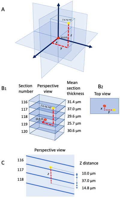
Schematic diagrams illustrating the principle used to determine the three‐dimensional coordinates of each large interneuron in the sections from the dorsal striatum (CPu). (A) Diagram illustrating the x, y, z coordinates of an example neuron (yellow asterisk) relative to the reference neuron (red asterisk). The reference neuron is near the center of the middle section of the five consecutive sections, and its location is defined as (0,0,0). (B1) Example of x, y, z coordinate determination for a neuron in Rat 3, Section 116. (B2) Top view, showing how the x and y coordinates of the example neuron were obtained from its position relative to the reference neuron in the collapsed 2D overlaid map. (C) Perspective view of (B1). The thickness of each section and the position of the neuron within the section were taken into account to determine the z coordinate. The z position of the neuron within Section 116 was measured from the lower surface of the section (10 µm) and added to the thickness of the intervening Section 117 (37 µm) plus the distance of the reference neuron from the upper surface of Section 118 (14.8 µm). For the neuron shown, this yielded a z position of 61.8 µm from the reference neuron. Anatomically, the sections indicated in (B1) are in the coronal plane, with Section 116 being the most anterior. Thus, the z dimension corresponds to the anterior–posterior axis of the brain.

To determine the z‐coordinate for each neuron, we used the following procedure. An Olympus BH2 microscope, using a ×2.5 eyepiece and a ×100 objective lens, and an attached microcator were used to measure the z‐distance within a section and the thickness of each section (Figure 8C). The z‐distance within a section for each identified neuron was obtained in µm from the known section thickness of the section it was in and its distance from the lower surface of the section (Figure 8C). The total z‐distance to the reference neuron could thus be determined (Figure 8C). The + or − sign at the front of each numbered neuron had to be carefully figured out because this is important information in locating the neuron at its exact place. Thus, every neuron had + or − with x, y, and z (Figure 8A,B1).

Totally, the x, y, z coordinates were determined for 805 large interneurons in the 5 consecutive sections of Rat 3 (Figure 7B,D) and for 897 large interneurons in the 5 consecutive sections for Rat 7 (Figure 7A,C). The collection of a 3D data set of 1000 points represents a considerable experimental effort (Reed and Howard 1997).

For each rat, the x, y, z values were collated into a computer spreadsheet for subsequent 3D spatial analyses [see next section].

4. Results

The CINs in the striatum are known to receive asymmetric synaptic input from glutamate projection neurons in the PFN of the thalamus (Consolo et al. 1996; Lapper and Bolam ¹⁹⁹²). Therefore, in the present study, we focused on these two neural populations. Our results were based on a total of 11 Sprague‐Dawley rats. We first measured the total volume of each PFN (N = 6) and the striatum (N = 5). We then measured absolute numbers of all (mostly glutamatergic) neurons in the PFN and immunostained CINs in the striatum. Finally, we analyzed the 3D spatial distribution of the large, mostly CINs in subregions of the striatum (N = 2, using sections from the same rats used for PFN analyses).

4.1. Estimation of the Total Volume of Each PFN and the Striatum

We used the Cavalieri method to measure the total volume of each PFN and striatum. The total number of points counted ranged from 130 to 198 for the PFN in six rats and from 98 to 115 for the striatum in five rats (∑P, see Tables 1 and 2). This complied with the guiding principle of counting 100–200 points per structure (Gundersen and Jensen 1987). Thus, very reliable estimates were obtained, with the CE (∑P) being much less than 0.10 (Gundersen and Jensen 1987) (see Table 3). The average section thickness for each rat was 31.9 µm for the PFN even though the sections were cut at 40 µm (Table 1) and 8.9 µm for the striatum when sections were cut at 20 µm (Table 2). Thus, it is necessary to measure the actual section thickness each time. CE values of section thickness for both the PFN and striatum were much less than 0.1 (data not shown), indicating that the sections were acceptably uniform and can be used in this study.

The resulting mean total volume estimates (V in Tables 1 and 2) were also acceptably accurate because the observed mean variance of the individual total volume for the PFN estimates [CE², e.g., (0.025)², see Table 3] was less than half the observed variance for the total volume estimates [CV², e.g., (0.119)², see Table 1] for six rats. For the striatum, the [CE², e.g., (0.031)², see Table 3] was also less than half the observed variance for the total volume estimates [CV², e.g., (0.103)², see Table 2] for five rats. This indicates that the major factor contributing to the overall variability was the true interanimal differences in total volume and not the precision of the estimates made with the stereological techniques employed (West and Gundersen 1990).

4.2. Estimation of the Numerical Density, or Nv, of the PFN Neurons and of the Striatal CINs

The sum of disector neurons counted (i.e., ∑Q ⁻) for each rat ranged from 291 to 388 in the PFN (see Table 1) and from 129 to 171 for each rat for the striatum. The disector neurons counted per rat for the PFN are greater than the number suggested as a guiding principle, that is, 100–200 particles or profiles per individual (Gundersen et al. 1988). When combined with the total number of frames sampled (∑F), the mean number of disector neurons sampled per disector volume (Q ⁻) was always greater than 1 but less than 2 (Tables 1 and 2). This complies with the guideline of sampling one to two neurons per disector volume (West and Gundersen 1990; West et al. ¹⁹⁹¹).

The average CE for the mean number of disector neurons per frame (∑Q ⁻/∑F) for the PFN and the striatum was less than 0.10 (see Table 3), indicating that reliable estimates were obtained. For the striatum, the observed mean variance of the individual Nv estimates [CE², e.g., (0.082)², see Table 3] was less than half the observed variance for the Nv for the group [CV², e.g., (0.231)², see Table 2]. This also indicates that the major factor contributing to the overall variability was the true interanimal differences in neuronal density and not the precision of the estimates made with the stereological techniques employed (West and Gundersen 1990).

However, for the PFN, the observed mean variance of the individual Nv estimates [CE², e.g., (0.059)², see Table 3] was not less than half the observed variance for the Nv for the group [CV², e.g., (0.034)², see Table 1]. This is because the interanimal variation in the Nv of 3.4% is much lower than the usual biological variation between animals of 10%–15% (Braendgaard et al. 1990). If, for example, the CV² had been (0.10)², then the CE² of (0.059)² would have been less than half. With this in mind, and in consideration of a CE (∑Q ⁻/∑F) of much less than 0.1 for all six rats (see Table 1), the Nv estimates are probably acceptably accurate.

4.3. Total Neuronal Number (N) of Thalamic Parafascicular and Striatal Cholinergic Neurons

It can be seen from Table 3 that the average CE values for the total number of PFN neurons of six rats [i.e., CE(N)] was 0.060, and 0.082 for the striatum of five rats. This indicates that reliable estimates (CE ≤ 0.10) were probably obtained. For all six parafascicular nuclei, the observed mean variance of the individual total neuronal number estimates [CE², e.g., (0.060)², see Table 3] was less than half the observed mean relative variance of the group [CV², e.g., (0.107)², see Table 1). For all five striata, the observed mean variance of the individual total neuronal number estimates [CE², e.g., (0.082)², see Table 3] was less than half the observed mean relative variance of the group [CV², e.g., (0.14)², see Table 2). These analyses suggest that the major factor contributing to the overall variability was the true interanimal differences in total neuronal numbers and not the precision of the estimates made with the stereological techniques employed (Oorschot 1996; West and Gundersen ¹⁹⁹⁰).

It was found that the right PFN consisted of 30,073 ± 3216 (mean ± SD) neurons (see Table 1). It was also found that the right striatum consisted of 10,778 ± 1513 (mean ± SD) CINs (see Table 2).

4.4. 3D Spatial Analyses

Anterior serial sections (Rat 7) and posterior serial sections (Rat 3) were used in the 3D spatial analysis. The posterior serial sections contained a total number of n = 805 CINs in a volume of 1.20 × 10⁹ µm³, thus having a mean density of 6.71 × 10⁻⁷ µm⁻³. The anterior serial sections contained n = 897 CINs in a volume of 1.30 × 10⁹ µm³, thus having a mean density of 7.03 × 10⁻⁷ µm⁻³.

Previous work has reported clustering of CINs in the rat striatum (Matamales et al. 2016), and inspection of the map in Figure 7A,B also suggested clustering. In an initial exploratory analysis, we tested for clustering using the standard form of Ripley's K‐function, and this also indicated clustering (not shown). However, this analysis is based on a comparison with a homogeneous spatial Poisson distribution (i.e., a completely spatially random distribution) over an observation region equal in size and shape to each sample. Because of this assumption of homogeneity, the standard form of Ripley's K‐function can give a false positive result suggesting clustering when the density is inhomogeneous.

Previous work has indicated gradients in the density of CINs (Bernacer et al. 2007; Matamales et al. ²⁰¹⁶) and their neurochemical markers (Hortnagl et al. 2020). If density gradients exist, then the distribution of CINs in the striatum may not be homogeneous. Examination of the probability density determined from the 3D distribution is shown as a contour plot of probability density in Figure 9A,B. On inspection, this figure appears to show considerable variation in density in both data sets. For example, there are regions of very low density and other regions of higher density. If the observed distribution is significantly different from a homogeneous spatial Poisson distribution, that is, if the observed distribution is not consistent with a homogeneous spatial Poisson distribution, the standard K‐function analysis is invalid and the inhomogeneous K‐function should be used.

FIGURE 9.

Inhomogeneity of the density of large interneurons in the sections from the dorsal striatum (CPu). (A and B) Probability density function contour plots across anterior (A, Rat 7) and posterior (B, Rat 3) regions of the rat striatum. Each plot displays a collapsed 2D density distribution of the neuronal somata identified in anterior and posterior regions. Notice the seeming inhomogeneity in the density distribution of the plots. White dotted lines delineate boundaries of the anterior and posterior regions of the striatum. (C–F) Statistical analysis of the 3D spatial distribution of CINs reveals the density distribution is inhomogeneous. The sampling method involved identification of cells in predefined regions (red and blue cells). The density of cells in each red and blue region was compared. See text for explanation. (C and D) Medial vs. lateral comparison for anterior (C) and posterior (D) sections. (E and F) Dorsal vs. ventral comparison for anterior (E) and posterior (F) sections. In (C)–(F), coordinates shown on mediolateral (lower side) and dorsoventral (right side) axes are in µm relative to the central origin.

We first tested the null hypothesis that the observed locations of CINs were drawn from a homogeneous spatial Poisson distribution over an observation region equal in size and shape to each sample (Illian et al. 2008). We found for anterior serial sections, χ ² = 76.06, p = 7.123 × 10⁻⁸, and for posterior serial sections, χ ² = 50.8, p = 0.00072, using the SpatialRandomnessTest (Mathematica 13.0). Thus, the null hypothesis was not supported by the data in either case. The χ ² statistic, however, does not distinguish between inhomogeneity and clustering. A significant difference from a homogeneous spatial Poisson distribution could be due to clustering in a homogeneous distribution or due to inhomogeneity. It is also possible for a distribution to be both inhomogeneous and clustered (Illian et al. 2008). Therefore, we tested separately for inhomogeneity and clustering.

4.4.1. Testing for Inhomogeneity

To test for inhomogeneity, we created dorsal, ventral, lateral, and medial subregions and tested whether the point densities were equal (Illian et al. 2008). The regions were sampled as shown in Figure 9C–F. Using this approach for anterior serial sections, we found F _213,135 = 1.58, p = 0.002 (dorsal vs. ventral) and F _285,215 = 1.33, p = 0.015 (medial vs. lateral). In posterior serial sections, we found F _115,227 = 1.97, p = 0.000 (dorsal vs. ventral) and F _277,187 = 1.48, p = 0.002 (medial vs. lateral). Thus, there was evidence of inhomogeneity in both rats in both the anterior and posterior sections, in both the dorsoventral and mediolateral comparisons.

4.4.2. Testing for Clustering in an Inhomogeneous Distribution

To test for clustering, we first measured nearest neighbor distributions in 3D for the same set of serial sections used to generate Figure 9A,B, and compared these with simulated inhomogeneous Poisson distributions based on the spatial density distribution of neurons. These showed that the observed mean nearest neighbor distances were not significantly different from the simulated inhomogeneous Poisson distributions (Figure 10A,B). However, the mean nearest neighbor distance in the sample could arise from a mixture of clustering and regularity. Thus, we also analyzed the spatial distribution using the inhomogeneous K‐function (Baddeley et al. 2001; Marcon and Puech ²⁰⁰⁹), which is able to reveal clustering on different spatial scales. Analysis of inhomogeneous K‐functions (Figure 10C,D) and their corresponding L‐functions (Figure 10E,F) showed no difference between the observed distribution and simulated (Baddeley et al. 2014) inhomogeneous Poisson distributions.

FIGURE 10.

Statistical tests of clustering of large interneurons. (A and B) Nearest neighbor probability density functions of large interneurons in the anterior (A) and posterior (B) regions of the striatum, using the same set of serial sections used to generate Figures 9A,B. The histogram shows the distribution of the mean nearest neighbor distances measured in each instance of an ensemble of n = 10,000 simulations, and the dotted black line indicates the mean value of the experimentally measured distributions. The fitted normal distribution with the mean (μ) and standard deviation (σ) is shown on each histogram (orange line). The mean nearest neighbor distances in the observed distributions were not significantly different from the simulated distributions in the anterior and posterior regions examined. Probability values were calculated using the method described by Baddeley et al. (2014). For a two‐tailed test, the probability is calculated from the number of simulated values (k) that are larger than the observed value (if the observed value is greater than the mean of the simulated values) or smaller than the observed value (if the observed value is smaller than the mean of the simulated values) and the total number of simulated values (n), using the formula p = 2k/(n + 1). For the anterior section, k = 4425, and for the posterior section, k = 261. (C and D) Inhomogeneous K‐functions for the anterior (C) and posterior (D) regions were calculated using the method of Baddeley et al. (2001) and the Ripley K‐function generalized to inhomogeneous populations: ${\widehat{K}}_{\mathrm{In}hom}(t)=\frac{1}{|W|}{\sum }_{y_i\in Y\cap W}{\sum }_{y_j\in Y\cap W}\frac{{\omega }_{y_i,y_j}I(\parallel y_i-y_j\parallel \le t)}{\lambda (y_i)\lambda (y_j)},0\le t\le t^{\ast }$ where $\lambda (y_i)$ ₎ and $\lambda (y_j)$ are the local densities of the points $y_i$ and $y_j$, ${\omega }_{y_i,y_j}$ is the edge correction factor (Ripley 1977), Y is the inhomogeneous point distribution, W is the volume within radius t, and ||y_i  − y_j || ≤ t is the indicator functiowhich is 1 if the distance from point (i) to point (j) is less than or equal to radius t. Blue lines represent 10,000 simulations of inhomogeneous neuronal arrangements in the anterior and posterior regions of the striatum. Black dotted lines illustrate the observed distribution. (E and F) Closer examination of spatial distribution using L‐functions based on the formula: $L(t)=\sqrt[3]{[{\widehat{K}}_{\mathrm{Inhom}}(t)-\mu ({\widehat{K}}_{\mathrm{Inhom}}(t))]}$ where μ is the mean function. As all observed values fell within the simulation envelope, we can conclude there is no significant clustering in either anterior or posterior regions.

4.5. Cross‐Check of the Total Number of Large, Mostly Cholinergic Striatal Interneurons

The total number of large, mostly CINs within the rat striatum was doubly checked in this study based on the data obtained from the five sections of each of Rats 3 and 7 (Table 4). It was known that there are 805 and 897 large interneurons within five sections in each of Rats 3 and 7 (Table 4), respectively. The striatal subvolume that these interneurons occupy can be obtained by multiplying the average area of the five sections by the summated section thickness of the five sections. Because the total volume of the striatum for Rats 3 and 7 is known from the study of Oorschot (1996), the total number of these larger interneurons within the rat striatum could be obtained. It was shown that there are 14,296 ± 2200 (mean ± SD) large interneurons (Table 4).

TABLE 4.

Total number of large, mostly cholinergic interneurons estimated for Rats 3 and 7.

	Rat 3	Rat 7
Section numbers	116–120	101–105
Area for five sections	7.75 mm2	8 mm2
Neurons in five sections	805	897
Volume of five sections	1.196 mm3	1.275 mm3
Volume of striatum a	23.55 mm3	18.11 mm3
Total number of neurons	15,852	12,741
Mean	14,296
SD	2200
CV	0.15

Note: The raw data for each section thickness for Rat 3 are Section 116—31.4 µm, Section 117—37 µm, Section 118—29.6 µm, Section 119—25.7 µm, and Section 120—30.6 µm. For Rat 7, the raw data for each section thickness are Section 101—31.68 µm, Section 102—31.97 µm, Section 103—31.75 µm, Section 104—30.26 µm, and Section 105—33.73 µm.

^a Data from Oorschot (1996) study.

4.6. Summary of Findings

Figure 11 illustrates the relationship between the structures studied and provides a summary of the numerical findings.

FIGURE 11.

Schematic diagram of a sagittal section through the rat brain illustrating the relationship between the structures studied. A summary of the new numerical findings from this study is included. CPu, caudate‐putamen; PFN, parafascicular nucleus; “*,” spiny projection neuron. Source: Diagram modified from Paxinos G. (1995). The Rat Nervous System, with copyright approval obtained.

5. Discussion

The absolute numbers of thalamic PFN neurons and striatal CINs in young adult Sprague‐Dawley rats were estimated using unbiased stereological methods. On average, the right PFN contained 30,073 neurons, and the right striatum contained 10,778 CINs. Analysis of the 3D spatial distribution of the large, mostly CINs revealed that they were randomly positioned with no evidence of clustering. As far as we are aware, this is the first time that such data have been obtained. This new knowledge is relevant to information processing operations of these neurons and their role in cognitive operations such as behavioral flexibility.

5.1. Absolute Number of Rat Striatal CINs

The number of CINs in the rat striatum has been reported previously, yet the studies have some methodological caveats. In the normal Wistar rat, Larrson et al. (2001) reported the “total number” of ChAT neurons in the caudate‐putamen as 6800 unilaterally. However, they did not include the rostral part of the caudate‐putamen in their measurement, and this seems likely to have contributed to the lower unilateral total number reported when compared to the current study. In the normal Lewis rat, a total number of 6790 CINs in the striatum (presumably the caudate‐putamen) is reported (Champy et al. 2004). However, it is unclear if this is a unilateral or bilateral total number and whether the entire rostrocaudal extent of the striatum was analyzed. The latter context and the different subspecies of rat may have contributed to the lower total number of striatal CINs reported by Champy et al. (2004) in comparison to the current study.

Van Vulpen and van der Kooy (1996) estimated the total number of ChAT‐positive neurons within the head of the rat striatum using the method of Abercrombie (1946) that takes into account the size of the cells being counted. They observed a total number of 5500 ChAT‐positive neurons within the head of the striatum at postnatal Day 17 (see their Figure 5). The head of the striatum was defined as the entire striatum rostral to the external globus pallidus and dorsal to the nucleus accumbens (van Vulpen and van der Kooy ¹⁹⁹⁶). On the basis of this definition, the percentage of the striatum that the head occupies can be determined from the raw data of Oorschot (1996) for the Cavalieri estimate of total striatal volume. The head of the striatum was found to occupy 59% of the total striatal volume on average. By extrapolation of the data from van Vulpen and van der Kooy (1996), the total number of ChAT‐positive neurons within the entire striatum would then be 9300. This is similar to the total number observed at postnatal Day 19 in the striatum in the present study. These similar numbers from different laboratories suggest that the total numbers obtained are close to reality and also suggest that the Abercrombie method and the physical disector method are equally valid methods for estimating the total number of rat striatal CINs (see also van Vulpen and van der Kooy ¹⁹⁹⁹).

In the current study, the total number of 14,300 histochemically detected large, mostly CINs is higher than the total number of immunocytochemically detected CINs. The histochemically stained neurons might have included some of the large GABAergic/parvalbumin interneurons (Kita et al. 1990). Using Chang et al.’s (1982) criterion of a large neuron (a cross‐sectional area of >300 µm²), examination of Figure 5 of Kita et al. (1990) indicates that 20% of their GABAergic/parvalbumin neurons meet this criterion. Given a total number of 16,900 GABAergic/parvalbumin neurons in the unilateral striatum (Luk and Sadikot, 2001), the total number of large striatal GABAergic/parvalbumin neurons could be 3380 (i.e., 16,900 × 0.20), which is similar to the total number of non‐ChAT large interneurons estimated from the current data (14,300 − 10,778 = 3522). These data suggest that the total number results in this article are close to reality for the respective neuronal populations.

In this study, the physical/optical disector method (for Nv) and the Cavalieri method (for Vref) were used to obtain the absolute number of CINs and PFN neurons (i.e., Nv × Vref) instead of the physical/optical fractionator method (Slomianka 2021; West et al. ¹⁹⁹¹). In the physical/optical fractionator method, neuronal number is measured in a known fraction of the entire structure of interest (e.g., the PFN or the striatum), and then this number is multiplied by the inverse of the fraction to obtain the absolute number of neurons (see Slomianka (2021) for further details). Both the Nv × Vref and the physical/optical fractionator methods are valid approaches for estimating the absolute number of neurons, as long as specific procedures are undertaken. The physical disector and Cavalieri method were used to estimate the absolute number of striatal CINs in frozen sections in this study. This does not create a problem with shrinkage in frozen sections, even though they shrink considerably in height, since the disector counts and Cavalieri counts were done on the same sections at the same stage of processing. The same sections at the same stage of processing were also analyzed for the absolute number of PFN neurons, using glycol methacrylate sections. The Nv × Vref approach has considerations for data homogeneity, as the mean of all disector probe sites is used for the final calculation, leading to potential skewing of the data if too many sites with no counts (i.e., neurons) are encountered. The size of the unbiased sampling frame can be increased to overcome this in pilot studies, which was completed in this study. The Nv × Vref method also relies on a separate estimate of the total reference volume, which could yield an additional potential source of variation depending on the precision of this estimate. The precision of our estimates had a CE of <3.4% for each individual, which is highly acceptable. For the physical/optical fractionator approach, a precise definition of the edges of a structure is not needed, yet one does need to know if one is sampling in the structure of interest or not. This is based on its internal anatomy relative to adjacent structures.

5.2. Relative Numbers of PFN Neurons and CINs

The ratio of the total number of PFN neurons to the total number of CINs in the rat was found to be approximately 3:1 in the current study. In humans, however, a ratio of 1:1 can be inferred from the similar numbers of PFN neurons (657,000 ± 37,000) reported by Henderson et al. (2000) and large‐sized, presumably CINs in human males (670,000) and females (570,000) (Lange et al. 1976; Schroder et al. ¹⁹⁷⁵).

5.3. Relative Numbers of SPNs Versus CINs and PFN Neurons

When compared to the total number of 2.79 million striatal SPNs unilaterally in the Sprague‐Dawley rat (Oorschot 1996), the CINs constitute less than 0.4% of the total striatal neuronal population. This is a similar percentage to that reported for the mouse striatum (Peterson et al. 1999), yet it differs from an earlier rat study that reported a proportion of 1.7% (Phelps et al. 1985). There are several possible reasons for the difference among these estimates. Peterson et al. (1999) immunostained CINs and estimated their total number using the optical fractionator method. It was found that there were, on average, 5000 CINs in the mouse striatum unilaterally compared to a total number of 1.69 million striatal neurons on average (Peterson et al. 1999), indicating that less than 0.3% of the neurons in the mouse striatum are CINs. In contrast, the immunocytochemical study by Phelps et al. (1985) was based on counting 162 ChAT‐immuno‐positive neurons among the 8950 neurons that were mapped and counted in a subsection of the striatum (i.e., anterior and posterior coronal vibratome sections). Thus, the method used to estimate the number or percentage of ChAT neurons was not based on an analysis of the entire (i.e., complete) striatum. Taken together, the 3D stereological data suggest that less than 0.4% of striatal neurons might be close to reality for CINs in the rat and mouse striata.

In addition to innervating the CINs, the PFN neurons also form asymmetrical, presumably excitatory, synapses with the SPNs (Lapper and Bolam 1992). The total number of PFN neurons reported in the present study and the total number of striatal SPNs (of 2.79 million), unilaterally, in the Sprague‐Dawley rat (Oorschot 1996), suggest a ratio of 93:1 SPNs to PFN neurons. A larger ratio (152:1) occurs in humans based on a total number of 100 million striatal neurons (Lange et al. 1976) and 657,000 PFN neurons (Henderson et al. (2000). The high degree of divergence of PFN neurons to SPNs in both rats and humans may allow a widespread influence of PFN activity in the CPu.

The differences in the ratios of PFN neurons to CINs and SPNs may reflect important species differences that are significant in evolutionary terms and await further comparative research in other species. It needs to be recognized, however, that this important total neuronal number data is a first step in understanding information processing. Other data are now needed before firm conclusions can be made. The data now needed includes the total number of synaptic connections made by an afferent neuron, how many different neurons are innervated by each neuron, the spatial extent and local configuration of an axonal arborization, physiological considerations about how information is encoded in spike trains, and the number of converging afferents that are required to generate a decisive effect on a postsynaptic neuron.

5.4. 3D Spatial Distribution of Striatal CINs

Whether CINs of the striatum are clustered or not has been investigated in 2D analyses over many years. We used a unique 3D mapping approach combined with 3D spatial statistical analysis to address this question in the rat. The locations of presumed CINs in anterior and posterior sections of the striatum were mapped in 3D coordinates. Our analysis showed that the spatial density distribution of CINs is non‐uniform, with gradients in the density in both the dorsoventral and mediolateral directions of anterior and posterior sections. We then tested for clustering using an approach that took into account the inhomogeneous spatial density distribution of the observed samples. When the inhomogeneous density of the observed distribution is correctly taken into account, comparison of the observed spatial distribution with computer‐generated random distributions revealed no evidence of clustering.

Previous studies have reported conflicting qualitative observations concerning whether CINs were clustered. For example, Mufson et al. (1989) reported that in the human caudate and putamen, CINs did not appear evenly distributed but in many instances occurred in small clusters. In contrast, Graybiel et al. (1986) observed that in monkey and cat striatum, ChAT‐positive cell bodies were not obviously clustered.

Even when quantitative methods have been used, conflicting results concerning clustering have been reported. Matamales et al. (2016) performed a 2D analysis of clustering in the rat striatum, section by section in the coronal plane. Using Ripley's K‐function to determine the presence or absence of clustering in individual 2D sections, they found that 31 out of 76 sections (40%) exhibited significant differences from simulated distributions based on an assumption of homogeneous density. Matamales et al. (2016) also speculated that a 3D analysis of the whole striatum would find a higher degree of clustering. However, Matamales et al. (2016) also reported that the 2D density of CINs was inhomogeneous on a local scale of 200 µm, which violated the assumption of homogeneous density that is made in Ripley's K‐function. Because the appearance of clustering can arise from inhomogeneity, it is probable that the incidence of clustering was overestimated by this method.

Using an adaptation of Ripley's K‐function suitable for inhomogeneous spatial distributions (Baddeley et al. 2001; Christensen and Møller ²⁰²⁰; Marcon and Puech ²⁰⁰⁹), we found no evidence for clustering in the 3D spatial distribution of CINs in anterior and posterior regions of the rat striatum, each analyzed through five consecutive serial sections across the entire striatum in the coronal plane. We first determined that the 3D spatial distribution of the CINs was not completely spatially random and that there were significant differences in the density of CINs between volumes within each subregion. We then estimated the 3D spatial density of the distributions and used these estimates to generate an envelope of inhomogeneous 3D Poisson distributions for each region with which to compare the observed distributions. This comparison revealed no significant departures from complete spatial randomness after the inhomogeneity of density was taken into account. Thus, we found no evidence for spatial clustering of CINs in the striatal areas we examined.

Our observation of differences in density of CINs from medial to lateral is consistent with previous reports in the rat (Matamales et al. 2016), mouse (Gangarossa et al. 2013), and human striatum (Bernacer et al. 2007; Hortnagl et al. ²⁰²⁰). The density of SPNs also shows regional variation like the CINs in the present study but along the rostro‐caudal axis. When this was taken into account in the analysis, their spatial distribution was also found not to be clustered (Gangarossa et al. 2013).

It needs to be acknowledged that the rare 3D spatial analyses undertaken within the current study, across two rats, did not cover the entire striatum. Thus, the spatial distribution could be considered as primarily a projection rather than a 3D distribution, because the slice thickness (µm in z‐direction) compared to the area (mm in x‐ and y‐direction) of the structures in the section is very small. The analyses were also not undertaken on neurons that were immunohistochemically stained for ChAT. These approaches have been recently completed for the entire mouse striatum (Carrasco et al. 2022). The same approaches now need to be undertaken in the rat to extend the current results.

6. Conclusions: The PFN and the Striatal CINs

On the basis of the absolute number data of the current study, the relatively high ratio of PFN neurons to CINs raises the possibility of specific control of CINs by PFN neurons. We found no evidence of spatial clustering of CINs in the striatal areas we examined. Biologically, if the spatial arrangement of neurons does reflect the functional operations performed by the CINs circuitry, how does this anatomy subserve function? One possibility is that randomness may be the best structure for some functions. For example, random spatial distribution of somata is a simple way of giving equal probability to all neighborhood relationships, which can provide an unbiased starting point for the growth of axons and dendrites to establish network connectivity.

Author Contributions

Rong Zhang: data acquisition, analysis. Jeffery R. Wickens: analysis, interpretation, editing, software tools. Andres Carrasco: analysis, interpretation, editing, software tools. Dorothy E. Oorschot: conception and design, analysis, interpretation, drafting, editing.

Ethics Statement

All experiments were carried out in accordance with the regulations of the University of Otago Committee on Ethics in the Care and Use of Laboratory Animals.

Conflicts of Interest

The authors declare no conflicts of interest.

Peer Review

The peer review history for this article is available at https://publons.com/publon/10.1002/cne.70050.

Data Availability Statement

The 3D x, y, z coordinates of the location of large striatal interneurons in the rat are available at the following public repository: FIGSHARE repository.

References

- Abercrombie, M. 1946. “Estimation of Nuclear Population From Microtome Sections.” Anatomical Record 94: 239–247. [DOI] [PubMed] [Google Scholar]
- Aoki, S. , Liu A. W., Zucca A., Zucca S., and Wickens J. R.. 2015. “Role of Striatal Cholinergic Interneurons in Set‐Shifting in the Rat.” Journal of Neuroscience 35, no. 25: 9424–9431. [DOI] [PMC free article] [PubMed] [Google Scholar]
- Aoki, S. , Liu A. W., Zucca A., Zucca S., and Wickens J. R.. 2017. “New Variations for Strategy Set‐Shifting in the Rat.” JOVE 119: e55005. [DOI] [PMC free article] [PubMed] [Google Scholar]
- Aosaki, T. , Graybiel A. M., and Kimura M.. 1994. “Effect of the Nigrostriatal Dopamine System on Acquired Neural Responses in the Striatum of Behaving Monkeys.” Science 265: 412–415. [DOI] [PubMed] [Google Scholar]
- Apicella, P. 2007. “Leading Tonically Active Neurons of the Striatum From Reward Detection to Context Recognition.” Trends in Neuroscience (Tins) 30, no. 6: 299–306. [DOI] [PubMed] [Google Scholar]
- Armstrong, D. M. , Saper C. B., Levey A. I., Wainer B. H., and Terry R. D.. 1983. “Distribution of Cholinergic Neurons in Rat Brain: Demonstrated by the Immunocytochemical Localization of Choline Acetyltransferase.” Journal of Comparative Neurology 216, no. 1: 53–68. [DOI] [PubMed] [Google Scholar]
- Baddeley, A. J. , Diggle P. J., Hardegen A., Lawrence T., Milne R. K., and Nair G.. 2014. “On Tests of Spatial Pattern Based on Simulation Envelopes.” Ecological Monographs 84, no. 3: 477–489. [Google Scholar]
- Baddeley, A. J. , Moller J., and Waagepetersen R.. 2001. “Non‐ and Semi‐Parametric Estimation of Interaction in Inhomogeneous Point Patterns.” Statistica Neerlandica 54, no. 3: 329–350. [Google Scholar]
- Baldi, G. , Russi G., Nannini L., Vezzani A., and Consolo S.. 1995. “Trans‐Synaptic Modulation of Striatal Ach Release In Vivo by the Parafascicular Thalamic Nucleus.” European Journal of Neuroscience 7, no. 5: 1117–1120. [DOI] [PubMed] [Google Scholar]
- Bernacer, J. , Prensa L., and Gimenez‐Amaya J. M.. 2007. “Cholinergic Interneurons Are Differentially Distributed in the Human Striatum.” PLoS ONE 2, no. 11: e1174. [DOI] [PMC free article] [PubMed] [Google Scholar]
- Bjugn, R. , and Gundersen H. J.. 1993. “Estimate of the Total Number of Neurons and Glial and Endothelial Cells in the Rat Spinal Cord by Means of the Optical Disector.” Journal of Comparative Neurology 328, no. 3: 406–414. [DOI] [PubMed] [Google Scholar]
- Bolam, J. P. , Wainer B. H., and Smith A. D.. 1984. “Characterization of Cholinergic Neurons in the Rat Neostriatum. A Combination of Choline Acetyltransferase Immunocytochemistry, Golgi‐Impregnation and Electron Microscopy.” Neuroscience 12, no. 3: 711–718. [DOI] [PubMed] [Google Scholar]
- Bradfield, L. A. , Bertran‐Gonzalez J., Chieng B., and Balleine B. W.. 2013. “The Thalamostriatal Pathway and Cholinergic Control of Goal‐Directed Action: Interlacing New With Existing Learning in the Striatum.” Neuron 79, no. 1: 153–166. [DOI] [PMC free article] [PubMed] [Google Scholar]
- Braendgaard, H. , Evans S. M., Howard C. V., and Gundersen H. J.. 1990. “The Total Number of Neurons in the Human Neocortex Unbiasedly Estimated Using Optical Disectors.” Journal of Microscopy 157, no. Pt 3: 285–304. [DOI] [PubMed] [Google Scholar]
- Brown, H. D. , Baker P. M., and Ragozzino M. E.. 2010. “The Parafascicular Thalamic Nucleus Concomitantly Influences Behavioral Flexibility and Dorsomedial Striatal Acetylcholine Output in Rats.” Journal of Neuroscience 30, no. 43: 14390–14398. [DOI] [PMC free article] [PubMed] [Google Scholar]
- Cachope, R. , Mateo Y., Mathur B. N., et al. 2012. “Selective Activation of Cholinergic Interneurons Enhances Accumbal Phasic Dopamine Release: Setting the Tone for Reward Processing.” Cell Reports 2, no. 1: 33–41. [DOI] [PMC free article] [PubMed] [Google Scholar]
- Carrasco, A. , Oorschot D. E., Barzaghi P., and Wickens J. R.. 2022. “Three‐Dimensional Spatial Analyses of Cholinergic Neuronal Distributions Across the Mouse Septum, Nucleus Basalis, Globus Pallidus, Nucleus Accumbens, and Caudate‐Putamen.” Neuroinformatics 20, no. 4: 1121–1136. [DOI] [PMC free article] [PubMed] [Google Scholar]
- Champy, P. , Hoglinger G. U., Feger J., et al. 2004. “Annonacin, a Lipophilic Inhibitor of Mitochondrial Complex I, Induces Nigral and Striatal Neurodegeneration in Rats: Possible Relevance for Atypical Parkinsonism in Guadeloupe.” Journal of Neurochemistry 88, no. 1: 63–69. [DOI] [PubMed] [Google Scholar]
- Chang, H. T. , Wilson C. J., and Kitai S. T.. 1982. “A Golgi Study of Rat Neostriatal Neurons: Light Microscopic Analysis.” Journal of Comparative Neurology 208: 107–126. [DOI] [PubMed] [Google Scholar]
- Christensen, H. S. , and Møller J.. 2020. “Modelling Spine Locations on Dendrite Trees Using Inhomogeneous Cox Point Processes.” Spatial Statistics 39: 100478. [Google Scholar]
- Consolo, S. , Baldi G., Giorgi S., and Nannini L.. 1996. “The Cerebral Cortex and Parafascicular Thalamic Nucleus Facilitate In Vivo Acetylcholine Release in the Rat Striatum Through Distinct Glutamate Receptor Subtypes.” European Journal of Neuroscience 8, no. 12: 2702–2710. [DOI] [PubMed] [Google Scholar]
- DiFiglia, M. 1987. “Synaptic Organization of Cholinergic Neurons in the Monkey Neostriatum.” Journal of Comparative Neurology 255, no. 2: 245–258. [DOI] [PubMed] [Google Scholar]
- Dimova, R. , Vuillet J., Nieoullon A., and Kerkerian‐Le Goff L.. 1993. “Ultrastructural Features of the Choline Acetyltransferase‐Containing Neurons and Relationships With Nigral Dopaminergic and Cortical Afferent Pathways in the Rat Striatum.” Neuroscience 53, no. 4: 1059–1071. [DOI] [PubMed] [Google Scholar]
- Ding, J. B. , Guzman J. N., Peterson J. D., Goldberg J. A., and Surmeier D. J.. 2010. “Thalamic Gating of Corticostriatal Signaling by Cholinergic Interneurons.” Neuron 67, no. 2: 294–307. [DOI] [PMC free article] [PubMed] [Google Scholar]
- Doig, N. M. , Magill P. J., Apicella P., Bolam J. P., and Sharott A.. 2014. “Cortical and Thalamic Excitation Mediate the Multiphasic Responses of Striatal Cholinergic Interneurons to Motivationally Salient Stimuli.” Journal of Neuroscience 34, no. 8: 3101–3117. [DOI] [PMC free article] [PubMed] [Google Scholar]
- Fonnum, F. , and Walaas S. I.. 1979. “Localization of Neurotransmitter Candidates in Neostriatum.” In The Neostriatum, 53–69. Pergamon Press. [Google Scholar]
- Galvin, K. A. , and Oorschot D. E.. 2003. “Continuous Low‐Dose Treatment With Brain‐Derived Neurotrophic Factor or Neurotrophin‐3 Protects Striatal Medium Spiny Neurons From Mild Neonatal Hypoxia/Ischemia: A Stereological Study.” Neuroscience 118, no. 4: 1023–1032. [DOI] [PubMed] [Google Scholar]
- Gangarossa, G. , Espallergues J., Mailly P., et al. 2013. “Spatial Distribution of D1R‐ and D2R‐Expressing Medium‐Sized Spiny Neurons Differs Along the Rostro‐Caudal Axis of the Mouse Dorsal Striatum.” Front Neural Circuits 7: 124. [DOI] [PMC free article] [PubMed] [Google Scholar]
- Gleeson, P. , Steuber V., and Silver R. A.. 2007. “Neuroconstruct: A Tool for Modeling Networks of Neurons in 3D Space.” Neuron 54, no. 2: 219–235. [DOI] [PMC free article] [PubMed] [Google Scholar]
- Graybiel, A. M. , Baughman R. W., and Eckenstein F.. 1986. “Cholinergic Neuropil of the Striatum Observes Striosomal Boundaries.” Nature 323, no. 6089: 625–627. [DOI] [PubMed] [Google Scholar]
- Grillner, S. , and Robertson B.. 2016. “The Basal Ganglia Over 500 Million Years.” Current Biology 26, no. 20: R1088–R1100. [DOI] [PubMed] [Google Scholar]
- Groenewegen, H. J. , and Berendse H. W.. 1994. “The Specificity of the ‘Nonspecific’ Midline and Intralaminar Thalamic Nuclei.” Trends in Neuroscience (Tins) 17, no. 2: 52–57. [DOI] [PubMed] [Google Scholar]
- Gundersen, H. J. G. 1977. “Notes on the Estimation of the Numerical Density of Arbitrary Profiles: The Edge Effect.” Journal Microscopy‐Oxford 111: 219–223. [Google Scholar]
- Gundersen, H. J. G. 1986. “Stereology of Arbitrary Particles. A Review of Unbiased Number and Size Estimators and the Presentation of some New Ones, in Memory of William R. Thompson.” Journal of Microscopy 143, no. Pt 1: 3–45. [PubMed] [Google Scholar]
- Gundersen, H. J. G. , Bendtsen T. F., Korbo L., et al. 1988. “Some New, Simple and Efficient Stereological Methods and Their Use in Pathological Research and Diagnosis.” Acta Pathologica et Microbiologica Scandinavica 96: 379–394. [DOI] [PubMed] [Google Scholar]
- Gundersen, H. J. G. , and Jensen E.. 1987. “The Efficiency of Systematic Sampling in Stereology and Its Prediction.” Journal of Microscopy 147: 229–263. [DOI] [PubMed] [Google Scholar]
- Gundersen, H. J. G. , Jensen E. B. V., Kieu K., and Nielsen J.. 1999. “The Efficiency of Systematic Sampling in Stereology—Reconsidered.” Journal Microscopy‐Oxford 193: 199–211. [DOI] [PubMed] [Google Scholar]
- Henderson, J. M. , Carpenter K., Cartwright H., and Halliday G. M.. 2000. “Loss of Thalamic Intralaminar Nuclei in Progressive Supranuclear Palsy and Parkinson's Disease: Clinical and Therapeutic Implications.” Brain 123, no. Pt 7: 1410–1421. [DOI] [PubMed] [Google Scholar]
- Hortnagl, H. , Pifl C., Hortnagl E., Reiner A., and Sperk G.. 2020. “Distinct Gradients of Various Neurotransmitter Markers in Caudate Nucleus and Putamen of the Human Brain.” Journal of Neurochemistry 152, no. 6: 650–662. [DOI] [PMC free article] [PubMed] [Google Scholar]
- Illian, J. , Penttinen A., Stoyan H., and Stoyan D.. 2008. “The Homogeneous Poisson Point Process.” In Spatial Statistics and Modelling of Spatial Point Patterns, 57–97. Wiley. [Google Scholar]
- Izzo, P. N. , and Bolam J. P.. 1988. “Cholinergic Synaptic Input to Different Parts of Spiny Striatonigral Neurons in the Rat.” Journal of Comparative Neurology 269: 219–234. [DOI] [PubMed] [Google Scholar]
- Jones, E. G. 1985. The Intralaminar Nuclei. Jones E. G., The Thalamus. pp. 615–645. New York: Plenum Press. [Google Scholar]
- Kemp, J. M. , and Powell T. P.. 1971. “The Synaptic Organization of the Caudate Nucleus.” Philosophical Transactions of the Royal Society of London. Series B: Biological Sciences 262, no. 845: 403–412. [DOI] [PubMed] [Google Scholar]
- Kimura, M. , Minamimoto T., Matsumoto N., and Hori Y.. 2004. “Monitoring and Switching of Cortico‐Basal Ganglia Loop Functions by the Thalamo‐Striatal System.” Neuroscience Research 48, no. 4: 355–360. [DOI] [PubMed] [Google Scholar]
- Kita, H. , Kosaka T., and Heizmann C. W.. 1990. “Parvalbumin‐Immunoreactive Neurons in the Rat Neostriatum: A Light and Electron Microscopic Study.” Brain Research 536: 1–15. [DOI] [PubMed] [Google Scholar]
- Kubota, Y. , Inagaki S., Shimada S., Kito S., Eckenstein F., and Tohyama M.. 1987. “Neostriatal Cholinergic Neurons Receive Direct Synaptic Inputs From Dopaminergic Axons.” Brain Research 413: 179–184. [DOI] [PubMed] [Google Scholar]
- Lange, H. , Thorner G., Hopf A., and Schroder K. F.. 1976. “Morphometric Studies of the Neuropathological Changes in Choreatic Diseases.” Journal of the Neurological Sciences 28, no. 4: 401–425. [DOI] [PubMed] [Google Scholar]
- Lapper, S. R. , and Bolam J. P.. 1992. “Input From the Frontal Cortex and the Parafascicular Nucleus to Cholinergic Interneurons in the Dorsal Striatum of the Rat.” Neuroscience 51, no. 3: 533–545. [DOI] [PubMed] [Google Scholar]
- Larsson, E. , Lindvall O., and Kokaia Z.. 2001. “Stereological Assessment of Vulnerability of Immunocytochemically Identified Striatal and Hippocampal Neurons After Global Cerebral Ischemia in Rats.” Brain Research 913, no. 2: 117–132. [DOI] [PubMed] [Google Scholar]
- Luk, K. C. , and Sadikot A. F.. 2001. “GABA Promotes Survival But Not Proliferation of Parvalbumin‐Immunoreactive Interneurons in Rodent Neostriatum: An In Vivo Study With Stereology.” Neuroscience 104: 93–103. [DOI] [PubMed] [Google Scholar]
- Marcon, E. , and Puech F.. 2009. “Generalizing Ripley's K Function to Inhomogeneous Populations.” Working Papers, halsjs‐00372631. HAL. [Google Scholar]
- Matamales, M. , Gotz J., and Bertran‐Gonzalez J.. 2016. “Quantitative Imaging of Cholinergic Interneurons Reveals a Distinctive Spatial Organization and a Functional Gradient Across the Mouse Striatum.” PLoS ONE 11, no. 6: e0157682. [DOI] [PMC free article] [PubMed] [Google Scholar]
- Meredith, G. E. , and Wouterlood F. G.. 1990. “Hippocampal and Midline Thalamic Fibers and Terminals in Relation to the Choline Acetyltransferase‐Immunoreactive Neurons in Nucleus Accumbens of the Rat: A Light and Electron Microscopic Study.” Journal of Comparative Neurology 296, no. 2: 204–221. [DOI] [PubMed] [Google Scholar]
- Mufson, E. J. , Bothwell M., Hersh L. B., and Kordower J. H.. 1989. “Nerve Growth Factor Receptor Immunoreactive Profiles in the Normal, Aged Human Basal Forebrain: Colocalization With Cholinergic Neurons.” Journal of Comparative Neurology 285, no. 2: 196–217. [DOI] [PubMed] [Google Scholar]
- Mufson, E. J. , Desan P. H., Mesulam M. M., Wainer B. H., and Levey A. I.. 1984. “Choline Acetyltransferase‐Like Immunoreactivity in the Forebrain of the Red‐Eared Pond Turtle (Pseudemys scripta Elegans).” Brain Research 323, no. 1: 103–108. [DOI] [PubMed] [Google Scholar]
- Napper, R. M. A. 2018. “Total Number Is Important: Using the Disector Method in Design‐Based Stereology to Understand the Structure of the Rodent Brain.” Frontiers in Neuroanatomy 12: 16. [DOI] [PMC free article] [PubMed] [Google Scholar]
- Oorschot, D. E. 1994. “Are You Using Neuronal Densities, Synaptic Densities or Neurochemical Densities as Your Definitive Data? There Is a Better Way to Go.” Progress in Neurobiology 44, no. 3: 233–247. [DOI] [PubMed] [Google Scholar]
- Oorschot, D. E. 1996. “Total Number of Neurons in the Neostriatal, Pallidal, Subthalamic, and Substantia Nigral Nuclei of the Rat Basal Ganglia: A Stereological Study Using the Cavalieri and Optical Disector Methods.” Journal of Comparative Neurology 366: 580–599. [DOI] [PubMed] [Google Scholar]
- Oorschot, D. E. 2011. “Indirect Measures of Neuroprotection Are Parameters to Avoid: Examples From Research on Neonatal Rat Hypoxia‐Ischemia.” Image Analysis and Stereology 30, no. 1: 1–9. [Google Scholar]
- Oorschot, D. E. , Peterson D. A., and Jones D. G.. 1991. “Neurite Growth From, and Neuronal Survival Within, Cultured Explants of the Nervous System: A Critical Review of Morphometric and Stereological Methods, and Suggestions for the Future.” Progress in Neurobiology 37, no. 6: 525–546. [DOI] [PubMed] [Google Scholar]
- Pakkenberg, B. , Moller A., Gundersen H. J., Mouritzen Dam A., and Pakkenberg H.. 1991. “The Absolute Number of Nerve Cells in Substantia Nigra in Normal Subjects and in Patients With Parkinson's Disease Estimated With an Unbiased Stereological Method.” Journal of Neurology, Neurosurgery, and Psychiatry 54, no. 1: 30–33. [DOI] [PMC free article] [PubMed] [Google Scholar]
- Paxinos, G. , and Watson C.. 1998. The Rat Brain in Stereotaxic Coordinates. 4th ed. Academic Press. [DOI] [PubMed] [Google Scholar]
- Paxinos, G. 1995. The Rat Nervous System. 2nd ed. San Diego: Academic Press. [Google Scholar]
- Percheron, G. , Francois C., and Yelnick J.. 1987. Spatial Organization and Information Processing in the Core of the Basal Ganglia. International Basal Ganglia Society. [Google Scholar]
- Peterson, D. A. , Dickinson‐Anson H. A., Leppert J. T., Lee K. F., and Gage F. H.. 1999. “Central Neuronal Loss and Behavioral Impairment in Mice Lacking Neurotrophin Receptor P75.” Journal of Comparative Neurology 404, no. 1: 1–20. [DOI] [PubMed] [Google Scholar]
- Phelps, P. E. , Houser C. R., and Vaughn J. E.. 1985. “Immunocytochemical Localization of Choline Acetyltransferase Within the Rat Neostriatum: A Correlated Light and Electron Microscopic Study of Cholinergic Neurons and Synapses.” Journal of Comparative Neurology 238, no. 3: 286–307. [DOI] [PubMed] [Google Scholar]
- Poppi, L. A. , Ho‐Nguyen K. T., Shi A., Daut C. T., and Tischfield M. A.. 2021. “Recurrent Implication of Striatal Cholinergic Interneurons in a Range of Neurodevelopmental, Neurodegenerative, and Neuropsychiatric Disorders.” Cells 10, no. 4: 907. [DOI] [PMC free article] [PubMed] [Google Scholar]
- Price, J. L. 1995. “Thalamus.” In The Rat Nervous System, edited by Paxinos G., pp. 629–648. Academic Press. [Google Scholar]
- Reed, M. G. , and Howard C. V.. 1997. “Edge‐Corrected Estimators of the Nearest‐Neighbour Distance Distribution Function for Three‐Dimensional Point Patterns.” Journal Microscopy‐Oxford 186: 177–184. [Google Scholar]
- Rice, M. E. , and Cragg S. J.. 2004. “Nicotine Amplifies Reward‐Related Dopamine Signals in Striatum.” Nature Neuroscience 7, no. 6: 583–584. [DOI] [PubMed] [Google Scholar]
- Ripley, B. D. 1977. “Modeling Spatial Patterns.” Journal of the Royal Statistical Society: Series B (Methodological) 39, no. 2: 172–212. [Google Scholar]
- Rodriguez‐Moldes, I. , Molist P., Adrio F., et al. 2002. “Organization of Cholinergic Systems in the Brain of Different Fish Groups: A Comparative Analysis.” Brain Research Bulletin 57, no. 3–4: 331–334. [DOI] [PubMed] [Google Scholar]
- Royce, G. J. 1987. “Recent Research on the Centromedian and Parafascicular Nuclei.” In The Basal Ganglia II: Structure and Function‐Current Concepts, edited by Carpenter M. B. and Jayaraman A., 293–319. Plenum Press. [Google Scholar]
- Sadikot, A. F. , Parent A., and Francois C.. 1992a. “Efferent Connections of the Centromedian and Parafascicular Thalamic Nuclei in the Squirrel Monkey: A Pha‐L Study of Subcortical Projections.” Journal of Comparative Neurology 315, no. 2: 137–159. [DOI] [PubMed] [Google Scholar]
- Sadikot, A. F. , Parent A., Smith Y., and Bolam J. P.. 1992b. “Efferent Connections of the Centromedian and Parafascicular Thalamic Nuclei in the Squirrel Monkey: A Light and Electron Microscopic Study of the Thalamostriatal Projection in Relation to Striatal Heterogeneity.” Journal of Comparative Neurology 320, no. 2: 228–242. [DOI] [PubMed] [Google Scholar]
- Schroder, K. F. , Hopf A., Lange H., and Thorner G.. 1975. “Morphometrisch‐Statistische Strukturanalysen Des Striatum, Pallidum Und Nucleus Subthalamacus Beim Menschen. I Striatum.” Journal Fur Hirnforschung 16: 333–350. [PubMed] [Google Scholar]
- Sheffield, E. B. , Quick M. W., and Lester R. A.. 2000. “Nicotinic Acetylcholine Receptor Subunit Mrna Expression and Channel Function in Medial Habenula Neurons.” Neuropharmacology 39, no. 13: 2591–2603. [DOI] [PubMed] [Google Scholar]
- Sizemore, R. J. , Reynolds J. N., and Oorschot D. E.. 2010. “Number and Type of Synapses on the Distal Dendrite of a Rat Striatal Cholinergic Interneuron: A Quantitative, Ultrastructural Study.” Journal of Anatomy 217, no. 3: 223–235. [DOI] [PMC free article] [PubMed] [Google Scholar]
- Slomianka, L. 2021. “Basic Quantitative Morphological Methods Applied to the Central Nervous System.” Journal of Comparative Neurology 529, no. 4: 694–756. [DOI] [PMC free article] [PubMed] [Google Scholar]
- Smith, Y. , Raju D. V., Pare J. F., and Sidibe M.. 2004. “The Thalamostriatal System: A Highly Specific Network of the Basal Ganglia Circuitry.” Trends in Neuroscience (Tins) 27, no. 9: 520–527. [DOI] [PubMed] [Google Scholar]
- Song, P. , Sekhon H. S., Fu X. W., et al. 2008. “Activated Cholinergic Signaling Provides a Target in Squamous Cell Lung Carcinoma.” Cancer Research 68, no. 12: 4693–4700. [DOI] [PMC free article] [PubMed] [Google Scholar]
- Sterio, D. C. 1984. “The Unbiased Estimation of Number and Sizes of Arbitrary Particles Using the Disector.” Journal Microscopy‐Oxford 134: 127–136. [DOI] [PubMed] [Google Scholar]
- Threlfell, S. , Lalic T., Platt N. J., Jennings K. A., Deisseroth K., and Cragg S. J.. 2012. “Striatal Dopamine Release Is Triggered by Synchronized Activity in Cholinergic Interneurons.” Neuron 75, no. 1: 58–64. [DOI] [PubMed] [Google Scholar]
- Uylings, H. B. , Malofeeva L. I., Bogolepova I. N., Jacobsen A. M., Amunts K., and Zilles K.. 2005. “No Postnatal Doubling of Number of Neurons in Human Broca's Areas (Brodmann Areas 44 and 45)? A Stereological Study.” Neuroscience 136, no. 3: 715–728. [DOI] [PubMed] [Google Scholar]
- van Vulpen, E. H. , and van der Kooy D.. 1996. “Differential Maturation of Cholinergic Interneurons in the Striatal Patch versus Matrix Compartments.” Journal of Comparative Neurology 365, no. 4: 683–691. [DOI] [PubMed] [Google Scholar]
- van Vulpen, E. H. S. , and van der Kooy D.. 1999. “NGF Facilitates the Developmental Maturation of the Previously Committed Cholinergic Interneurons in the Striatal Matrix.” Journal of Comparative Neurology 411: 87–96. [DOI] [PubMed] [Google Scholar]
- Wang, Z. , Kai L., Day M., et al. 2006. “Dopaminergic Control of Corticostriatal Long‐Term Synaptic Depression in Medium Spiny Neurons Is Mediated by Cholinergic Interneurons.” Neuron 50, no. 3: 443–452. [DOI] [PubMed] [Google Scholar]
- Wee, K. S. , Zhang Y., Khanna S., and Low C. M.. 2008. “Immunolocalization of Nmda Receptor Subunit NR3B in Selected Structures in the Rat Forebrain, Cerebellum, and Lumbar Spinal Cord.” Journal of Comparative Neurology 509, no. 1: 118–135. [DOI] [PubMed] [Google Scholar]
- West, M. J. , and Gundersen H. J.. 1990. “Unbiased Stereological Estimation of the Number of Neurons in the Human Hippocampus.” Journal of Comparative Neurology 296, no. 1: 1–22. [DOI] [PubMed] [Google Scholar]
- West, M. J. , Slomianka L., and Gundersen H. J.. 1991. “Unbiased Stereological Estimation of the Total Number of Neurons in Thesubdivisions of the Rat Hippocampus Using the Optical Fractionator.” Anatomical Record 231, no. 4: 482–497. [DOI] [PubMed] [Google Scholar]
- Wickens, J. R. 1993. A Theory of the Striatum. Pergamon Press. [Google Scholar]
- Wisman, L. A. , Sahin G., Maingay M., Leanza G., and Kirik D.. 2008. “Functional Convergence of Dopaminergic and Cholinergic Input Is Critical for Hippocampus‐Dependent Working Memory.” Journal of Neuroscience 28, no. 31: 7797–7807. [DOI] [PMC free article] [PubMed] [Google Scholar]
- Witten, I. B. , Lin S. C., Brodsky M., et al. 2010. “Cholinergic Interneurons Control Local Circuit Activity and Cocaine Conditioning.” Science 330, no. 6011: 1677–1681. [DOI] [PMC free article] [PubMed] [Google Scholar]
- Yang, Z. , You Y., and Levison S. W.. 2008. “Neonatal Hypoxic/Ischemic Brain Injury Induces Production of Calretinin‐Expressing Interneurons in the Striatum.” Journal of Comparative Neurology 511, no. 1: 19–33. [DOI] [PMC free article] [PubMed] [Google Scholar]
- Zhang, R. , and Oorschot D. E.. 2006. “Total Number of Neurons in the Habenular Nuclei of the Rat Epithalamus: A Stereological Study.” Journal of Anatomy 208, no. 5: 577–585. [DOI] [PMC free article] [PubMed] [Google Scholar]
Associated Data
This section collects any data citations, data availability statements, or supplementary materials included in this article.