

Abstract
High-resolution spatial imaging is transforming our understanding of foundational biology. Spatial metabolomics is an emerging field that enables the dissection of the complex metabolic landscape and heterogeneity from a thin tissue section. Currently, spatial metabolism highlights the remarkable complexity in two-dimensional (2D) space and is poised to be extended into the three-dimensional (3D) world of biology. Here we introduce MetaVision3D, a pipeline driven by computer vision, a branch of artificial intelligence focusing on image workflow, for the transformation of serial 2D MALDI mass spectrometry imaging sections into a high-resolution 3D spatial metabolome. Our framework uses advanced algorithms for image registration, normalization and interpolation to enable the integration of serial 2D tissue sections, thereby generating a comprehensive 3D model of unique diverse metabolites across host tissues at submesoscale. As a proof of principle, MetaVision3D was utilized to generate the mouse brain 3D metabolome atlas of normal and diseased animals (available at https://metavision3d.rc.ufl.edu) as an interactive online database and web server to further advance brain metabolism and related research.
Spatial biology has emerged as a pivotal discipline for decoding the spatial organization and interactions of biomolecules within cells and tissues. Building upon the foundational pillars of spatial transcriptomics1,2, spatial proteomics3,4 and spatial metabolomics5,6, the field is substantially advancing our understanding of biological systems within multicellular organisms. Specifically, spatial metabolomics, performed through matrix-assisted laser desorption/ionization (MALDI) mass spectrometry imaging (MSI), enables the high-resolution mapping of metabolites in tissues at the mesoscale6. This methodology allows the identification, quantification and spatial distribution of multiple classes of metabolites such as small molecules7,8, lipids9,10, glycogen and glycan-related complex carbohydrates11,12, thereby providing critical insights into cellular metabolism and disease mechanisms. Computational workflows are being developed to align and co-analyse high-dimensional datasets produced from spatial metabolomics datasets5,13,14, bringing pathway enrichment and network analyses into spatial metabolism and enabling future advancements that promise a more comprehensive and nuanced understanding of cellular and tissue architecture. The field is thus poised for important contributions to elucidating disease mechanisms and potential therapeutic interventions. For example, spatial metabolomics has provided insights into new skeletal myofiber subtypes15, dopaminergic lipid homeostasis during Parkinson’s disease16, and metabolic dependencies of glycogen in both Ewing sarcoma11 and pulmonary fibrosis17.
Biological organisms and tissues operate in three-dimensional (3D) space. While a number of new technologies are presented for spatial transcriptomics18–20, current methodologies and data generated for spatial metabolomics are predominantly confined to two-dimensional (2D) analyses. The usefulness of 3D metabolomics has been demonstrated through manual co-registration and alignment of brightfield images21–23, but substantial manual input remains a major barrier to widespread adaptation and application of 3D metabolism data into an integrated workflow24. This limitation stands as a barrier to understanding the biological function of metabolic networks in 3D. One existing approach to 3D metabolic imaging is through magnetic resonance spectroscopy; however, this technique is constrained by a limited set of detectable metabolites and offers insufficient spatial resolution25. This is especially problematic in heterogeneous structures such as the rodent brain in which the cellular composition of distinct brain regions changes at a spatial gradient that is substantially finer than the resolution offered by magnetic resonance spectroscopy. Advancing to a 3D metabolome at the mesoscale represents the next major milestone, serving to bridge the gap between 2D and 3D. Achieving 3D metabolomics at this scale would enable the mapping of metabolic interactions and networks, reflecting the spatial complexities inherent in biological systems and bridging the gap in understanding from cellular to organismal levels. Such a shift from 2D to 3D would provide unprecedented insights into the spatial heterogeneity of metabolic activities within cells and tissues, facilitating a deeper understanding of the connection between molecules and physiology.
Here, we introduce MetaVision3D, a computational framework for the automated generation of 3D metabolome models from serial tissue sections. MetaVision3D represents a major advancement in spatial metabolomics, offering algorithms designed to reconstruct the 3D metabolome of complex diseases or tissues (Fig. 1). MetaVision3D uses an automated alignment framework through computer vision techniques (MetaAlign3D) and normalization steps to account for intraslice signal variabilities (MetaNorm3D) and then performs imputation (MetaImpute3D) and interpolation algorithms (MetaInterp3D) to improve overall 3D rendering visualization (Fig. 1). The innovation lies both in the precision and resolution of the spatial data as well as in the workflow’s ability to compensate for experimental and technical variabilities inherent to MALDI imaging. MetaVision3D serves as a critical bridge between existing imaging modalities, enabling mesoscale spatial resolution and a comprehensive characterization of metabolic distributions within the brain. Leveraging MetaVision3D, we created the 3D mouse brain metabolome atlas in an interactive online database and web server (https://metavision3d.rc.ufl.edu).
Fig. 1 |. MetaVision3D, a computer vision pipeline for the generation of spatial metabolism in 3D.

Computational framework for MetaVision3D for the generation of spatial metabolome of mouse hemibrain in 3D. MetaVision3D uses an automated alignment framework through computer vision and normalization steps to account for intraslice signal variabilities and then performs imputation and interpolation algorithms to improve overall 3D rendering visualization. Created with BioRender.com.
Results
AI-driven alignment of 2D MALDI imaging datasets
The first step towards building a 3D spatial metabolomics atlas of the brain is the ability to seamlessly align serial tissue sections subjected to MALDI imaging in an automated fashion. Here, we developed a powerful MALDI imaging alignment module (MetaAlign3D) in MetaVision3D based on the principle of enhanced correlation coefficient (ECC) maximization26, which has been adopted for image alignment in the field of computer vision, a type of artificial intelligence (AI) focusing on image registration tasks. Using this algorithm, MALDI images are systematically aligned through an iterative process that maximizes the correlation coefficient between adjacent sections directly from data array of MALDI images. Utilizing the first section as the starting point, each subsequent image was subjected to parametric transformations—comprising rotations, translations and, in some instances, scaling and skewing—to identify the optimal overlay (Fig. 2a). The ECC maximization principle functioned as the guiding metric in this process, providing a quantitative measure of similarity that was optimized until the alignment of molecular patterns across serial sections reached the peak of the correlation function (Methods). To test MetaAlign3D, we applied it to align in five sequential sagittal-cut MALDI image sections from the medial plan of a mouse hemibrain (Fig. 2b and Extended Data Fig. 1a). Compared with manual fit (Methods), MetaAlign3D achieved superior alignment (Fig. 2b and Extended Data Fig. 1a). This was indicated by the enhanced overlap accuracy of the anatomical landmarks highlighted by the metabolite distribution across the brain section (Fig. 2b and Supplementary Video 1).
Fig. 2 |. MetaAlign3D for the automated alignment of serial MALDI imaging tissue sections.

a, Schematics of the computation workflow for the automated alignment of sequential MALDI imaging tissue powered by MetaAlign3D. Created with BioRender.com. b, MetaAlign3D versus manual fit for five serial sagittal sections cut from the medial side of a mouse hemibrain. Created with BioRender.com. c, MetaAlign3D versus manual fit for six sagittal sections cut from the medial side to lateral side of a mouse hemibrain with major shift in tissue size. Created with BioRender.com. d, Statistical measures of alignment and fit quality between manual fit and MetaAlign3D, ECC, SSIM and MSE. The box-and-whisker plot shows the median (line), interquartile range (box) and variability (whiskers extending to the maximum and minimum data points) for 11 different lipid classes across n = 79 brain sections. e, Schematics of the experimental workflow MALDI imaging of mouse hemibrain at 50 μm resolution. A total of 79 sections were acquired. Created with BioRender.com. f, MetaAlign3D versus manual fit for the 79 serial sagittal sections cut from a mouse hemibrain for the creation of spatial metabolome atlas in 3D. Schematics created with BioRender.com.
To test the ability of MetaAlign3D to fit serial tissue sections of different sizes, we performed MALDI imaging on tissue sections derived from the medial and lateral side of the mouse sagittal hemisected brain (Fig. 2c and Extended Data Fig. 1b). MetaAlign3D corrected for distortion due to size differences between lateral and medial brain sections and maintained anatomical alignment highlighted by metabolic features (Fig. 2c). This improvement is particularly evident when juxtaposed against manual alignment efforts, where notable imperfections were observed (Fig. 2c). Statistical measures of alignment and fit quality included ECC for geometric transformation26, structural similarity index measure (SSIM) to compare image similarities27 and mean squared error (MSE) to quantify differences between serial images28. MetaAlign3D of the entire volume demonstrates substantial improvement over the manual fitting technique for all parameters assessed (Fig. 2d).
Construction of the 3D spatial metabolome of the brain
We further demonstrate the scope and utility of MetaAlign3D in an ambitious task of constructing the first mesoscale mouse brain 3D metabolomics atlas. To achieve this, we performed cryosectioning of 10-μm-thick brain sections from a mouse hemibrain. Importantly, sections are 50 μm apart (z axis), corresponding to the MALDI imaging spatial resolution of 50 μm (x and y axes). This strategy allows the creation of a 3D brain atlas at 50 μm resolution (Fig. 2e). A total of 79 serial brain sections were collected from cryosectioning and subjected to MALDI imaging. We used MetaAlign3D and manual fit to connect all 79 brain sections and created a 3D rendering of the metabolic features (Methods). We rendered lysophosphatidylethanolamine (LPE) 16:1 [M – H]− in 3D view using ImageJ (Fig. 2f and Methods) to allow visualization of detailed brain anatomical structures (Fig. 2f). For example, the structure of the corpus collosum is much more pronounced after MetaAlign3D compared with manual fit (Fig. 2f and Supplementary Video 1).
Upon completion of the alignment, a series of challenges became apparent. First, due to the inherent characteristics of the MALDI workflow, discernable variabilities were observed in certain metabolic features both within and between slides even after normalization to total ion current (Extended Data Fig. 2). Such variations pose challenges for ensuring consistent representations of the metabolic landscapes across sections. In addition, the imperfections associated with handling and sectioning frozen brain tissue at 10 μm became evident, as several sections exhibited missing regions—probably attributed to the fragile nature of the frozen brain (Extended Data Fig. 4a). These findings underscore the complexities involved in the experimental aspects of such atlas construction and point towards areas requiring further refinement and methodological adaptation.
Although MALDI imaging analyses were normalized to total ion current, interslide normalizations are not commonly performed. Interslide variability exists, leading to inconsistencies in the representation of metabolites across serial sections (Extended Data Fig. 2a). Such disparities could potentially skew the interpretative outcomes of the atlas. To account for these issues, we instituted a normalization strategy, referred to as MetaNorm3D, for each metabolite, using the median value of the section as the reference point (Methods). By normalization to the tissue section median, we markedly improved the intersection consistency (Extended Data Fig. 2b). This ensured a smoother transition of metabolite intensities between serial sections. As a result, the normalized dataset provided a more contiguous and coherent display of the metabolic landscape, substantially reducing the technical variabilities associated with the MALDI process. Phosphatidylinositol phosphate (PIP) 38:4 [M – H]− and phosphatidylinositol (PI) 36:4 [M – H]− are shown as examples (Extended Data Fig. 3).
To improve visualization of the 3D spatial distribution, including challenges stemming from the physical handling of brain sections, which occasionally led to missing regions or gaps in the tissue, we developed an advanced AI-driven imputation module named MetaImpute3D in MetaVision3D to fill in these gaps (Fig. 3a). For these processes, we utilized adjacent sections—two sections from either side of the compromised section—as references. Drawing data from these intact sections, mean values were used to impute pixel values for the missing regions, creating a digital fill for the physical gaps (Methods). The efficacy of this AI-driven imputation approach was striking; after imputation, the once-damaged tissue sections appeared almost indistinguishable from their undamaged counterparts (Extended Data Fig. 4a).
Fig. 3 |. MetaImpute3D and MetaInterp3D to fill in imperfections during sample handling.

a, Schematics of MetaImpute3D by leveraging anterior and posterior serial sections to fill in gaps in tissue from experimental imperfections. This is done through two steps: imputation of the missing regions, followed by masking to fill in any residue gaps. b, Schematics of MetaInterp3D by leveraging anterior and posterior serial sections to create phantom tissue sections to improve z-axis resolution. Schematics created with BioRender.com. c, Heatmap images for the spatial distribution of PE 36:2 [M – H]− in 2D for four serial brain sections from medial and posterior brain regions.
Building on this, we implemented computer vision-AI to smoothly interpolate between sections. Similar to imputation, this was achieved by applying a linear equation to corresponding pixels from adjacent tissue sections (one on each side), effectively creating interpolated sections that bridge the gaps between the original slices (Fig. 3b,c). By implementing this interpolation, named MetaInterp3D in MetaVision3D, as an optional step in our analysis, we were able to introduce two additional sections between each original section, expanding our dataset to a total of 235 sections (Extended Data Fig. 5a–c). This significantly enhanced z-axis continuity, thereby enabling optimal 3D reconstruction. It is worth noting that the addition of interpolated sections was methodologically sound, as statistical measures of alignment were evaluated to confirm that the process of interpolation did not introduce any artefacts or alignment errors. The comparative analysis post-interpolation maintained the high standards of alignment accuracy using SSIM, ECC and MSE (Extended Data Fig. 5c). Collectively, the MetaVision3D suite provides an easy AI-driven solution for creating the 3D rendering of biomolecules within serial sections assayed by MALDI imaging. Of note, pixel and data created through MetaImpute3D and MetaInterp3D are hypothetical, and whether they should be used in biological interpretation should be debated in the future. However, for the pathway enrichment analysis performed later in this study, AI-generated pixels are omitted.
3D mouse brain metabolomic atlas as an online resource
We further produce the first 3D spatial metabolomics atlas of the mouse hemibrain using MetaVision3D (Fig. 4a). MetaVision3D data output is compatible with ImageJ (Methods), a widely used image processing program, which researchers can utilize to visualize 3D models of individual metabolites (Supplementary Videos 2–10). Through projection or volume viewing techniques available within ImageJ29, users can generate detailed 3D visualizations that can be viewed and studied from various angles (Extended Data Fig. 6a). For example, phosphatidylethanolamine (PE) 44:12 [M – H]− is observed to be enriched in the molecular and granular layers of the cerebellum (Fig. 4b and Supplementary Videos 2–4), phosphatidylserine (PS) 38:6 [M – H]− is almost exclusively enriched in the dentate gyrus (Fig. 4c and Supplementary Videos 5–7), and similarly both PI 38:5 [M – H]− and PS 40:6 [M – H]− are enriched in the frontal cortex, and granular layers of the hippocampus and cerebellum (Extended Data Fig. 6b,c and Supplementary Videos 8–10). These metabolites are visualized using both top-down (Supplementary Videos 3, 6 and 9) and frontal views (Supplementary Videos 2, 5 and 8), offering a comprehensive perspective that highlights spatial landmarks and the 3D organization of metabolic compounds. Importantly, we made this atlas, referred to as MetaAtlas3D, accessible through a dual-platform approach: as an interactive website portal (https://metavision3d.rc.ufl.edu) and as a downloadable database. The web-based platform offers a user-friendly interface where each metabolite is represented through both 2D slice transitions and 3D renderings with a customizable pixel intensity threshold (Fig. 4c). This interactive feature allows an intuitive exploration of the metabolomic landscape, providing users with the ability to navigate through the brain’s structure in two dimensions, or to delve into the 3D organization of metabolites, delivering insights into the spatial relationships that exist within the brain.
Fig. 4 |. Generation of the spatial metabolome atlas by MetaVision3D.
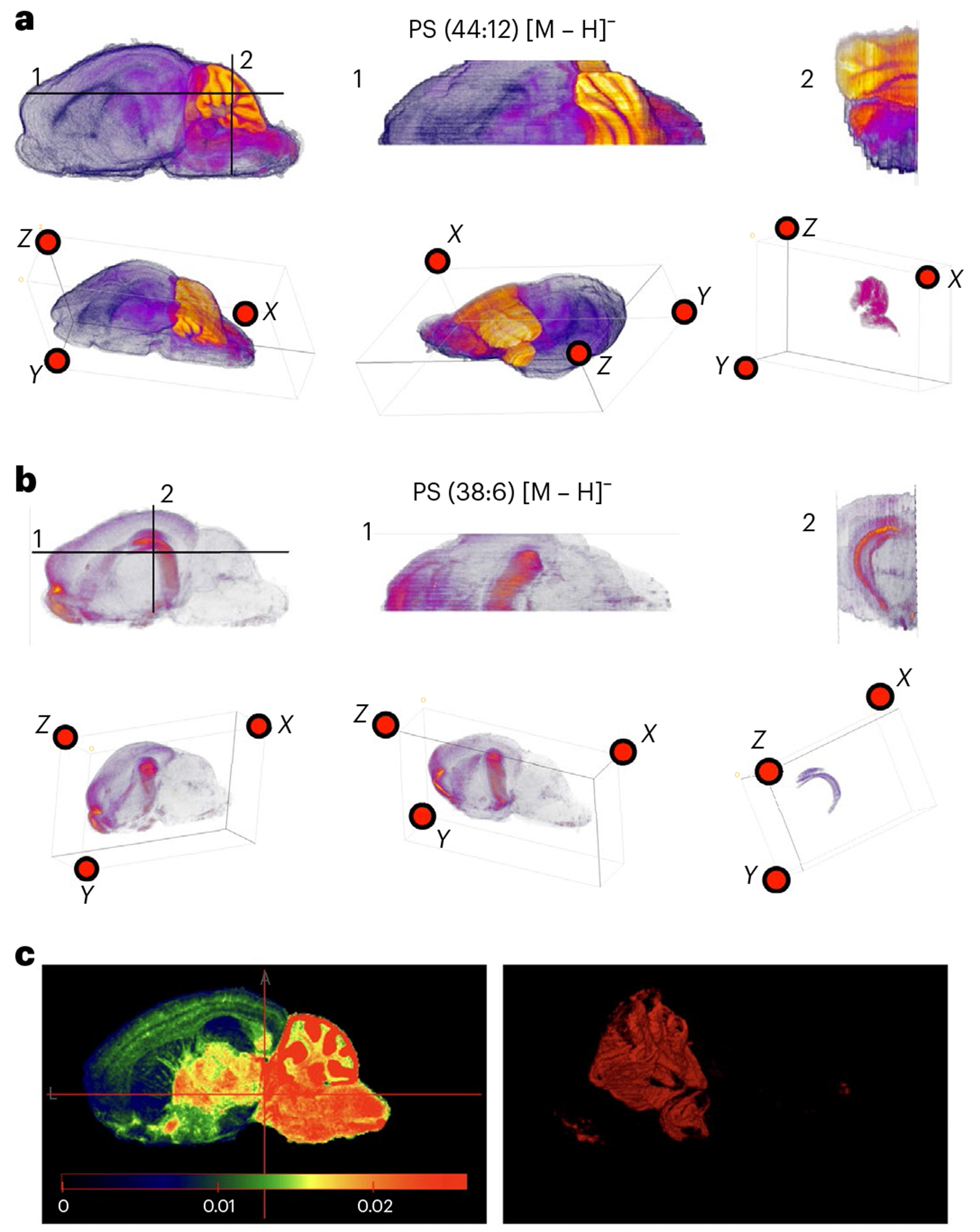
a, MetaVision3D rendering of PS 44:12 [M – H]− in 3D space. Top-down and frontal cross-sectional views are designated as 1 and 2 shown on the 2D side-view image. The 3D rendering is visualized by ImageJ using both projection mode and 3D fill of regions with high intensity of PS 44:12 [M – H]− in the cerebellum (Methods). b, MetaVision3D rendering of PS 38:6 [M – H]− in 3D space. Top-down and frontal cross-sectional views are designated as 1 and 2 shown on the 2D side-view image. The 3D rendering is visualized by ImageJ using both projection mode and 3D fill of regions with high intensity of PS 38:6 [M – H]− in the cerebellum (Methods). c, Screenshot of https://devmetavision3d.rc.ufl.edu/ and its functionalities.
Mapping gross and fine structures of brain in 3D
After examining metabolite distribution in 3D, we observed unique spatial patterns that correspond closely to both gross and fine anatomical structures of the mouse brain (Fig. 5 and Extended Data Fig. 8). Using the Nissl-stained sagittal brain section of the same plane from the Allen Brain Atlas as a guide, we identified several common brain structures based on metabolite distribution, with a particular emphasis on various lipid species. These structures include gross anatomical regions such as the fibrous tracks, isocortex, hindbrain, hippocampal formation, cerebellar cortex, ventricular system and cerebral nuclei, as well as fine cellular regions such as the granular layers of the hippocampus and cerebellum (Fig. 5a,b and Extended Data Fig. 8). By matching the spatial distributions of lipids observed in 2D MALDI imaging to the anatomical reference provided by the Allen Brain Atlas, we were able to delineate distinct brain regions and further map them into 3D space. For example, the fibrous tracks of the brain were defined by the unique spatial organization of several lipids, including LPE 20:1 [M – H]−, and rendering these lipids in 3D allowed us to visualize the volumetric distribution of not only the lipid species but also the structural organization of the fibrous tracks in 3D space (Fig. 5b–d). Other gross anatomical regions were similarly associated with specific lipid species, such as PE 38:6 [M – H]− and PE 36:2 [M – H]− in the isocortex, PS 44:12 [M – H]− in the hindbrain, PE 38:4 [M – H]− in the hippocampal region, PI 40:4 [M – H]− in the ventricular system, and LPE 20:4 [M – H]− in the cerebral nuclei (Extended Data Fig. 8). Notably, many lipid features were observed across multiple brain regions rather than being restricted to a single anatomical area, for example, PE 38:6 [M – H]− is pronounced in both the isocortex and the hippocampus (Extended Data Fig. 8), highlighting their shared metabolic significance and function.
Fig. 5 |. Anatomical structures and visualization of metabolite distributions in the mouse brain in 3D.

a, Gross anatomical regions of the mouse brain from the Allen Brain Atlas. b, Nissl-stained sagittal brain section from the Allen Brain Atlas and Allen Reference Atlas – Mouse Brain, highlighting fibrous tracks in red. c, Two-dimensional MALDI imaging of LPE 20:1 [M – H]−, showing a spatial distribution closely corresponding to the fibrous tracks. d, Three-dimensional rendering of LPE 20:1 [M – H]−, demonstrating the volumetric organization of the fibrous tracks. e, A Nissl-stained sagittal brain section highlighting the hippocampal formation and cerebellar cortex in red. f, Two-dimensional MALDI imaging of PI 38:5 [M – H]−, which mirrors the spatial distribution of the hippocampal formation and cerebellar cortex. g, A zoomed-in image of the cerebellar (Cere) granular layer and hippocampal (Hippo) granular layer, revealing elevated levels of PI 38:5 [M – H]− in these distinct cellular layers (indicated by arrows) compared with the Nissl-stained brain section from the Allen Brain Atlas. h, Three-dimensional volumetric visualization of the cerebellar granular layer and hippocampal granular layer as defined by PI 38:5 [M – H]−. Intensity scales for 2D images range from minimum (purple) to maximum (yellow/red), as indicated in the colour bar below c. Allen Mouse Brain Atlas, mouse.brain-map.org and atlas.brain-map.org.
In addition to brain gross structures, we also observed metabolites corresponding to fine cellular regions. For example, the three distinctive layers of cerebellum can be separated by PI 38:5 [M – H]− (granular layer), PS 44:12 PI 38:5 [M – H]− (molecular layer) and LPE 20:3 PI 38:5 [M – H]− (white matter tracks) (Fig. 5 and Extended Data Fig. 8). Furthermore, PI 38:5 [M – H]− is a lipid species enriched in both the hippocampus and cerebellum (Fig. 5e,f). Upon closer examination, its accumulation is highly localized to the granule cell layers of both of these regions (Fig. 5g). The granule cell layer of the hippocampus and cerebellum both consist of densely packed neuronal cell bodies, making them distinct fine structures of the brain. By gating the intensity of PI 38:5 [M – H]− to the 99th percentile using the Metavision3D platform, we can specifically map the 3D organization of these granule layers, providing a detailed volumetric representation (Fig. 5h). This demonstrates how 3D spatial metabolomics can be utilized to map and analyse both gross and fine brain structures, offering a deeper understanding of how these structures are coordinated and organized in 3D space, which can provide new insights into brain function.
Functional analysis of disease models in 3D
To increase the boarder impact of our online resource, we expanded the atlas to include additional set of wild-type (WT), 5xFAD and Gaa−/− mouse brains (6 months old, female). 5xFAD is a mouse of model of Alzheimer disease driven by β-amyloid plagues30, Gaa−/− is a model of paediatric glycogen storage disease with an increasing neurological focus31. Recent research has put altered brain metabolism at the centre of disease pathology for both mouse models32,33. Using the MetaVision3D workflow, we performed sequential MALDI imaging and rendered the brain metabolome in 3D for all three mouse models. These brains are presented in the online atlas side by side under the same intensity scale so we can observe changes in relative abundance of metabolites as well as their spatial distribution. For example, lipid accumulation has been reported in human patients with Alzheimer’s disease (AD) as well as in the 5xFAD mouse model34. In agreement with this notion, we observed increased fatty acids such LPE 22:4 [M – H]−, PE 38:5 [M – H]− and PE 38:4 [M – H]− but also mapped their spatial organization in 3D (Extended Data Fig. 9). Similarly, dysregulation in bioenergetics is also reported in the 5xFAD mouse model. In our 3D atlas, we observed a major reduction in ADP in the frontal cortex as well as cerebellum in the 5xFAD brain. It is interesting to note that the Gaa−/− mouse brain showed opposing trends for a number of metabolites compared with 5xFAD. For example, LPE 20:0 [M – H]−, PE 38:4 [M – H]− and ADP [M – H]− are dysregulated in the different direction compared with the 5xFAD brain (Extended Data Fig. 9). It is also worth noting that both WT brains provide similar 3D distribution for all metabolites, emphasizing the reproducibility of our method (Extended Data Fig. 7).
To further demonstrate the utility of our 3D atlas data to study brain metabolism, we performed proof-of-principle pathway enrichment analyses. The lipid PI 38:5 [M – H]− demonstrated spatial distribution in the brain; it is especially pronounced in the neuronal body layers of the hippocampus and cerebellum (Fig. 6 and Extended Data Fig. 10). Given that this lipid did not show changes between WT and 5xFAD brain, we extracted 3D pixels corresponding to the excitatory cell layers of hippocampus (Fig. 6b) and cerebellum (Extended Data Fig. 10b) separately. Our atlas is a high-dimensional dataset; therefore, each pixel within the 3D organization of the neuronal cell layers also contains the full metabolome data, including small-molecule metabolites and lipids. This can be done through the raw datasets as part of the resource. Once 3D pixels were extracted, we performed pathway enrichment using MetaboAnalyst for small-molecule metabolites and lipid ontology (LION) for lipid datasets (Fig. 6c and Extended Data Fig. 10c) by comparing the WT and 5xFAD brains. Top pathways highlighted by enrichment analysis for the hippocampus include ‘Warburg effect’, ‘aspartate metabolism’, ‘glutamate metabolism’, ‘low transition temperature’ and ‘low lateral diffusion’. Interestingly, not all pathways enriched in the hippocampal granule cell layer are present in the cerebellum. Pathways such as ‘transfer of acetyl group into mitochondria’, ‘citric acid cycle’, ‘lactose degradation’, ‘glycogenesis’ and ‘bilayer thickness’ are uniquely enriched in the granule cell layers of the cerebellum. Collectively, these data demonstrate the utility and application of the brain atlases provided by MetaVision3D.
Fig. 6 |. Pathway enrichment analysis of neuronal layers of the hippocampus in WT and 5xFAD mouse brains.

a, Two-dimensional slice and 3D rendered views of WT and 5xFAD mouse brains displaying the distribution of PI 38:5 in the hippocampus. A, anterior; L, lateral. b, Left: excitatory neuronal bodies of the hippocampus from a Nissl-stained sagittal brain section from the Allen Brain Atlas and Allen Reference Atlas – Mouse Brain. Allen Mouse Brain Atlas, mouse.brain-map.org and atlas.brain-map.org. Right: pixels corresponding to these regions were extracted for targeted analysis. c, Pathway enrichment analysis was performed on metabolomics (left) and lipidomics (right) datasets extracted from these pixels. Metabolomics pathway enrichment was conducted using MetaboAnalyst using the hypergeometric test and adjusted for multiple comparison (Bonferroni correction), highlighting key pathways such as the Warburg effect and aspartate metabolism based on −log10(P value). LION enrichment using the one-sided Kolmogorov–Smirnov test and adjusted for multiple comparison (Bonferroni correction) was performed using LION pathway analysis, identifying significant lipid categories, including diacylglycerophosphoglycerols and low-transition-temperature lipids based on −log10(P value).
Discussion
In this study, we introduced MetaVision3D, an AI-driven workflow designed to facilitate the generation of the 3D metabolome of tissues. MetaVision3D integrates a series of functionalities through computer vision—including normalization, alignment, imputation and interpolation to construct the spatial metabolome in 3D. Leveraging MetaVision3D, we constructed the first 3D metabolome of the mouse brain at the mesoscale. The innovation lies both in the precision and resolution of the spatial data and also in the workflow’s ability to compensate for experimental and technical variabilities inherent to MALDI imaging. The shift from conventional 2D representations to a 3D atlas marks a substantial technological leap, providing a great depth of metabolic insight that mirrors the complex 3D structure of the brain. The addition of AI transformed our ability to render serial sections to 3D space, as it was previously done through manual image orientation and stretching21–23 that limit the stack in the z axis. Metavision3D creates a push-button analytical pipeline that will process 3D rendering from MALDI imaging experiments. Finally, by moving into the third dimension, Metavision3D allows an understanding of metabolic distributions within the brain’s spatial architecture, setting a new standard for spatial metabolomics and opening new avenues for neurological research at mesoscale. Finally, to facilitate brain metabolism research, we are publishing the mouse brain metabolome atlas generated from MetaVision3D through an interactive website as well as a downloadable database.
The 3D metabolome offers a powerful approach to map both gross and fine structures of the brain with remarkable precision. To our surprise, metabolites display highly selective distributions across distinct brain regions. This selectivity is reflected in the ability of single lipid species to delineate gross anatomical regions when matched to the Allen Brain Atlas. For example, specific lipids such as PE 38:6 and PI 40:4 can distinctly define regions such as the isocortex, hindbrain, thalamus and hippocampus, highlighting the utility of metabolite mapping in tracing large-scale brain architecture. Interestingly, some lipid species span multiple distinct brain regions, such as the hindbrain and thalamus, or the isocortex and hippocampus. This overlap suggests functional significance, as the hindbrain and thalamus connection are critical for sensory relay and motor control35, while the isocortex and hippocampus connectivity play key roles in higher-order cognition and memory36. The presence of shared metabolites across these regions may indicate a conserved biochemical role necessary for their functional integration. Moreover, certain lipid species, such as PI 38:5, are uniquely enriched in fine cellular structures such as the granular layers of the hippocampus and cerebellum, which are composed of densely packed neuronal cell bodies. Leveraging this metabolic enrichment, we can trace the precise 3D organization and architecture of these neuronal layers in great detail. Interestingly, both regions have been shown through connection via neuronal circuitry37 and functional connectivity38 to be important for spatial cognition39. The observation that these regions may be linked through shared metabolites suggests the existence of a metabolic connectivity network linked to neuronal and functional connectivity in the brain. This hypothesis opens new avenues for understanding how distant brain regions coordinate through metabolic signals, potentially contributing to their integrated roles in brain function.
The brain exhibits intricate 3D architecture, yet most traditional studies rely on either coronal or sagittal sections, which inherently miss key regions. Coronal sections often fail to capture the full extent of the forebrain and hindbrain, while sagittal sections miss lateral structures such as the cortex or basal ganglia. As a result, these approaches are limited in their ability to comprehensively analyse the anatomy and metabolism of the brain in 3D. Metavision3D provides a transformative platform that integrates the entire 3D brain volume, enabling functional analysis across the entire structure. For example, we isolated pixels corresponding to the neuronal cell layers of both the hippocampus and cerebellum and extracted the full metabolome and lipidome from these layers in WT, 5xFAD (a model for AD) and GAA (a model for Pompe disease) mouse models. Our proof-of-concept analysis of these cell layers in 3D between WT and 5xFAD mice revealed significant metabolic pathway dysregulations, including the Warburg effect, aspartate metabolism and glutamate metabolism, which correspond to metabolic phenotypes associated with AD pathologies specific to these brain regions. In the future, these findings could guide the exploration of targeted therapeutic strategies aimed at correcting metabolic dysregulations in AD and other neurodegenerative diseases. Expanding this study to include a broader range of brain structures and disease models could uncover new insights into how brain metabolism is altered in pathology.
The Metavision3D atlas serves as a unique platform for visualizing and analysing the spatial metabolome in the context of gross and fine brain structures. However, to maximize its utility, this resource should be used in conjunction with other 3D atlases, such as the extensive resources offered by the Allen Brain Atlas40, which provides detailed anatomical references and molecular expression data. In addition, incorporating functional connectivity data from MRI studies can help to bridge metabolic networks with dynamic brain activity41, further enhancing our understanding of how metabolism relates to brain function and disease. The current Metavision3D atlas operates at a resolution of 50 μm, which, while highly informative for gross anatomical structures and regional metabolite distributions, does not yet capture the cellular identity of the brain. This limitation underscores the need for future advancements to integrate metabolomics datasets with emerging 3D transcriptomic resources, such as single-cell RNA sequencing in a spatially resolved context42. Such integration would allow researchers to link cellular identity and status directly to metabolic profiles, providing insights into how different cell types contribute to the overall metabolic landscape of the brain. This is particularly important for understanding cellular heterogeneity in both healthy and diseased states. Correlating cellular and metabolic data in this way could reveal how specific cell populations adapt their metabolic pathways during disease progression, offering new targets for therapeutic intervention. Expanding these capabilities will be critical for advancing our understanding not only of brain function and dysfunction but also of other systems such as cancer and other chronic diseases. By integrating 3D metabolomics with functional imaging and genetic analyses, we could establish a more comprehensive understanding of brain metabolism and its role in neurodegenerative diseases, providing critical insights for the development of precision medicine approaches to neurological disorders.
Methods
Chemicals, reagents and mouse models
HPLC-grade acetonitrile, ethanol, methanol, water, trifluoroacetic acid and N-(1-naphthyl) ethylenediamine dihydrochloride (NEDC) were purchased from Sigma-Aldrich. Mice were housed in climate-controlled environment with a 14 h (light)/10 h (dark) light/dark cycle with temperature (18–23 °C) and humidity (50–60%) control. Water and solid diet were provided ad libitum throughout the study (Tekad #2018). Female WT C57BL/6J and 5xFAD (034848-JAX) were purchased from The Jackson Laboratory. Female Gaa−/− strain (C57BL/6J background) was a gift from the late Dr Peter Roach laboratory at Indiana University. The University of Florida Institutional Animal Care and Use Committee has approved all of the animal procedures under the protocol number IACUC202200000586.
Sample collection and preparation
Mice were euthanized by cervical dislocation and decapitation. Immediately following euthanasia, the brains were surgically resected within 10 s. The brain tissue was first rinsed in 0.1× phosphate-buffered saline and subsequently rinsed twice with deionized water. The rinsed tissues were blotted dry, then slow-frozen over isopentane chilled with dry-ice for 7 min, according to previously established protocols1,2, to ensure tissue stability and optimal preservation of analytes. After freezing, the samples were stored at −80 °C for no more than 7 days until further processing.
MALDI MSI tissue preparation
The frozen tissues were sectioned by a cryostat chilled to −25 °C to prepare for cutting. A Leica CM1860 cryostat was utilized to obtain sagittal sections of 10 μm thickness. Tissues were mounted onto a frozen Leica chuck using optimal cutting temperature compound as a binding agent for sectioning. The brains were shaved until the target region (midline, sagittal view) was exposed. We obtained every fifth section, so the sections were exactly 50 μm apart, matching the spatial resolution of 50 μm of the MALDI imaging. The sections were then thaw-mounted onto glass slides, and the tissue samples were fixed by dehydration using a vacuum desiccator for 1 h. The slides were processed sequentially for small-molecule and lipid data acquisition by MALDI imaging.
Matrix application and MALDI imaging
Following an hour of vacuum desiccation, NEDC matrix was applied and sprayed using an HTX M5 pneumatic sprayer, using a matrix solvent of HPLC-grade methanol and water in a 70:30 mix. Then slides were sprayed with 7 mg ml−1 NEDC matrix in 70% methanol solvent, using 14 passes at a rate of 0.06 ml min−1, a 3 mm offset and a velocity of 1,200 mm min−1. The conditions were maintained at 30 °C and 10 psi, with a heated tray set at 50 °C. All MALDI MSI experiments were performed on a Bruker timsTOF fleX using a 46 μm × 46 μm laser raster to produce 50 μm × 50 μm pixels. Small-molecule metabolite imaging was performed in negative ion mode with the following instrument and laser settings: MS1 scan, 50 × 50 μm pixels from a 46 × 46 μm raster scan range, 90% laser power, 1 burst of 300 shots, 10,000 Hz frequency and an m/z range of 50–2,000. The MALDI laser was tuned remotely by a Bruker technician every Friday at 10:00. To obtain small molecules and lipids in the same run, additional parameters for tuning and calibration were implemented, including a MALDI plate offset of 30 V, deflection 1 delta of −60 V, funnel 1 radio frequency (RF) of 200 V peak-to-peak (Vpp), in-source collision-induced dissociation (isCID) energy of −0 eV, funnel 2 RF of 200 Vpp and multipole RF of 200 Vpp. The collision cell was optimized with a collision energy of 7 eV and collision RF of 700 Vpp, while the quadrupole was set at an ion energy of 5 eV with a low mass cut-off of 50 m/z. Ion mobility was disabled during acquisition to allow the detection of m/z below 300. The focus pre-time-of-flight region was configured with a transfer time of 80 μs and a prepulse storage time of 5 μs. Sweeping parameters included collision RF values ranging from 200 Vpp to 700 Vpp, transfer times of 20–80 μs and collision energies of 100–250%. Detection was conducted with focus mode enabled.
Peak annotations
MALDI imaging data analysis was conducted similarly to previous published methods43. We used MetaboScape software for exporting MS data acquired in negative ion mode into the .srd format, followed by data upload from Bruker SCiLS Software Solutions. T-ReX 2D algorithm was applied, focusing exclusively on MS data. Subsequent analysis incorporated parameters such as an intensity threshold of 500, speckle width and height of 3, and maximum of 200 speckles, with ion deconvolution targeting [M − H]−, [M + Cl]− and [M − H2O]− ions. Annotation used a hierarchical approach, starting with a curated list of 7,000 MS1 mammalian endogenous metabolites, followed by lipid identification using the MCube spectral library integrated into MetaboScape. Further annotation utilized a combination of in-house and public spectral libraries, including an in-house library of over 50,000 endogenous metabolites (curated through standards), the latest Human Metabolome Database Metabolite Library, MoNA, MassBank, FiehnLib LipidBlast library, MetaboBASE Personal Library 2023, the Bruker Sumner MetaboBASE and National Institute of Standards and Technology 2022. Annotation accuracy was ensured through stringent m/z tolerances (5–10 ppm), mSigma values (25–250) and comprehensive parallel library searches, with unannotated features explored via SmartFormula for molecular formula prediction. Results were exported in .mca format to SCiLS for peak width refinement and ion image quality assessment before final export in .csv format for 3D image construction. Full pixel-by-pixel datasets were exported using the R package as part of the SCiLS software package.
Overview of MetaVision3D
MetaVision3D, which removes off-tissue areas, contains the following modules: MetaNorm3D, for the normalization of intraslice signal variabilities; MetaAlign3D (a computer vision technique) for automated alignment; MetaImpute3D, an imputation step for reconstructing missing regions or gaps in corrupted tissue sections; MetaInterp3D, an interpolation algorithm to improve overall 3D rendering visualization; and MetaAtlas3D, a 3D mouse brain metabolome atlas in an interactive online database and web server.
Elimination of off-tissue areas
We exported a matrix-related peak that has higher intensity in off-tissue part and lower intensity in other tissue regions. Based on this peak, we created a binary mask and applied some morphological operations such as opening and closing to remove small objects, fill small gaps and smooth the boundaries of the mask. The functions morphology. area_opening() and morphology.area_closing() from Scikit-image41 were used for this part. This refined mask represents the off-tissue part, so the pixels overlap with this mask will be regarded as off-tissue pixels and excluded from subsequent 3D atlas construction.
MetaNorm3D
To mitigate the bias from multiple tissue sections, we developed the module MetaNorm3D to normalize the metabolite intensity in each section. The normalization strategy ensured a smoother transition of metabolite intensities between serial sections, which enhance the representation and visualization of the 3D slices. Specifically, we denote as the intensity vector for slice k and apply the section normalization as
| (1) |
where is the normalization factor, is the median of intensity values of slice k and is the vector of the medians for all K slices. The normalization step is implemented in custom module MetaNorm3D() in MetaVision3D Python toolkit.
MetaAlign3D
For each slice k, we obtain the number of unique x coordinates () and y coordinates () and put the slice contour into the rectangle () with x coordinates as the row and y coordinates as the column. However, as the sizes of slices are different, the shape of rectangles are also different. To synchronize all slices into the same coordinate systems, we perform a padding approach by extending the centre of each rectangle horizontally with size and vertically with size . and are set the same for all slices, but the choice of and requires the extension larger enough to incorporate k rectangles. Finally, the extended rectangle () is treated as the common coordinate system, where all are centralized in the coordinate system for the alignment in the next step. The centralized slice k is denoted as . We further use vectorization to representation all slices by denoting each slice as . All are made the same dimension, where the pixels outside are padding as 0. In this way, can be used for calculating ECC42 for slice alignment as follows.
MetaAlign3D aims to align all slices to minimize those geometric distortions without the need for additional histological images or atlases as the reference. Hereby, we developed MetaAlign3D, which is an algorithm to align multiple slices sequentially in the common coordinate system. For the sequential of tissue sections profiled by MALDI imaging in the tissue/organs (for example, 79 series brain sections from mouse hemibrain), MetaAlign3D starts from the largest brain section and performs the alignment in a sequential manner. Specifically, in the first iteration, the first slice, usually the largest one, is treated as a reference image (denoted as ), and the adjacent slice is treated as the warped image (denoted as ), which is the image that will undergo a transformation to align it with the reference image . A rigid body transformation (that is, Euclidean) is determined using an ECC function42,43 and applied to the warped image such that
| (2) |
where z is the coordinates in the reference image, is the transformation and p is the parameter vector. The alignment is driven by the function to maximize the ECC value between the warped image and the reference image. The optimal alignment is decided by the setting where the ECC value is maximized. Optimal transformation parameters were obtained by iteratively solving this objective function and then applying these transformation parameters to . In the next iteration, the corrected warped slice becomes the new reference image , and the next adjacent slice will become the new warped image . The iterations stop when all slices are finished aligning.
As the default setting, as all compounds have identical coordinates, we adopt the metabolite with the highest prevalence to calculate transformation parameters in . All remaining compounds share these parameters for alignment. The alignment can be easily tailored to include the information of multiple compounds by using meta-compounds, such as top principal components for compound–pixel dimension reduction. We implement both the manual slice fitting and alignment using OpenCV43 library and custom module Meta-Align3D() in MetaVision3D Python toolkit.
MetaImpute3D
Due to technical issues that may arise during the slicing process, some regions of the slices may be missing. To recover the metabolite intensity in the missing regions, we developed a functional module, named MetaImpute3D, to predict the metabolite intensity in the missing pixels for the targeted slice, which will enhance the continuity of 3D visualization and representation of the series slices. Based on the aligned 3D slices, MetaImpute3D performs two steps for the imputation. The first step of MetaImpute3D is to impute the missing pixels in the targeted slice by leveraging the nearby slices, and the second step is to refine the boundary between imputed regions and observed regions in the targeted slice.
Specifically, we denote the target slice as and the adjacent slices before and the slices after the target slice . As the adjacent slices are close to the target slice in anatomical region, they are more likely to share the similar metabolite intensity. We obtain the predicted metabolite intensity in the missing pixels by calculating the average non-zero metabolite intensity of aligned pixels in the adjacent two slices such as
| (3) |
where is the indices of neighbour slices and is the coordinate of a pixel. In default, because there is a low chance that four consecutive slices all have the same missing pixels. However, the window size can be easily adjusted case by case.
The second step of MetaImpute3D is to refine the boundary between the observed region and the imputed region in the target slice. There are two reasons for the refinement steps. First, the metabolite intensity of the observed regions is decreasing until zero intensity in the missing regions owing to technical bias. Second, there might be gaps between observed pixels and imputed pixels because the adjacent slices after the target slices might be smaller than the target slice. Due to the two reasons, we adopt cv.findContours() in OpenCV2 to detect the contour between imputed regions and the observed regions in the targeted slice and still use adjacent slice information to impute metabolite intensity for all pixels in the contour region. Similar to alignment, imputation is also a sequential process where each slice is checked and imputed sequentially. The whole imputation pipeline was implemented in Python using the custom module MetaImpute3D() in the MetaVision3D Python toolkit.
MetaInterp3D
In the original serial slices, there is a gap between each slice, which may cause large gaps in the 3D visualization. It is important to create an option step to create pseudo-slices to fill the gap for smoothing visualization in the -axis continuity and improve the overall accuracy of the 3D reconstruction. Specifically, we utilize linear interpolation to insert multiple phantom slices between the original adjacent slices. Suppose we want to insert a slice between slice and slice , where . The intensity value of pixel in is
| (4) |
In our case, we added two extra pseudo slices between each pair of adjacent slices. After insertion, the distance between the two 10-μm slices is reduced to 10 μm in the original data, and the thickness is reduced to 15 μm with no gap in 5xAD and WT data. The interpolation is performed using the Scipy4 library and MetaInterp3D() module in the MetaVision3D Python toolkit.
MetaAtlas3D
We produce the first 3D spatial metabolomics atlas of the mouse hemibrain using MetaAtlas3D (Fig. 2a). MetaAtlas3D data output is compatible with ImageJ, which researchers can utilize to visualize 3D models of individual metabolites. Importantly, we made this atlas accessible through a dual-platform approach: as an interactive website portal (https://metavision3d.rc.ufl.edu) and as a downloadable database. The input for the MetaAtlas3D is the 3D image in .nii format, which is the stack of the 2D slices generated from previous steps. To preserve the original brain shape while accommodating the insertion of interpolated slices (s slices), we adjusted the z-axis voxel dimension in the .nii file on the basis of the slice resolution (r; μm), slice thickness (h; μm) and the gap between adjacent slices (g; μm). The adjusted z-axis dimension is
| (5) |
The web-based platform offers a user-friendly interface where each metabolite is represented through both 2D slice transitions and 3D renderings with a customizable pixel intensity threshold. For a tutorial on how to use both ImageJ and online portal, please visit https://bit.ly/3T0T33T.
Evaluation metrics
To evaluate the performance of alignment and imputation, we use three metrics: ECC42, SSIM27 and MSE.
Suppose we have a pair of images and for the reference slice (before alignment or imputation) and the processed slice (after alignment or imputation) respectively, and and are vectors for representing and . The ECC is calculated as
| (6) |
where and are the zero-mean version of the vectors for and , respectively.
The SSIM is calculated as
| (7) |
where is the luminance comparison function, is the contrast comparison function and is the structure comparison function; , , are parameters used to adjust the weights of the three components.
The MSE is calculated as
| (8) |
We use the scikit-image1 library, OpenCV3 library, along with custom functions to calculate these metrics.
Metabolite pathway enrichment analysis and lipid ontology enrichment analysis
To investigate the differences between 5xAD and WT brains, we conducted metabolite enrichment analysis and LION enrichment analysis. We first used the created 3D atlas to roughly determine the brain regions of interest (ROIs). We then selected the central 2D slice of the 3D atlas as a reference to precisely define ROIs. Considering the 3D structural characteristics of the brain, we added extra space around the ROIs and broadcasted them to all other slices. Finally, we extracted the metabolite and lipid data from well-defined ROIs for enrichment analysis. In metabolite pathway enrichment analysis, we calculated the mean of intensity of each metabolite in the ROIs for both 5xAD and WT brains separately. Using these means, we computed the absolute value of log2 fold change of each metabolite in 5xAD relative to WT. All the metabolites with absolute log2 fold change greater than 0.5 were considered as input for MetaboAnalyst44 to perform pathway enrichment analysis using the Small Molecule Pathway Database (SMPDB)45. In MetaboAnalyst44, the hyperparametric distribution test was used to find significant pathways. We selected the top ten most enriched pathways to display in a barplot and a network. The network reflects the similarity between pathways, where pathways with more than 25% common metabolites are connected. In LION pathway enrichment analysis, the absolute log2 fold change of lipids was calculated in the same way as for metabolites. In LION/web46, all lipids were ranked by absolute log2 fold change and applicable LION terms were associated to the dataset. The distributions were compared with a uniform distribution using the Kolmogorov–Smirnov test. We still used a barplot and a network to visualize the ten most enriched LION terms. However, different from the previously used network, the network here was a hierarchical network presenting relationships between various lipid properties, classifications and functions.
Reporting summary
Further information on research design is available in the Nature Portfolio Reporting Summary linked to this article.
Extended Data
Extended Data Fig. 1 |. 2D MALDI heatmap images of serial mouse brain sagittal sections.
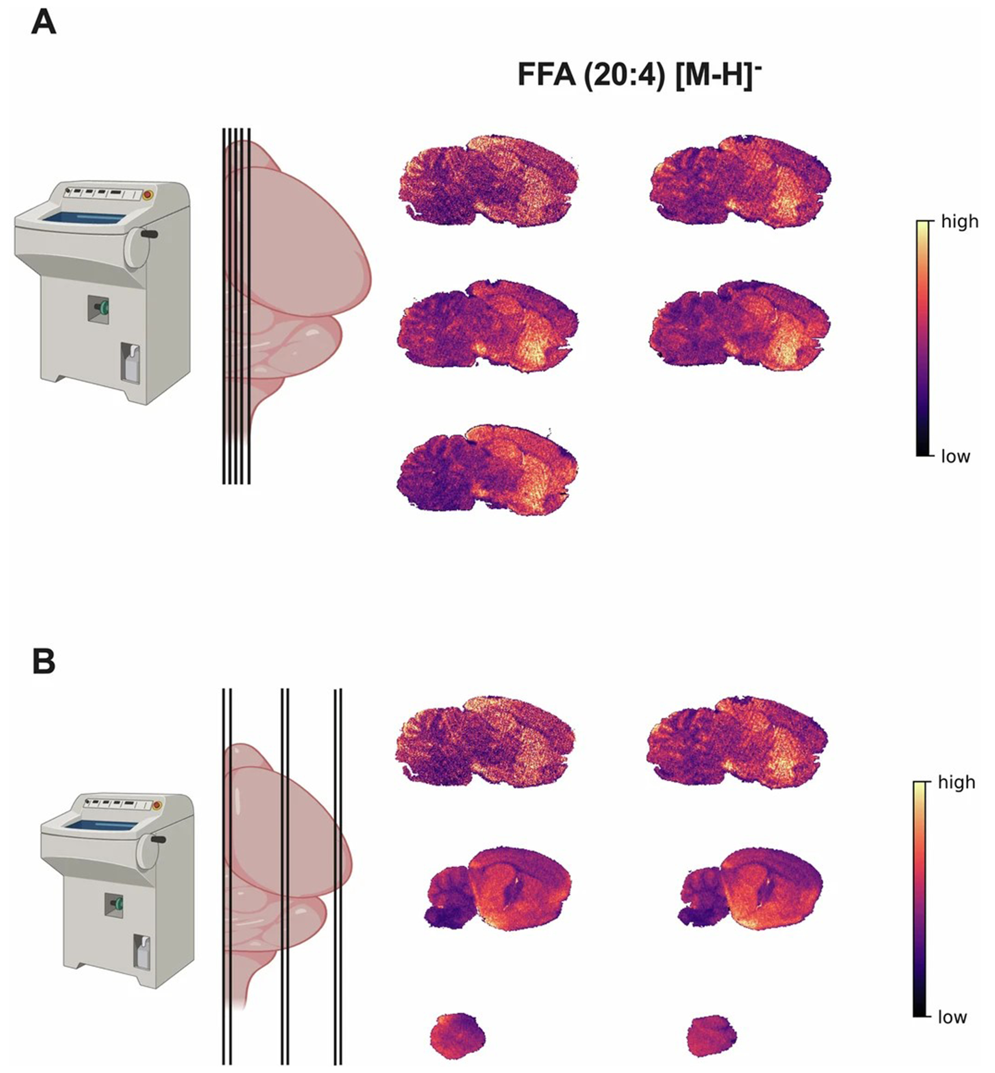
a. Schematic of five serial sagittal cut brain sections from the medial plane (left). Heatmap images for the spatial distribution of the free fatty acid (FFA) 20:4 in 2D for all five serial brain sections tested for alignment. b. Schematic of serial sagittal cut brain sections from the medial to posterior brain with different section sizes (left). Heatmap images for the spatial distribution of the free fatty acid (FFA) 20:4 in 2D for all six serial brain sections with different sizes tested for alignment.
Extended Data Fig. 2 |. Normalization of serial brain sections for 3D construction using MetaNorm3D.

a. Representative intensity distribution of PIP 38:4 among all 79 serial sections of the mouse sagittal hemi-brain. b. Representative intensity distribution of PIP 38:4 after slide normalization (see method) among all 79 serial sections of the mouse sagittal hemi-brain.
Extended Data Fig. 3 |. 2D MALDI heatmap images of serial mouse brain sagittal sections before and after normalization.

a. Heatmap images for the spatial distribution of PIP 38:4 in 2D for all 79 serial brain sections for 3D construction before and after normalization. Insert sections represents tissue sections with disparities in total abundance are zoomed in below. b. Heatmap images for the spatial distribution of PI 36:4 in 2D for all 79 serial brain sections for 3D construction before and after normalization. Insert sections represents tissue sections with disparities in total abundance are zoomed in below.
Extended Data Fig. 4 |. MetaImpute3D to fill in imperfections during sample handling.
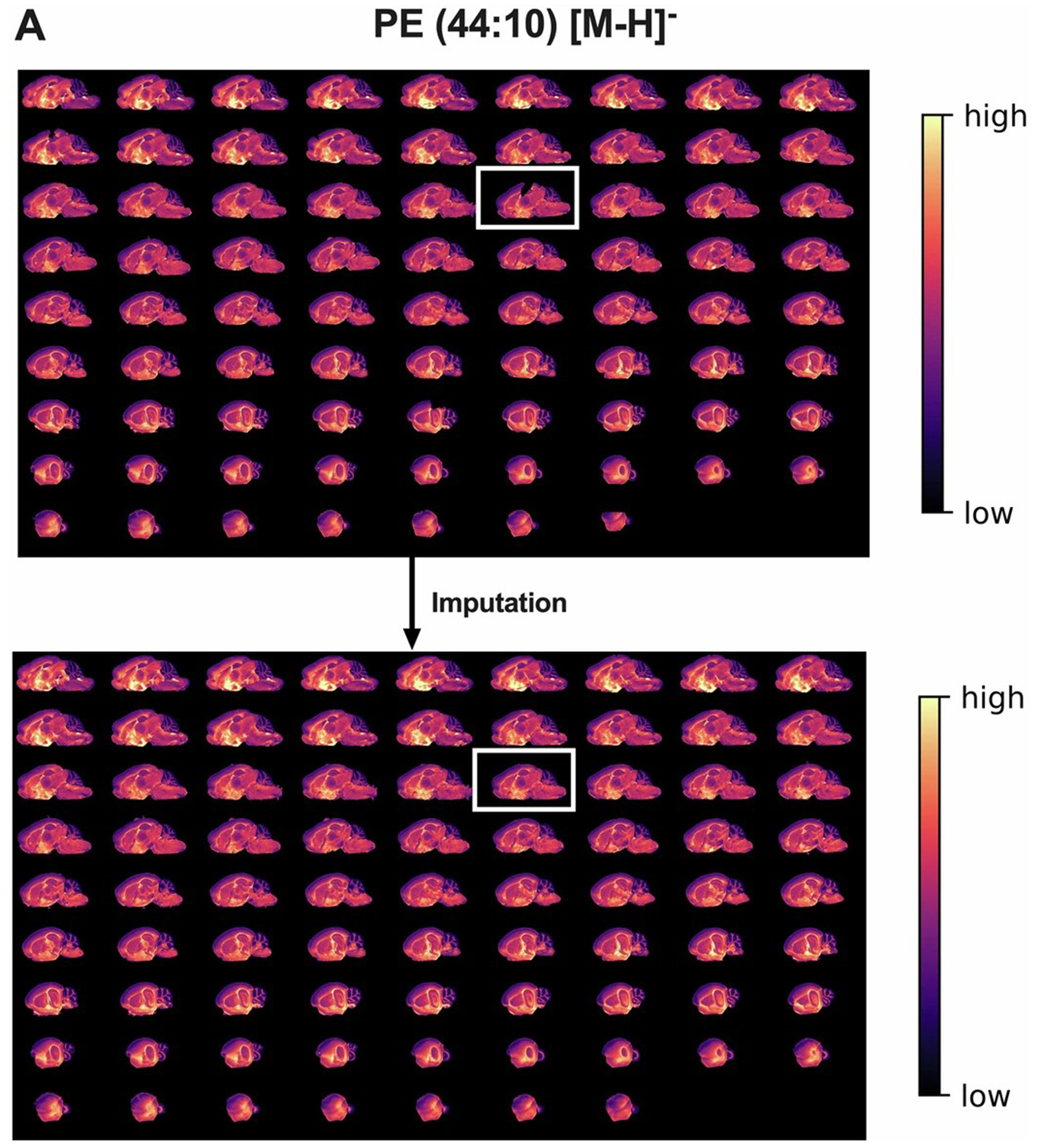
a. Heatmap images for the spatial distribution of PE 44:10 in 2D for all 79 serial brain sections for 3D after normalization, but before and after imputation of gaps in tissue. A representative tissue section after imputation is highlighted in the insert.
Extended Data Fig. 5 |. MetaInterp3D to fill in imperfections during sample handling.
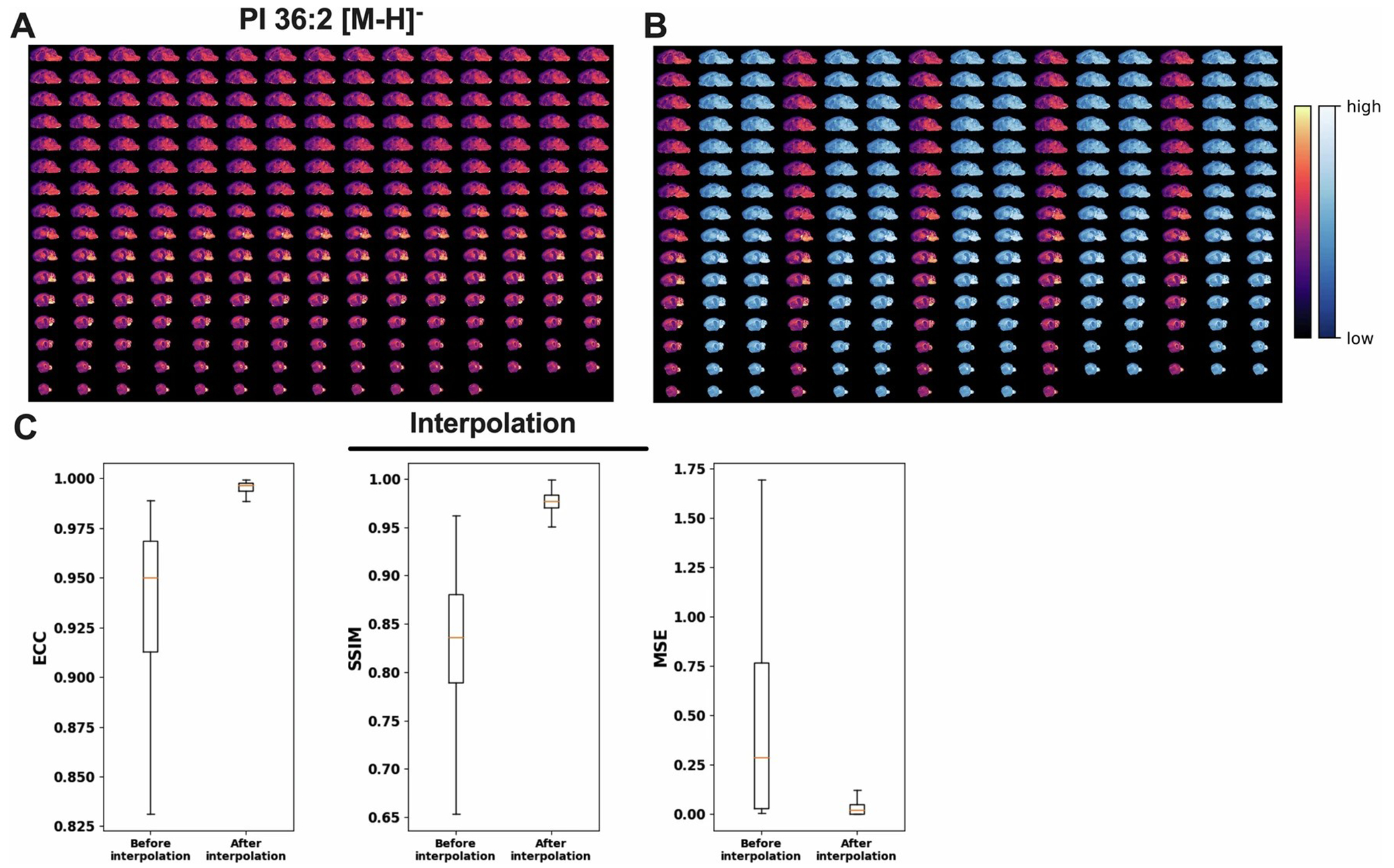
a. Representatives heatmap images for the spatial distribution of PI 36:2 in 2D for all 79 real and 158 phantom serial brain sections for 3D construction. b. same as a, except phantom sections are highlighted in green. c. Statistical measures of alignment and fit quality measured by enhanced correlation coefficient (ECC), structural similarity index measure (SSIM), and mean squared error (MSE) after interpolation (316 section). The box-and-whisker plot in panel d shows the median (line), interquartile range (box), and variability (whiskers extending to the maximum and minimum data points) n = 857 (11 different lipid class across 79 brain section) before interpolation and n = 2571 (11 different lipid class across 237 brain section).
Extended Data Fig. 6 |. Additional examples of spatial metabolome atlas of by MetaVision3D.

a. Front cross section and top-down view of fine brain anatomical structures of mouse brain cerebellum and hippocampal region in manual fit and after MetaVision3D framework. b and c. MetaVision3D rendering of PI 38:5 and PS 40:6 in 3D space. Top down (transverse) and front cross section (coronal) views are designated as 1, 2 or 3 shown on the 2D side view image. 3D rendering is visualized by ImageJ using both projection mode and 3D fill of regions with high intensity of both features.
Extended Data Fig. 7 |. Reproducibility of 3D lipid distribution in independent WT mouse brains.
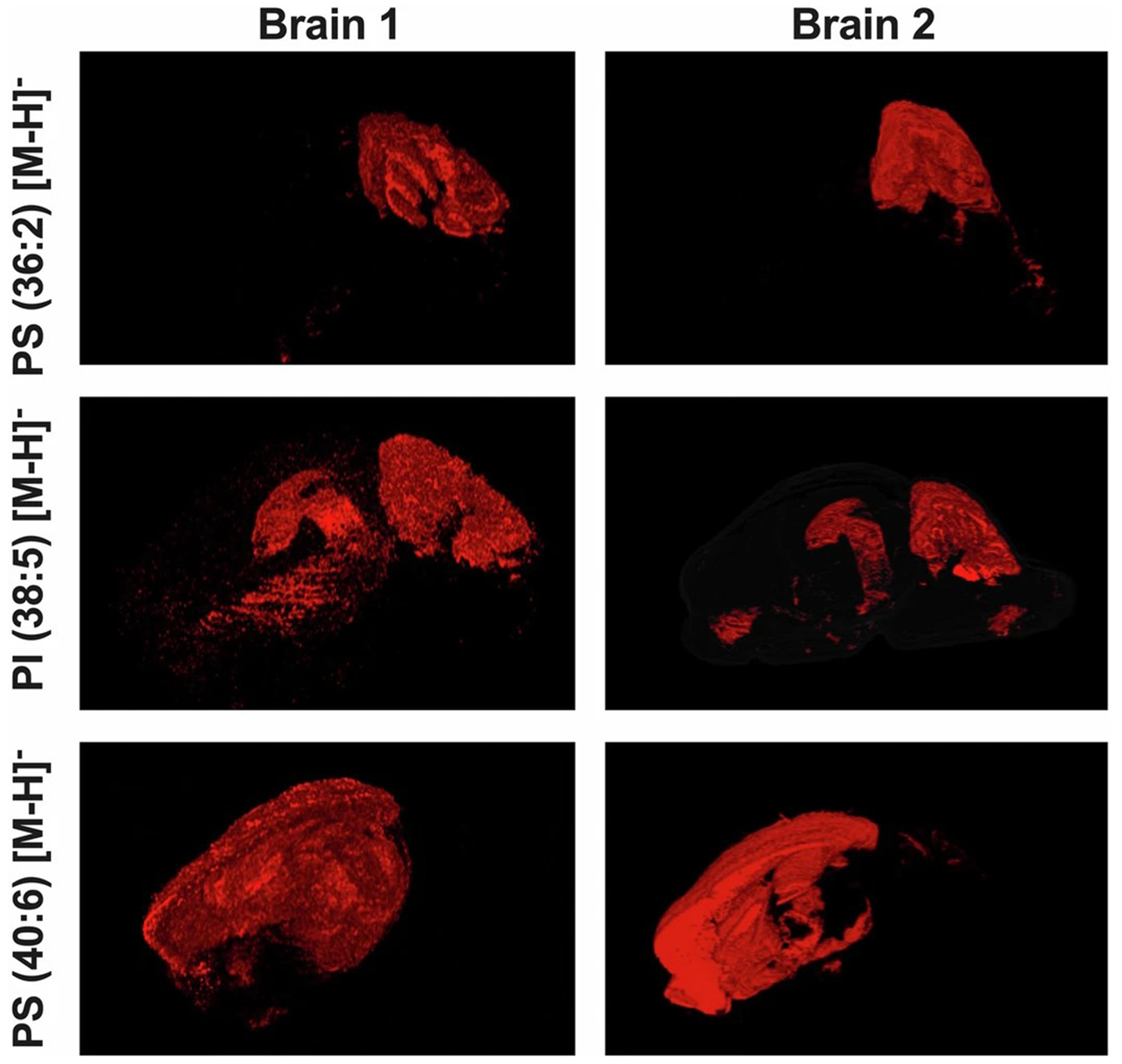
3D rendered views of two independent WT mouse brains (Brain 1 and Brain 2) showing the spatial distribution of three lipid species: PS 36:2, PI 38:5, and PS 40:6. The consistent patterns across the two brains demonstrate the reproducibility of lipid localization in the hippocampus and surrounding regions. 3D renderings are produced by MetaVision website.
Extended Data Fig. 8 |. 3D distribution of representative lipids highlighting anatomical regions in the mouse brain.

Representative images showing the spatial distribution of specific lipid species in mouse brain regions. (Left) Nissl-stained sagittal brain section of the same plane from the Allen Brain Atlas and Allen Reference Atlas, – Mouse Brain, Allen Mouse Brain Atlas, mouse.brain-map.org and atlas.brain-map.org with regions of interest highlighted in red, including the isocortex, hindbrain, cerebellar molecular layer, hippocampal region, ventricular system, and cerebral nuclei. (Middle) Sagittal plane images obtained using 2D MALDI imaging from our study, illustrating the relative abundance and localization of the indicated lipid species. (Right) 3D visualization of lipid distributions, highlighting the top 1% highest intensity pixels to resolve their spatial organization. Lipid species are annotated above each row: PE 38:6 [M-H]−, PE 36:2 [M-H]−, PS 44:12 [M-H]−, PE 38:4 [M-H]−, PI 40:4 [M-H]−, and LPE 20:4 [M-H]−. Intensity scales range from minimum (purple) to maximum (yellow/red) as depicted in the bottom scale bar.
Extended Data Fig. 9 |. Comparative analysis of lipid and metabolite distribution in WT, 5xFAD, and Gaa−/− mouse brains.
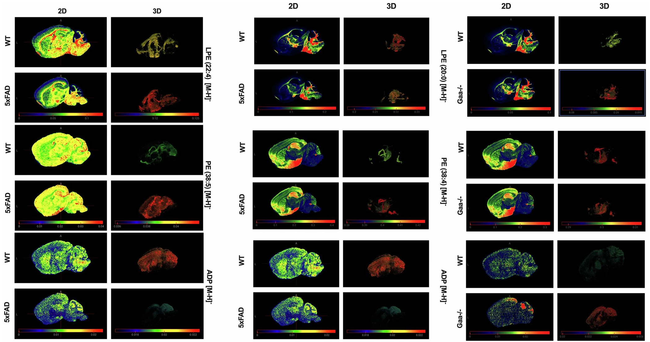
2D slice and 3D rendered views showing the distribution of specific lipids (LPE 22:4, PE 38:5, LPE 20:0, PE 38:4) and metabolites (ADP) across different mouse models: WT, 5xFAD (Alzheimer’s disease model), and Gaa−/−. The left panel compares WT and 5xFAD brains, while the right panel compares WT and Gaa−/− brains. The color scales indicate the relative intensity of the lipid/metabolite signals, illustrating differences in spatial distribution between the genotypes. These comparisons highlight alterations in brain metabolism and lipid composition associated with Alzheimer’s disease and GAA deficiency.
Extended Data Fig. 10 |. Pathway enrichment analysis of neuronal layers of the cerebellum in WT and 5xFAD mouse brains.

a. 2D slice and 3D rendered views of WT and 5xFAD mouse brains displaying the distribution of phosphatidylinositol (PI) 38:5 in the hippocampus and cerebellum. b. The excitatory neuronal bodies of the cerebellum from a Nissl-stained sagittal brain section from the Allen Brain Atlas and Allen Reference Atlas, – Mouse Brain, Allen Mouse Brain Atlas, mouse.brain-map.org and atlas.brain-map.org (left) and pixels corresponding to these regions were extracted (right) for targeted analysis. c. Pathway enrichment analysis was performed on metabolomics (left) and lipidomics (right) datasets extracted from these pixels. Metabolomics pathway enrichment was conducted using MetaboAnalyst using the hypergeometric test and adjusted for multiple comparison (bonferroni correction) highlighting key pathways such as the transfer of acetyl groups into mitochondria, the Warburg effect, and the citric acid cycle based on −log10(pvalue). Lipid ontology enrichment using the one-sided Kolmogorov-Smirnov test and adjusted for multiple comparison (bonferroni correction) was performed using Lipid Ontology (LION) pathway analysis, identifying significant lipid categories related to bilayer thickness and lateral diffusion properties based on −log10(pvalue).
Supplementary Material
Acknowledgements
This study was supported by National Institutes of Health (NIH) grants R01AG066653, R01CA266004, R01AG078702, 1R01CA288696 and RM1NS133593 to R.C.S., R35NS116824 to M.S.G., R35GM142701 to L.C., T32HL134621 to H.A.C. and 1R01NS127280 to N.N.Y.
Competing interests
R.C.S. has research support and received consultancy fees from Maze Therapeutics. R.C.S. is a member of the Medical Advisory Board for Little Warrior Foundation. M.S.G. received research support and research compounds from Maze Therapeutics, Valerion Therapeutics and Ionis Pharmaceuticals. M.S.G. also received a consultancy fee from Maze Therapeutics, PTC Therapeutics and the Glut1-Deficiency Syndrome Foundation. The other authors declare no competing interests.
Footnotes
Extended data is available for this paper at https://doi.org/10.1038/s42255-025-01242-9.
Supplementary information The online version contains supplementary material available at https://doi.org/10.1038/s42255-025-01242-9.
Code availability
Python code for the entire MetaVision3D framework and test dataset is available via GitHub at https://github.com/XinBiostats/MetaVision3D and via Zenodo at https://doi.org/10.5281/zenodo.14213133 (ref. 48).
Data availability
The 3D atlas of the brain metabolome and downloadable files are available at https://metavision3d.rc.ufl.edu. Raw data in .csv format are available via Zenodo at https://doi.org/10.5281/zenodo.14212426 (ref. 47) and in imzML format are available at https://sunlabresources.rc.ufl.edu. Tutorials on how to use the online atlas and ImageJ are available at https://www.youtube.com/channel/UC5tUZiZHCjS33Un4yxfIWdw. Source data are provided with this paper.
References
- 1.Moses L & Pachter L Museum of spatial transcriptomics. Nat. Methods 19, 534–546 (2022). [DOI] [PubMed] [Google Scholar]
- 2.Rao A, Barkley D, França GS & Yanai I Exploring tissue architecture using spatial transcriptomics. Nature 596, 211–220 (2021). [DOI] [PMC free article] [PubMed] [Google Scholar]
- 3.Bendall SC et al. Single-cell mass cytometry of differential immune and drug responses across a human hematopoietic continuum. Science 332, 687–696 (2011). [DOI] [PMC free article] [PubMed] [Google Scholar]
- 4.Angelo M. et al. Multiplexed ion beam imaging of human breast tumors. Nat. Med 20, 436–442 (2014). [DOI] [PMC free article] [PubMed] [Google Scholar]
- 5.Rappez L. et al. SpaceM reveals metabolic states of single cells. Nat. Methods 18, 799–805 (2021). [DOI] [PMC free article] [PubMed] [Google Scholar]
- 6.Alexandrov T. Spatial metabolomics: from a niche field towards a driver of innovation. Nat. Metab 5, 1443–1445 (2023). [DOI] [PubMed] [Google Scholar]
- 7.Wang L. et al. Spatially resolved isotope tracing reveals tissue metabolic activity. Nat. Methods 19, 223–230 (2022). [DOI] [PMC free article] [PubMed] [Google Scholar]
- 8.Schwaiger-Haber M. et al. Using mass spectrometry imaging to map fluxes quantitatively in the tumor ecosystem. Nat. Commun 14, 2876 (2023). [DOI] [PMC free article] [PubMed] [Google Scholar]
- 9.Zhang H. et al. Single-cell lipidomics enabled by dual-polarity ionization and ion mobility-mass spectrometry imaging. Nat. Commun 14, 5185 (2023). [DOI] [PMC free article] [PubMed] [Google Scholar]
- 10.Li Z. et al. Single-cell lipidomics with high structural specificity by mass spectrometry. Nat. Commun 12, 2869 (2021). [DOI] [PMC free article] [PubMed] [Google Scholar]
- 11.Young LE et al. In situ mass spectrometry imaging reveals heterogeneous glycogen stores in human normal and cancerous tissues. EMBO Mol. Med 14, e16029 (2022). [DOI] [PMC free article] [PubMed] [Google Scholar]
- 12.Sun RC et al. Brain glycogen serves as a critical glucosamine cache required for protein glycosylation. Cell Metab. 33, 1404–1417 (2021). [DOI] [PMC free article] [PubMed] [Google Scholar]
- 13.Harrison AC et al. Spatial metabolome lipidome and glycome from a single brain section. Preprint at bioRxiv 10.1101/2023.07.22.550155 (2023). [DOI] [Google Scholar]
- 14.Vicari M. et al. Spatial multimodal analysis of transcriptomes and metabolomes in tissues. Nat. Biotechnol 42, 1046–1050 (2024). [DOI] [PMC free article] [PubMed] [Google Scholar]
- 15.Luo L. et al. Spatial metabolomics reveals skeletal myofiber subtypes. Sci. Adv 9, eadd0455 (2023). [DOI] [PMC free article] [PubMed] [Google Scholar]
- 16.He Y. et al. Prosaposin maintains lipid homeostasis in dopamine neurons and counteracts experimental parkinsonism in rodents. Nat. Commun 14, 5804 (2023). [DOI] [PMC free article] [PubMed] [Google Scholar]
- 17.Conroy LR et al. Spatial metabolomics reveals glycogen as an actionable target for pulmonary fibrosis. Nat. Commun 14, 2759 (2023). [DOI] [PMC free article] [PubMed] [Google Scholar]
- 18.Xia C-R, Cao Z-J, Tu X-M & Gao G Spatial-linked alignment tool (SLAT) for aligning heterogenous slices. Nat. Commun 14, 7236 (2023). [DOI] [PMC free article] [PubMed] [Google Scholar]
- 19.Zeira R, Land M, Strzalkowski A & Raphael BJ Alignment and integration of spatial transcriptomics data. Nat. Methods 19, 567–575 (2022). [DOI] [PMC free article] [PubMed] [Google Scholar]
- 20.Zhou X, Dong K & Zhang S Integrating spatial transcriptomics data across different conditions, technologies and developmental stages. Nat. Comput. Sci 3, 894–906 (2023). [DOI] [PubMed] [Google Scholar]
- 21.Andersson M, Groseclose MR, Deutch AY & Caprioli RM Imaging mass spectrometry of proteins and peptides: 3D volume reconstruction. Nat. Methods 5, 101–108 (2008). [DOI] [PubMed] [Google Scholar]
- 22.Trede D. et al. Exploring three-dimensional matrix-assisted laser desorption/ionization imaging mass spectrometry data: three-dimensional spatial segmentation of mouse kidney. Anal. Chem 84, 6079–6087 (2012). [DOI] [PubMed] [Google Scholar]
- 23.Giordano S. et al. 3D mass spectrometry imaging reveals a very heterogeneous drug distribution in tumors. Sci. Rep 6, 37027 (2016). [DOI] [PMC free article] [PubMed] [Google Scholar]
- 24.Alexandrov T. Spatial metabolomics and imaging mass spectrometry in the age of artificial intelligence. Annu. Rev. Biomed. Data Sci 3, 61–87 (2020). [DOI] [PMC free article] [PubMed] [Google Scholar]
- 25.Cai K. et al. Magnetic resonance imaging of glutamate. Nat. Med 18, 302–306 (2012). [DOI] [PMC free article] [PubMed] [Google Scholar]
- 26.Evangelidis GD & Psarakis EZ Parametric image alignment using enhanced correlation coefficient maximization. IEEE Trans. Pattern Anal. Mach. Intell 30, 1858–1865 (2008). [DOI] [PubMed] [Google Scholar]
- 27.Brunet D, Vrscay ER & Wang Z On the mathematical properties of the structural similarity index. IEEE Trans. Image Process 21, 1488–1499 (2011). [DOI] [PubMed] [Google Scholar]
- 28.Wang Z & Bovik AC Mean squared error: love it or leave it? A new look at signal fidelity measures. IEEE Signal Process. Mag 26, 98–117 (2009). [Google Scholar]
- 29.Schneider CA, Rasband WS & Eliceiri KW NIH Image to ImageJ: 25 years of image analysis. Nat. Methods 9, 671–675 (2012). [DOI] [PMC free article] [PubMed] [Google Scholar]
- 30.Eimer WA & Vassar R Neuron loss in the 5XFAD mouse model of Alzheimer’s disease correlates with intraneuronal Aβ 42 accumulation and caspase-3 activation. Mol. Neurodegen 8, 1–12 (2013). [DOI] [PMC free article] [PubMed] [Google Scholar]
- 31.Leon-Astudillo C. et al. Current avenues of gene therapy in Pompe disease. Curr. Opin. Neurol 36, 464–473 (2023). [DOI] [PMC free article] [PubMed] [Google Scholar]
- 32.Andersen JV et al. Hippocampal disruptions of synaptic and astrocyte metabolism are primary events of early amyloid pathology in the 5xFAD mouse model of Alzheimer’s disease. Cell Death Dis. 12, 954 (2021). [DOI] [PMC free article] [PubMed] [Google Scholar]
- 33.Ullman JC et al. Small-molecule inhibition of glycogen synthase 1 for the treatment of Pompe disease and other glycogen storage disorders. Sci. Transl. Med 16, eadf1691 (2024). [DOI] [PMC free article] [PubMed] [Google Scholar]
- 34.Kaya I. et al. Spatial lipidomics reveals region and long chain base specific accumulations of monosialogangliosides in amyloid plaques in familial Alzheimer’s disease mice (5xFAD) brain. ACS Chem. Neurosci 11, 14–24 (2020). [DOI] [PubMed] [Google Scholar]
- 35.Antón-Bolaños N, Espinosa A & López-Bendito G Developmental interactions between thalamus and cortex: a true love reciprocal story. Curr. Opin. Neurobiol 52, 33–41 (2018). [DOI] [PMC free article] [PubMed] [Google Scholar]
- 36.Yao Z. et al. A taxonomy of transcriptomic cell types across the isocortex and hippocampal formation. Cell 184, 3222–3241.e3226 (2020). [DOI] [PMC free article] [PubMed] [Google Scholar]
- 37.Bohne P, Schwarz MK, Herlitze S & Mark MD A new projection from the deep cerebellar nuclei to the hippocampus via the ventrolateral and laterodorsal thalamus in mice. Front. Neural Circuits 13, 51 (2019). [DOI] [PMC free article] [PubMed] [Google Scholar]
- 38.Yu WJ & Krook-Magnuson E Cognitive collaborations: bidirectional functional connectivity between the cerebellum and the hippocampus. Front. Syst. Neurosci 9, 177 (2015). [DOI] [PMC free article] [PubMed] [Google Scholar]
- 39.Watson TC et al. Anatomical and physiological foundations of cerebello-hippocampal interaction. eLife 8, e41896 (2018). [DOI] [PMC free article] [PubMed] [Google Scholar]
- 40.Oh SW et al. A mesoscale connectome of the mouse brain. Nature 508, 207–214 (2014). [DOI] [PMC free article] [PubMed] [Google Scholar]
- 41.Nasiriavanaki M. et al. High-resolution photoacoustic tomography of resting-state functional connectivity in the mouse brain. Proc. Natl Acad. Sci. USA 111, 21–26 (2013). [DOI] [PMC free article] [PubMed] [Google Scholar]
- 42.Shi H. et al. Spatial atlas of the mouse central nervous system at molecular resolution. Nature 622, 552–561 (2023). [DOI] [PMC free article] [PubMed] [Google Scholar]
- 43.Nunes JB et al. Integration of mass cytometry and mass spectrometry imaging for spatially resolved single-cell metabolic profiling. Nat. Methods 21, 1796–1800 (2024). [DOI] [PMC free article] [PubMed] [Google Scholar]
- 44.Xia J & Wishart DS Using MetaboAnalyst 3.0 for comprehensive metabolomics data analysis. Curr. Protoc. Bioinformatics 55, 14.10.1–14.10.91 (2016). [DOI] [PubMed] [Google Scholar]
- 45.Jewison T. et al. SMPDB 2.0: big improvements to the Small Molecule Pathway Database. Nucleic Acids Res. 42, D478–D484 (2014). [DOI] [PMC free article] [PubMed] [Google Scholar]
- 46.Molenaar MR et al. LION/web: a web-based ontology enrichment tool for lipidomic data analysis. Gigascience 8, giz061 (2019). [DOI] [PMC free article] [PubMed] [Google Scholar]
- 47.Ma X. MetaVision3D: automated framework for the generation of spatial metabolome atlas in 3D | MALDI data. Zenodo 10.5281/zenodo.14212426 (2024). [DOI] [Google Scholar]
- 48.Ma X. XinBiostats/MetaVision3D: version 1.0.0. Zenodo 10.5281/zenodo.14213133 (2024). [DOI] [Google Scholar]
Associated Data
This section collects any data citations, data availability statements, or supplementary materials included in this article.
Supplementary Materials
Data Availability Statement
The 3D atlas of the brain metabolome and downloadable files are available at https://metavision3d.rc.ufl.edu. Raw data in .csv format are available via Zenodo at https://doi.org/10.5281/zenodo.14212426 (ref. 47) and in imzML format are available at https://sunlabresources.rc.ufl.edu. Tutorials on how to use the online atlas and ImageJ are available at https://www.youtube.com/channel/UC5tUZiZHCjS33Un4yxfIWdw. Source data are provided with this paper.