Do the wealthy have a health advantage? Cardiovascular disease risk factors and wealth

Abstract

The use of wealth as a measure of socioeconomic status (SES) remains uncommon in epidemiological studies. When used, wealth is often measured crudely and at a single point in time. Our study explores the relationship between wealth and three cardiovascular disease (CVD) risk factors (smoking, obesity and hypertension) in a US population. We improve upon existing literature by using a detailed and validated measure of wealth in a longitudinal setting. We used four waves of data from the Panel Study of Income Dynamics (PSID) collected between 1999 and 2005. Inverse probability weights were employed to control for time-varying confounding and to estimate both relative (risk ratio) and absolute (risk difference) measures of effect. Wealth was defined as inflation-adjusted net worth and specified as a six category variable: one category for those with less than or equal to zero wealth and quintiles of positive wealth. After adjusting for income and other time-varying confounders, as well as baseline covariates, the risk of becoming obese was inversely related to wealth. There was a 40%–89% higher risk of becoming obese among the less wealthy relative to the wealthiest quintile and 11 to 25 excess cases (per 1000 persons) among the less wealthy groups over six years of follow up. Smoking initiation had similar but more moderate effects; risk ratios and differences both revealed a smaller magnitude of effect compared to obesity. Of the three CVD risk factors examined here, hypertension incidence had the weakest association with wealth, showing a smaller increased risk and fewer excess cases among the less wealthy groups. In conclusion, this study found a strong inverse association between wealth and obesity incidence, a moderate inverse association between wealth and smoking initiation and a weak inverse association between wealth and hypertension incidence after controlling for income and other time-varying confounders.

Introduction

The goal of this study was to explore whether less wealthy individuals have a higher risk of becoming obese, smokers or hypertensive. In epidemiological studies the use of wealth as a measure of socioeconomic status (SES) is uncommon. Wealth is defined as the stockpile of financial resources amassed over the lifetime, while income is the flow of resources into the household at any given point in time (Keister, 2000; Shapiro & Wolff, 2001).

There are several advantages to using wealth as a measure of SES. First, since it is less subject to fluctuations over one’s lifetime than income, wealth is often a more stable measure of SES. Since wealth is often inherited over the generations it reflects a historical accumulation of assets. Second, wealth may be a better measure of social hierarchy compared to other SES measures (Wilkinson, 1999). In addition to being an economic indicator, wealth buys political power, social prestige, and educational and occupational opportunities that income alone may not allow (Keister, 2000; Shapiro & Wolff, 2001). That is, wealth encompasses economic circumstances as well as prestige and status.

Finally, wealth may be a better measure of one’s economic situation at various points in the life course. For example, during times of unemployment or illness when income is lost, wealth may help maintain living standards. During these times, measures of employment status or income may misrepresent an individual’s economic situation. Some studies have shown that SES measures are not interchangeable; instead they may work through different mechanisms at different times in the life course (Braveman et al., 2005; Demakakos, Nazroo, Breeze, & Marmot, 2008). For example, wealth may be an especially good SES measure for older populations, when income is limited or absent (Keister, 2000; Pollack et al., 2007). In fact, several studies have shown a strong association between wealth and health in the elderly population (Cagney & Lauderdale, 2002; Menchik, 1993; Smith & Kington, 1997). Given these examples, it is easy to understand how wealth can work independently of income to impact health (Pollack et al., 2007).

Wealth is not often used in health studies because it is difficult to measure effectively. A thorough assessment of wealth would require asking several sensitive questions about the value of personal property, debt and financial instruments. Since wealth data are self-reported and difficult to validate, the possibility of poor measurement exists. Interestingly, the underestimation of assets by the wealthiest Americans has limited our ability to understand the true disparity in wealth that exists in the US (Wolff, 1995). In the health literature, measures of wealth are not consistent and are sometimes simplistic; thus making comparisons across studies difficult and masking potential associations between wealth and health outcomes (Pollack et al., 2007).

Most past studies used cross-sectional data to explore the relationship between wealth and CVD risk factors (Avendano, Glymour, Banks, & Mackenbach, 2009; Demakakos et al., 2008; Fonda, Fultz, Jenkins, Wheeler, & Wray, 2004; Kennickell, 2008; Kington & Smith, 1997; Laaksonen, Rahkonen, Karvonen, & Lahelma, 2005; Munster, Ruger, Ochsmann, Letzel, & Toschke, 2009; Robert & Reither, 2004; Rooks et al., 2002; Schaap, van Agt, & Kunst, 2008; Schoenbaum & Waidmann, 1997; Siahpush, Borland, & Scollo, 2002). Our study of wealth and CVD risk factors improves upon the existing literature by using a thorough and reliable measure of wealth (Curtin, Juster, & Morgan, 1989) from a longitudinal study, the Panel Study of Income Dynamics (PSID). Our choice of PSID was motivated not only by its detailed wealth measurement, but also by a desire to evaluate the wealth–health relationship in a non-elderly adult US population. Much work has looked at wealth and CVD risk factors in the elderly (Adams, Hurd, McFadden, Merrill, & Ribeiro, 2003; Avendano et al., 2009; Demakakos et al., 2008; Fonda et al., 2004; Kington & Smith, 1997; Rooks et al., 2002; Schoenbaum & Waidmann, 1997), but fewer studies have examined the effect of wealth on health in a population of established adults.

Methods

Data

PSID is a longitudinal study of the US population which began in 1968 and continues today. Currently data are collected biennially. Although PSID was designed to be representative of the non-institutionalized, civilian US population, survey weights were not used in this study. The use of survey weights would have complicated the analytic method we used which also relies on analytic weights. Thus results from this study are not generalizable to the broader US population. Much has been written about the design and content of the PSID elsewhere (An overview of the panel study of income dynamics, 2009). Data for this study came from the 1999, 2001, 2003 and 2005 waves of the PSID. Regular data collection of the health module began in 1999 and has continued in each wave since. Health questions were asked only of the head of household and his/her partner.

Measures

Health outcomes

The three health outcomes examined in this study, obesity, smoking and hypertension, were self-reported. Obesity was derived from self-reported height and weight and was classified using a body mass index of 30 or higher. Smoking status was derived from a series of questions on smoking behavior allowing participants to be classified as current, former or never smokers. Lastly, hypertension was ascertained from a single question, “Has a doctor ever told you that you have or had high blood pressure or hypertension”.

Wealth

Family wealth was defined as total net worth, which includes the value of one’s primary home, farm or business assets, checking or savings accounts, vehicles, second homes, stocks and bonds. Debt was subtracted from these assets. All wealth data were adjusted for inflation using the 2001 consumer price index. Wealth was specified as a six category variable, where category one included all those that have negative or zero wealth and categories two through six were quintiles of positive wealth. In the final models, wealth was specified as five indicator terms (i.e. dummy variables) to avoid violating the linearity assumption.

Confounders

Other covariates included in this study were income, marital status, self-reported general health status, region of residence, age, education, race, sex and health insurance status. Income was specified as a continuous variable and was defined as the ratio of income to the poverty threshold. We used the annual poverty thresholds from the Census Bureau, which accounts for household size. In the final outcome model, income had a linear relationship with obesity and smoking. However, associations with hypertension were not linear, thus we used indicator terms to ensure the linearity assumption was not violated. Marital status was categorized as married (the referent group), never married or divorced, separated or widowed, and specified as indicator terms. Self-reported general health status was dichotomized as excellent, very good and good versus fair and poor. The three indicator variables for region classified state of residence as northeast, midwest or south; west was the referent group. Age was linearly associated with hypertension, but due to convergence problems was specified as six indicator terms (30–34, 35–39, 40–44, 45–54, 55–64 and ≤65 years old, referent was ≤29 years old). The final model for obesity used two indicator terms representing less than or equal to 44 years old and 45–64 years old and the final model for smoking used less than or equal to 39 years old and 40–64 years old (referent group was ≤65 years old for both models). These categories were based on analysis that explored the shape of the relationship (e.g. linear, u-shaped etc) between age and obesity and age and smoking. Education was specified as two indicator variables, (<high school and high school degree) and greater than high school was the referent group. An indicator variable for race included all non-white participants, which in PSID consists mostly of African-Americans and the referent group was non-Hispanic white. Lastly health insurance status was ascertained as a dichotomous variable indicating whether or not someone in the family had insurance.

Statistical analysis

Both absolute and relative measures of effect were used to estimate the adjusted associations between wealth and the three health outcomes. Binomial marginal structural models (MSM) yielded adjusted risk ratios directly from exponentiated regression coefficients. Risk differences were calculated by taking the differences between predicted probabilities estimated from logistic regression models. Variances for the differences were estimated by the delta method (Oehlert, 1992) via the marginal effects post-estimation procedures available in Stata version 10 (StataCorp, 2007). Risk differences were taken holding all covariates at their mean values, which corresponds to standardization of the effect estimates to the covariate distribution in the total study population.

MSM are an effective tool for analyzing data in the face of time-varying confounding. The major time-varying confounders of interest in this study were income, marital status and insurance status. The main exposure, wealth, was also time-varying. Sex, race, age, education, self-reported general health status and region were ascertained at baseline and treated as time-invariant. Baseline values for all time-varying confounders were also included in the final MSM. In the event that the binomial model did not converge, we used starting values from Poisson regression (Spiegelman & Hertzmark, 2005).

Since data for both heads of household and their partners was available from PSID, there was clustering by household. Furthermore, given the longitudinal nature of the analysis data were formatted vertically (there was one observation per time point per person), resulting in additional clustering by individual. Using the highest level of clustering (the household) produces results that control for both household and individual clustering (Angeles, Guilkey, & Mroz, 2005; Miglioretti & Heagerty, 2007). Therefore, a family id variable was used to indicate the unit of clustering and to obtain robust standard errors.

In creating the analytic dataset for this study, individuals who were obese, smokers or hypertensive at baseline were excluded, allowing for the analysis of incident cases. In the smoking analysis, new smokers were either those who resumed smoking after quitting or those who initiated smoking for the first time. Given the age of this population, most new smokers resumed rather than initiated smoking. Participants were allowed to enter the study at any point in time (between 1999 and 2003) as long as they participated for more than one year of data collection (i.e. each individual had to have at least two waves of data).

Calculating inverse probability weights

Inverse probability weights (IPW) are a key feature of MSM. Time-varying confounding is controlled through the use of these weights (Hernan, Brumback, & Robins, 2000; Robins, Hernan, & Brumback, 2000). IPW were estimated from predicted probabilities obtained from logistic and multinomial models. Logistic models were used to obtain censoring weights, where the outcome of interest was whether or not the individual was lost to follow-up at that time point (those who were lost to follow up were coded as one and zero otherwise). Multinomial (i.e. proportional odds) models were used to obtain treatment weights, where the six category wealth variable was the outcome. Additional information about the censoring and treatment weight models is given in the online supplement.

Multiplying the treatment and censoring weights resulted in the final IPW. Continuous variables, income and age (centered on the mean), were entered into the weighting model flexibly: as linear terms, squared terms and quadratic splines. The numerator of the weight is the predicted probability with all covariates measured at baseline (age, race, sex, education, region, general health status, marital status, income and health insurance status) as well as baseline wealth while the denominator is the predicted probability with all baseline and time-varying confounders (income, marital and health insurance status). By including baseline covariates in the numerator of the weight, the IPW were stabilized thus producing smaller variances for the final estimates (Hernan et al., 2000).

We tested several weighting models. Continuous variables were first specified as linear terms and then as higher order and spline terms. Significant interaction terms were also included in weighting models. Modeling continuous variables more flexibly (as higher order terms and splines) and excluding interaction terms yielded the best stabilized weights. This decision was based on the distribution of the IPW, where the mean at each time point was close to one and the range was small. (Cole & Hernan, 2008; Robins et al., 2000). In addition, time-varying covariates were entered into the weighting model as lagged covariates (at time t–1), this made little difference to the final parameter estimates, but negatively impacted the sample size.

Very large values of the IPW or means far from one indicated a possible violation of the positivity assumption or a misspecified weighting model. One strategy to deal with extreme weights was to truncate or trim the weights (Cole & Hernan, 2008). In our study, two percent of the IPW were trimmed at each end. This resulted in weights with a mean close to one and a narrower range (see supplemental Table 1).

Results

The distribution of wealth was highly skewed in our study (as it is in the US). This was indicated by a large difference between the median and the mean. After adjustment for inflation, median wealth at baseline was approximately $35,200 but mean wealth was close to $185,000. At the 25th percentile, wealth was about $3700 and at the 75th percentile it was $138,700. At baseline, 11.5% of persons had negative wealth and 5.3% reported zero wealth. After excluding baseline cases we were left with a sample size of 10,475 in the obesity analysis, 10,110 in the smoking analysis and 10,744 in the hypertension analysis. Table 1 provides demographic characteristics for the study population at baseline prior to excluding incident cases (n = 13031). Recall that these data were not weighted by the PSID survey weights.

Table 1.

Demographic characteristics of study population at baseline, Panel Study of Income Dynamics 1999–2005.

	<= zero wealth	Quintile 1	Quintile 2	Quintile 3	Quintile 4	Quintile 5
Sex
Male	40.8	44.2	46.7	47.3	47.1	48.5
Female	59.2	55.9	53.4	52.8	52.9	51.5
Race
White	44.5	44	54.7	60	73.3	89.0
Non-white	55.5	56	45.3	40	26.7	11.0
Education
Less than high school	22.7	25.3	16.5	15.0	10.2	5.7
High school graduate	37.9	44.2	42.0	41.1	39.8	29.9
Greater than high school	39.4	30.6	41.5	43.9	50.0	64.3
Marital status
Never married	42.1	32.5	20.3	11.1	7.3	3.7
Married	37.5	44.5	62.7	72.5	76.6	85.9
Widowed, divorced or separated	20.4	23.1	17.1	16.5	16.1	10.4
No health insurance	27.1	26.5	17.1	11.0	5.8	3.0
Mean age in years (sd)	33.7 (12.6)	34.6 (13.4)	36.6 (12.4)	41.3 (13.7)	46.8 (14.7)	52.0 (14.0)
Mean income in dollars (sd)	29,961 (24,609)	30,428 (26,542)	43,860 (24,488)	52,798 (31,547)	67,362 (52,717)	108,832 (120,000)
Median wealth in dollars (25%, 75%)	−3039 (−120,00, 0)	3189 (1488, 5528)	18,288 (12,756, 24,981)	50,494 (40,448, 62,718)	120,866 (95,916, 153,076)	396,508 (270,008, 730,298)
Incidence of health outcomes (per 100 person years)
Obesity	9.1	9.4	7.9	7.6	5.9	3.8
Smoking	5.7	4.2	3.4	2.6	2.0	1.1
Hypertension	6.5	6.8	7.0	7.3	7.9	7.4

Results are expressed in percentages unless otherwise indicated. Sample size for Table 1 is 13,031. All bivariate analysis had p < 0.0001. P-values are from chi-squared test for sex, race, education, marital status, health insurance and from ANOVA for age, income and wealth.

The percentage of women in the poorest wealth category was larger compared to men (59.2% vs. 40.8%). Among the wealthiest quintile, however, the percentage of males and females were similar (48.5% vs. 51.5%). As for race, in the wealthiest quintile there were eight times as many white respondents compared to non-whites; while in the poorest wealth category there were slightly more non-whites (55.5%) than whites (44.5%). Education, age and income all showed the expected pattern. Older, more educated and higher income individuals all had much more wealth than their younger, less educated and lower income counterparts. For these three characteristics there was a steady and significant trend. In terms of marital status, in the highest quintile of wealth there were about 21 times more married persons compared to the never married and 8.5 times more married compared to widowed, divorced or separated persons. As far as insurance coverage reflects employment, another SES marker, the data revealed far fewer uninsured individuals among the wealthy; the percent uninsured in the least wealthy group is nine times the percent in the wealthiest group. All bivariate associations presented in Table 1 had p < 0.0001.

The incidence of obesity and smoking declined as wealth increased. The incidence of obesity was almost 2.5 times higher and the incidence of smoking 5 times higher for those in the poorest wealth category compared to those in the highest wealth category. The incidence of hypertension generally increased with wealth.

Fig. 1 shows risk differences and 95% CI for the effect of wealth on obesity, smoking and hypertension. Risk difference results are expressed as the number of excess cases of the outcome attributable to low wealth relative to wealth quintile five from 1999 to 2005 per 1000 persons. The model for obesity produced estimates with the highest magnitude compared to the other two outcomes. After adjusting for baseline and time-varying confounders, the number of excess cases of obesity were 22 (CI: 13, 31) for the less than or equal to zero wealth group, 25 (CI: 15, 35) for wealth quintile one, 14 (CI: 6, 21) for quintile two, 14 (CI: 7, 21) for quintile three and 11(CI: 4, 17) for quintile four.

Fig. 1.

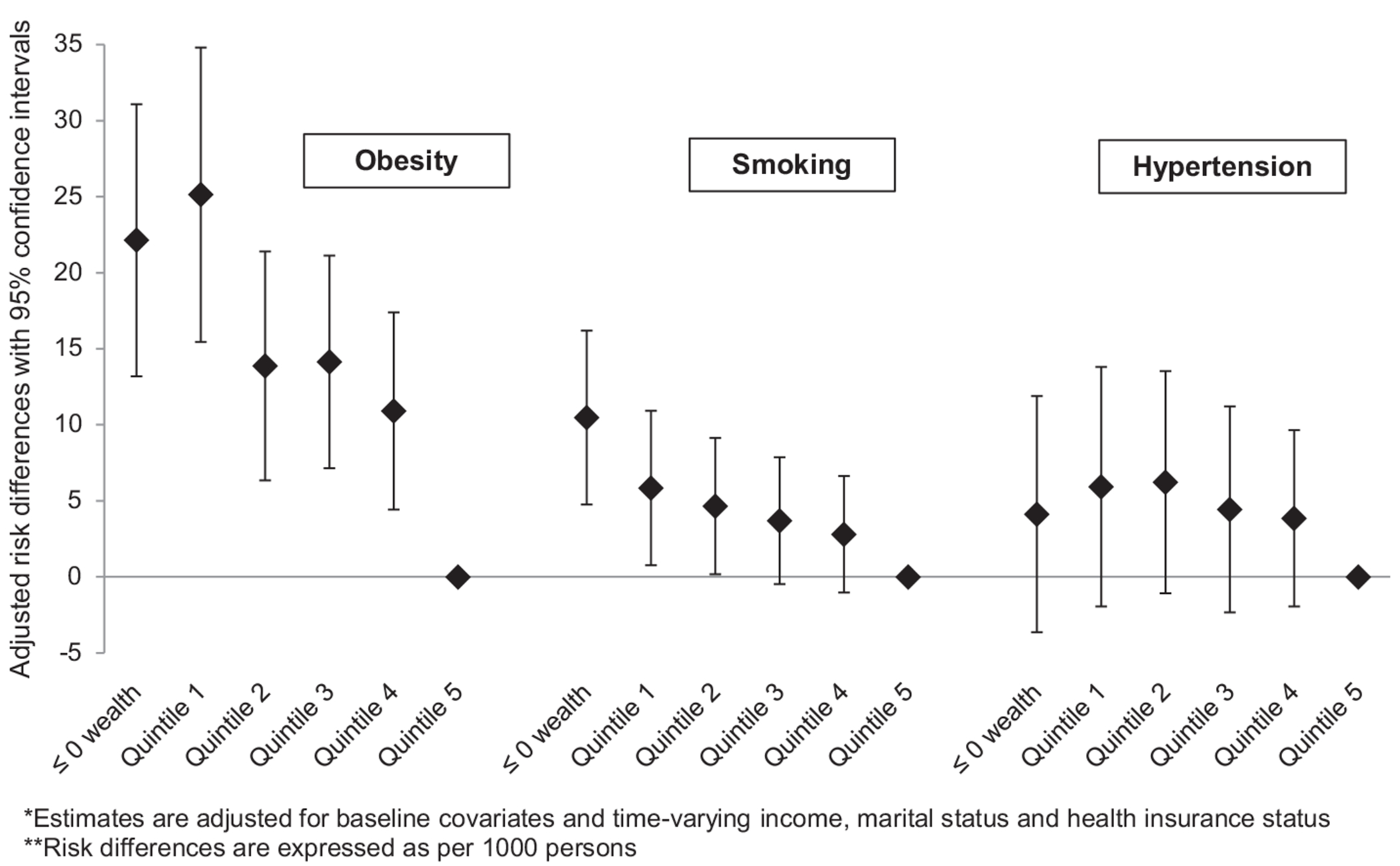
Cardiovascular disease risk factors by wealth quintile risk differences and 95% confidence intervals, PSID 1999–2005.

The estimates from the smoking model had the best precision compared to estimates from the other two models. The number of excess smokers was 10 (CI: 5, 16) for those in the less than zero wealth group, six (CI: 1,11) for the first quintile, five (CI: 0.2, 9) for the second quintile, four (CI: −0.5, 8) for the third quintile and three (CI: −1, 7) for the highest wealth group, the fourth quintile. Compared to the other models the hypertension model revealed a similar (and smaller) number of excess cases regardless of wealth quintile. The number of excess hypertensives were four (CI: −4, 12) for the least wealthy group, six for the first and second wealth quintiles (CI: −2, 14 and −1, 14 respectively), four for the third and fourth quintile (CI: −2, 11 and −2, 10 respectively).

Risk ratios and 95% confidence intervals (CI) for the effect of wealth on the three CVD risk factors are shown in Table 2. In the fully adjusted model, the risk of becoming obese was inversely related to wealth; as wealth increased the risk of obesity declined. Those with less than or equal to zero wealth and those with little wealth (quintile one) had a similar and significantly higher risk of obesity relative to the wealthiest group (quintile five), 1.80 (CI: 1.43, 2.26) and 1.89 (CI: 1.49, 2.40) respectively. Those in quintiles two and three had about a 51% (CI: 1.21, 1.88 and 1.23, 1.86 respectively) increased risk and those in quintile four a 40% (CI: 1.14, 1.71) increased risk of becoming obese compared to the wealthiest group. The confidence limit ratios suggested these estimates were relatively precise compared to estimates from other models.

Table 2.

Risk ratios and 95% confidence intervals of the association between wealth and obesity incidence, resumption or initiation of smoking and hypertension incidence, Panel Study of Income Dynamics 1999–2005.

	Obesity			Smoking			Hypertension
	Risk ratio	Lower 95% CI	Upper 95% CI	Risk ratio	Lower 95% CI	Upper 95% CI	Risk ratio	Lower 95% CI	Upper 95% CI
≤ zero wealth	1.80	1.43	2.26	2.10	1.41	3.12	1.10	0.90	1.35
Quintile 1	1.89	1.49	2.40	1.61	1.07	2.44	1.16	0.95	1.42
Quintile 2	1.51	1.21	1.88	1.50	1.01	2.21	1.17	0.97	1.41
Quintile 3	1.52	1.23	1.86	1.39	0.95	2.04	1.11	0.93	1.33
Quintile 4	1.40	1.14	1.71	1.30	0.91	1.87	1.11	0.95	1.29
Quintile 5	Referent			Referent			Referent

Note: All models adjusted for baseline covariates (sex, age, race, education, region, general health status, marital status, income and insurance status) and time-varying covariates (income, marital status and insurance status) through the IPW.

The smoking model suggested a stronger magnitude of effect for the poorest wealth group. The least wealthy had the highest risk of becoming smokers (2.10, CI: 1.41, 3.12). Those in low wealth quintiles one and two had an increased risk of becoming smokers, with RR of 1.61 (CI: 1.07, 2.44) and 1.50 (CI: 1.01, 2.21) respectively. The risk ratio for those in quintiles three was 1.39 (CI: 0.95, 2.04) and the lowest risk was among quintile four (1.30 CI: 0.91, 1.87).

The effect estimates for hypertension were more precise but of a smaller magnitude than the estimates from the other two outcomes. Among the least wealthy the model suggested that the risk of hypertension was 10% (CI: 0.90, 1.35) higher compared to the wealthiest quintile. Those in quintile one and two had about a 16% (CI for quintile one: 0.95, 1.42 and CI for quintile two: 0.97, 1.41) increased risk of developing hypertension relative to the wealthiest group, while those in quintiles three and four had an 11% increased risk of hypertension (CI: 0.93, 1.33 and 0.95, 1.29 respectively).

In order to assess the impact of time-varying confounding we compared results from the MSM to traditional models controlling for time-varying confounders. Traditional binomial models were similar in magnitude and direction to binomial MSM (see supplemental Table 2). For each estimate the confidence intervals for the traditional estimate overlapped with that of its MSM counterpart.

Discussion

This study found a strong association between wealth and obesity incidence, a moderate association between wealth and smoking initiation and a weak association between wealth and hypertension incidence. This was true on both the absolute and relative scales, where both the risk ratios and risk differences revealed similar overall patterns. Given the importance of cardiovascular disease to the US population, a closer examination of these CVD risk factors was warranted.

Other studies that examined CVD risk factors and wealth reported similar findings. Several studies on obesity found a negative association with wealth, specifically among women and whites (Demakakos et al., 2008; Fonda et al., 2004; Zagorsky, 2004a,b; Zagorsky, 2005). A German study which compared those with excess debt to those without debt found those in debt to have higher odds of obesity (Munster et al., 2009). A cross-sectional study found no association between obesity and wealth; however wealth was crudely measured (Robert & Reither, 2004). It should be noted that several of these studies were interested in the equally important question of whether poor health results in a reduction of wealth, by using wealth as the outcome and BMI as the main exposure of interest (Fonda et al., 2004; Zagorsky, 2004a,b; Zagorsky, 2005). The studies by Zagorsky conducted longitudinal analyses thus implying that obesity causes a reduction in wealth (Zagorsky, 2004a,b; Zagorsky, 2005).

The literature on smoking and wealth consisted mostly of cross-sectional studies of European or Australian populations (Laaksonen et al., 2005; Schaap et al., 2008; Siahpush et al., 2002) with one study of a US population (Kennickell, 2008). All the cross-sectional studies consistently found that the least wealthy had a higher prevalence of smoking (Kennickell, 2008; Laaksonen et al., 2005; Schaap et al., 2008; Siahpush et al., 2002). One longitudinal study interested in reverse causality found that smokers had several thousand dollars less wealth compared to non-smokers (Zagorsky, 2004a,b).

Several cross-sectional studies that looked at hypertension and wealth found stronger more significant inverse associations compared to our study (Avendano et al., 2009; Demakakos et al., 2008; Kington & Smith, 1997; Schoenbaum & Waidmann, 1997), while another found very similar results to ours (Rooks et al., 2002). Similarly, a longitudinal analysis of an elderly population in the US showed no causal link between low wealth and increased incidence of hypertension (Adams et al., 2003). It should also be noted that studies using other measures of SES such as income and education have also found a weak but positive association with hypertension (Colhoun, Hemingway, & Poulter, 1998; Pickering, 1999).

Our study had limitations. First, the use of self-reported data for some of the outcomes was not ideal. Specifically self-reported height and weight is known to underestimate the true prevalence of obesity, especially among overweight women (Gillum & Sempos, 2005; Rowland, 1990; Stommel & Schoenborn, 2009). Concerns of misclassification bias arise when classification of the outcome depends on the exposure. The less wealthy were more likely to be overweight than the wealthy, and thus were more likely to misreport their weight leading to the potential for differential misclassification. Because the less wealthy were more likely to be misclassified in their obesity status, our data showed fewer obese cases among the poor. Thus the expected direction of the misclassification for the obesity–wealth relationship in our study was towards the null.

Hypertension was most likely underreported among younger respondents who have yet to be diagnosed with hypertension, but accurately reported among older individuals who were involved in the ongoing management of the condition (Okura, Urban, Mahoney, Jacobsen, & Rodeheffer, 2004). Several studies have found that women, older and more educated individuals have less misclassification for self-reported hypertension than other groups (Colditz et al., 1986; Giles, Croft, Keenan, Lane, & Wheeler, 1995; Okura et al., 2004; Vargas, Burt, Gillum, & Pamuk, 1997). Given the relationship between wealth, age, education and health insurance status (the least wealthy tend to be younger, less educated and uninsured) we may have differential misclassification of hypertension. In light of this misclassification bias, our data would reveal fewer hypertensives among the less wealthy, thus potentially explaining the attenuated results we see for this outcome.

Misclassification of smoking status is less of a problem than for obesity or hypertension. In general researchers believe that self-reports are good indicators of actual smoking status (Caraballo, Giovino, Pechacek, & Mowery, 2001; Perez-Stable, Marin, Marin, & Benowitz, 1992; Wagenknecht, Burke, Perkins, Haley, & Friedman, 1992) because they allow us to understand the duration and severity of smoking, which biological markers (such as cotinine) do not.

In order to reduce measurement error around wealth, we also attempted additional sensitivity analysis adjusting for household size; there was little difference in the final parameter estimates comparing models that did and did not adjust for this covariate.

The exclusion of baseline cases from the analysis raises questions about selection bias, another potential source of bias in our study. Those with preexisting hypertension are more likely to be older and of lower SES. By excluding them, the effect estimate will likely be biased downward. Similarly for obesity, the exclusion of baseline cases excludes more low SES individuals which may result in underestimates of the effect. That is, a sample of healthier, wealthier individuals will create an underestimate of the effect estimate for obesity and hypertension (Flanders & Klein, 2007).

With smoking however, the picture was more complex because smoking status was a composite of a few different outcomes, each with the probability of being affected by wealth differentially. We conducted a sensitivity analysis for smoking where three separate outcomes were created for three separate subpopulations (see Supplemental Table 3). Among the non-smokers, we looked at the probability of smoking initiation. Among the current smokers we looked at the probability of quitting and among the former smokers, we looked at the probability of resuming smoking. Each of these outcomes was fit using a logistic MSM (because outcomes were rare). Results from these models all went in the expected direction. Although the number of persons who initiated smoking was small, there was an elevated odds of smoking initiation among the least wealthy individuals, which declined as wealth increased. The smoking cessation model showed that the least wealthy were less likely to quit smoking, while the wealthier quintiles were more likely to do so. Lastly, in the smoking resumption model, the least wealthy were more likely to resume smoking while the wealthier quintiles were more likely to remain non-smokers. The results of these models provided some assurance that selection bias was not severely affecting the estimates in the overall smoking model. It should be noted that in addition to modeling incidence, we also modeled prevalence for each of the outcomes. Results were similar, however, incidence models produces estimates of larger magnitude.

A final limitation of our study is that we do not incorporate any area-level wealth measures in our analysis. Area-level measures of wealth are difficult to obtain and measures that do exist, such as home-values, do not sufficiently capture a community’s true level of wealth as they do not generally account for mortgage debt. Other area-level measures are aggregated at the state or county level resulting in limited variation.

There were several strengths to our study. First, wealth alone is rarely used as a measure of SES in health research; our paper contributes to the literature as one of the few papers to assess the main effects of wealth on CVD risk factors. Furthermore, by using data from the PSID, we were assured that wealth was measured in a rigorous and comprehensive fashion (Curtin et al., 1989). Secondly, the presentation of both absolute and relative measures of effect provides a more interpretable result than previous studies. In addition, the longitudinal nature of the PSID allowed us to explore the question of wealth and health over a 6 year period. Most studies of wealth and health to date have used cross-sectional data. A related advantage was our use of marginal structural models as the analytic technique to answer the study question. This was the first study of wealth and health outcomes to employ such methods. After satisfying several important assumptions, such as the absence of unmeasured confounding, MSM can have a causal interpretation even in the presence of time-varying confounding. Although some of the assumptions of MSM are difficult to meet, we believe this study produced improved estimates relative to past studies (Levine, 2009). A randomized controlled trial which randomly assigns wealth to each individual at baseline and then again after 2 years of follow-up (as our study does) and waits for the development of one of the CVD risk factors would yield an estimate with a causal interpretation. Since wealth is not easily randomizable, the consistency assumption is suspect; therefore, the true causal estimates of the relationship between wealth and health may not equal the estimates presented in our study, regardless of our improved methodology.

As noted earlier, the results we obtained from MSM were similar to those from traditional models. This indicates that there was not a substantial amount of time-varying confounding in our study. We hypothesized that income would be the strongest time-varying confounder. However, given our study’s short time interval, income trajectories remained relatively stable during this period (see Supplemental Fig. 1 for a graph of average inflation-adjusted income over the study period); thus it is understandable that income was not a strong time-varying confounder in these data.

An additional time-varying confounder of potential importance is health status. We conducted a sensitivity analysis where lagged general health status was included as a time-varying covariate. Results from these models (Supplemental Tables 4 and 5) generally showed a stronger magnitude of effect for obesity and hypertension. These results are expected as confounding by health status is likely to be stronger with conditions that take a longer time to develop.

There are many potential mechanisms through which low wealth results in poor health outcomes. Poor physical and social environments can encourage health-damaging exposures (Adler & Rehkopf, 2008). For example, the lack of economic resources associated with having little wealth may limit an individual’s access to health care, quality housing and nutritious foods among other things. A lack of economic and social resources can also result in insufficient investment in “human, physical, social and health infrastructure” which may be detrimental to the health of populations (Lynch, Smith, Kaplan, & House, 2000). Assuming that less wealthy individuals live in less wealthy communities, insufficient infrastructure may take the form of fewer or less convenient public transportation options, a lack of parks and unsafe streets, and more liquor and convenient stores. These deficiencies can then lead to increased isolation, a more sedentary lifestyle and poor diets, which directly result in higher rates of smoking and obesity among less wealthy individuals (Chaix, 2009; Diez Roux, 2003). Other research has found that low SES individuals may have less social support, higher job strain and less job control. All these factors have been associated with higher rates of smoking and obesity (Taylor, Repetti, & Seeman, 1997).

Chronic stress may underlie many of these health-damaging exposures (Adler & Rehkopf, 2008). Since wealth is a stockpile of financial resources a lack of wealth (which translates into the absence of a safety net) is ostensibly a cause for long-term financial stress. It has been hypothesized that chronic stress and other psychosocial factors trigger a series of biological events, through central nervous system activation of autonomic, neuroendocrine and immune responses (Steptoe & Marmot, 2002). These biological pathways may be especially germane to hypertension and other cardiovascular functions (Steptoe et al., 2002). The choice of CVD risk factors as outcomes for this study was further underscored in light of the potential mechanisms discussed above.

Although wealth may be more difficult to measure than other SES variables, both its empirical performance and its theoretical relevance make it an important factor that should be considered by more health researchers. In addition, asset building programs focusing on the poor and middle class have shown modest success in helping families build wealth (McKernan & Sherraden, 2008). Thus, not only is wealth a useful empirical and theoretical construct, it is also amenable to policy interventions that could have long-term benefits for improving the health of the poor.

References

- Adams P, Hurd MD, McFadden D, Merrill A, & Ribeiro T (2003). Healthy, wealthy, and wise? Tests for direct causal paths between health and socioeconomic status. Journal of Econometrics, 112(1), 3–56. [Google Scholar]
- Adler NE, & Rehkopf DH (2008). U.S. disparities in health: descriptions, causes, and mechanisms. Annual Review of Public Health, 29, 235–252. [DOI] [PubMed] [Google Scholar]
- Angeles G, Guilkey DK, & Mroz TA (2005). The impact of community-level variables on individual-level outcomes: theoretical results and applications. Sociological Methods & Research, 34(1), 76–121. [Google Scholar]
- An overview of the panel study of income dynamics. (2009). http://psidonline.isr.umich.edu/Guide/Overview.html Retrieved October 13. 2010.
- Avendano M, Glymour MM, Banks J, & Mackenbach JP (2009). Health disadvantage in US adults aged 50 to 74 years: a comparison of the health of rich and poor Americans with that of Europeans. American Journal of Public Health, 99(3), 540–548. [DOI] [PMC free article] [PubMed] [Google Scholar]
- Braveman PA, Cubbin C, Egerter S, Chideya S, Marchi KS, Metzler M, et al. (2005). Socioeconomic status in health research: one size does not fit all. JAMA: The Journal of the American Medical Association, 294(22), 2879–2888. [DOI] [PubMed] [Google Scholar]
- Cagney KA, & Lauderdale DS (2002). Education, wealth, and cognitive function in later life. The Journals of Gerontology. Series B, Psychological Sciences and Social Sciences, 57(2), P163–P172. [DOI] [PubMed] [Google Scholar]
- Caraballo RS, Giovino GA, Pechacek TF, & Mowery PD (2001). Factors associated with discrepancies between self-reports on cigarette smoking and measured serum cotinine levels among persons aged 17 years or older: third national health and nutrition examination survey, 1988–1994. American Journal of Epidemiology, 153(8), 807–814. [DOI] [PubMed] [Google Scholar]
- Chaix B (2009). Geographic life environments and coronary heart disease: a literature review, theoretical contributions, methodological updates, and a research agenda. Annual Review of Public Health, 30, 81–105. [DOI] [PubMed] [Google Scholar]
- Colditz GA, Martin P, Stampfer MJ, Willett WC, Sampson L, Rosner B, et al. (1986). Validation of questionnaire information on risk factors and disease outcomes in a prospective cohort study of women. American Journal of Epidemiology, 123(5), 894–900. [DOI] [PubMed] [Google Scholar]
- Cole SR, & Hernan MA (2008). Constructing inverse probability weights for marginal structural models. American Journal of Epidemiology, 168(6), 656–664. [DOI] [PMC free article] [PubMed] [Google Scholar]
- Colhoun HM, Hemingway H, & Poulter NR (1998). Socio-economic status and blood pressure: an overview analysis. Journal of Human Hypertension, 12(2), 91–110. [DOI] [PubMed] [Google Scholar]
- Curtin R, Juster FT, & Morgan J (1989). Survey estimates of wealth: an assessment of quality. In Lipsey RE, & Tice HS (Eds.), The measurement of saving, investment, and wealth (pp. 473–548). Chicago, IL: University of Chicago Press. [Google Scholar]
- Demakakos P, Nazroo J, Breeze E, & Marmot M (2008). Socioeconomic status and health: the role of subjective social status. Social Science & Medicine (1982), 67(2), 330–340. [DOI] [PMC free article] [PubMed] [Google Scholar]
- Diez Roux AV (2003). Residential environments and cardiovascular risk. Journal of Urban Health: Bulletin of the New York Academy of Medicine, 80(4), 569–589. [DOI] [PMC free article] [PubMed] [Google Scholar]
- Flanders WD, & Klein M (2007). Properties of 2 counterfactual effect definitions of a point exposure. Epidemiology, 18(4), 453–460, (Cambridge, Mass). [DOI] [PubMed] [Google Scholar]
- Fonda SJ, Fultz NH, Jenkins KR, Wheeler LM, & Wray LA (2004). Relationship of body mass and net worth for retirement-aged men and women. Research on Aging, 26(1), 153. [Google Scholar]
- Giles WH, Croft JB, Keenan NL, Lane MJ, & Wheeler FC (1995). The validity of self-reported hypertension and correlates of hypertension awareness among blacks and whites within the stroke belt. American Journal of Preventive Medicine, 11(3), 163–169. [PubMed] [Google Scholar]
- Gillum RF, & Sempos CT (2005). Ethnic variation in validity of classification of overweight and obesity using self-reported weight and height in American women and men: the third national health and nutrition examination survey. Nutrition Journal, 4, 27. [DOI] [PMC free article] [PubMed] [Google Scholar]
- Hernan MA, Brumback B, & Robins JM (2000). Marginal structural models to estimate the causal effect of zidovudine on the survival of HIV-positive men. Epidemiology (Cambridge, Mass), 11(5), 561–570. [DOI] [PubMed] [Google Scholar]
- Keister LA (2000). Wealth in America: Trends in wealth inequality. Cambridge, U.K: Cambridge University Press. [Google Scholar]
- Kennickell AB (2008). What is the difference? Evidence on the distribution of wealth, health, life expectancy, and health insurance coverage. Statistics in Medicine, 27(20), 3927–3940. [DOI] [PubMed] [Google Scholar]
- Kington RS, & Smith JP (1997). Socioeconomic status and racial and ethnic differences in functional status associated with chronic diseases. American Journal of Public Health, 87(5), 805–810. [DOI] [PMC free article] [PubMed] [Google Scholar]
- Laaksonen M, Rahkonen O, Karvonen S, & Lahelma E (2005). Socioeconomic status and smoking: analysing inequalities with multiple indicators. European Journal of Public Health, 15(3), 262–269. [DOI] [PubMed] [Google Scholar]
- Levine B (2009). Re: Bringing causal models into the mainstream (letter). Epidemiology, 20(3), 431. [DOI] [PubMed] [Google Scholar]
- Lynch JW, Smith GD, Kaplan GA, & House JS (2000). Income inequality and mortality: importance to health of individual income, psychosocial environment, or material conditions. British Medical Journal (Clinical Research Ed.), 320 (7243), 1200–1204. [DOI] [PMC free article] [PubMed] [Google Scholar]
- McKernan SM, & Sherraden M (2008). Asset building and low-income families. Urban Institute Press. [Google Scholar]
- Menchik PL (1993). Economic status as a determinant of mortality among black and white older men: does poverty kill? Population Studies, 47(3), 427–436. [Google Scholar]
- Miglioretti DL, & Heagerty PJ (2007). Marginal modeling of non nested multilevel data using standard software. American Journal of Epidemiology, 165(4), 453–463. [DOI] [PubMed] [Google Scholar]
- Munster E, Ruger H, Ochsmann E, Letzel S, & Toschke AM (2009). Over-indebtedness as a marker of socioeconomic status and its association with obesity: a cross-sectional study. BMC Public Health, 9, 286. [DOI] [PMC free article] [PubMed] [Google Scholar]
- Oehlert GW (1992). A note on the delta method. American Statistician 27–29. [Google Scholar]
- Okura Y, Urban LH, Mahoney DW, Jacobsen SJ, & Rodeheffer RJ (2004). Agreement between self-report questionnaires and medical record data was substantial for diabetes, hypertension, myocardial infarction and stroke but not for heart failure. Journal of Clinical Epidemiology, 57(10), 1096–1103. [DOI] [PubMed] [Google Scholar]
- Perez-Stable EJ, Marin G, Marin BV, & Benowitz NL (1992). Misclassification of smoking status by self-reported cigarette consumption. The American Review of Respiratory Disease, 145(1), 53–57. [DOI] [PubMed] [Google Scholar]
- Pickering T (1999). Cardiovascular pathways: socioeconomic status and stress effects on hypertension and cardiovascular function. Annals of the New York Academy of Sciences, 896, 262–277. [DOI] [PubMed] [Google Scholar]
- Pollack CE, Chideya S, Cubbin C, Williams B, Dekker M, & Braveman P (2007). Should health studies measure wealth? A systematic review. American Journal of Preventive Medicine, 33(3), 250–264. [DOI] [PubMed] [Google Scholar]
- Robert SA, & Reither EN (2004). A multilevel analysis of race, community disadvantage, and body mass index among adults in the US. Social Science & Medicine (1982), 59(12), 2421–2434. [DOI] [PubMed] [Google Scholar]
- Robins JM, Hernan MA, & Brumback B (2000). Marginal structural models and causal inference in epidemiology. Epidemiology, 11(5), 550–560, (Cambridge, Mass). [DOI] [PubMed] [Google Scholar]
- Rooks RN, Simonsick EM, Miles T, Newman A, Kritchevsky SB, Schulz R, et al. (2002). The association of race and socioeconomic status with cardiovascular disease indicators among older adults in the health, aging, and body composition study. The Journals of Gerontology. Series B, Psychological Sciences and Social Sciences, 57(4), S247–S256. [DOI] [PubMed] [Google Scholar]
- Rowland ML (1990). Self-reported weight and height. The American Journal of Clinical Nutrition, 52(6), 1125–1133. [DOI] [PubMed] [Google Scholar]
- Schaap MM, van Agt HM, & Kunst AE (2008). Identification of socioeconomic groups at increased risk for smoking in European countries: looking beyond educational level. Nicotine & Tobacco Research: Official Journal of the Society for Research on Nicotine and Tobacco, 10(2), 359–369. [DOI] [PubMed] [Google Scholar]
- Schoenbaum M, & Waidmann T (1997). Race, socioeconomic status, and health: accounting for race differences in health. The Journals of Gerontology. Series B, Psychological Sciences and Social Sciences, 52(Spec No), 61–73. [DOI] [PubMed] [Google Scholar]
- Shapiro TM, & Wolff EN (2001). Assets for the poor: The benefits of spreading asset ownership. New York: Russell Sage Foundation. [Google Scholar]
- Siahpush M, Borland R, & Scollo M (2002). Prevalence and socio-economic correlates of smoking among lone mothers in Australia. Australian and New Zealand Journal of Public Health, 26(2), 132–135. [DOI] [PubMed] [Google Scholar]
- Smith JP, & Kington R (1997). Race, socioeconomic status, and health in late life. In Martin L, & Solbo B (Eds.), Racial and ethnic differences in the health of older Americans (pp. 106–162). Washington, DC: Natl Academy Pr. [Google Scholar]
- Spiegelman D, & Hertzmark E (2005). Easy SAS calculations for risk or prevalence ratios and differences. American Journal of Epidemiology, 162(3), 199–200. [DOI] [PubMed] [Google Scholar]
- StataCorp L (2007). Stata statistical software. Release 10. [Google Scholar]
- Steptoe A, Feldman PJ, Kunz S, Owen N, Willemsen G, & Marmot M (2002). Stress responsivity and socioeconomic status. A mechanism for increased cardiovascular disease risk? European Heart Journal, 23(22), 1757. [DOI] [PubMed] [Google Scholar]
- Steptoe A, & Marmot M (2002). The role of psychobiological pathways in socioeconomic inequalities in cardiovascular disease risk. European Heart Journal, 23 (1), 13–25. [DOI] [PubMed] [Google Scholar]
- Stommel M, & Schoenborn CA (2009). Accuracy and usefulness of BMI measures based on self-reported weight and height: findings from the NHANES & NHIS 2001–2006. BMC Public Health, 9, 421. [DOI] [PMC free article] [PubMed] [Google Scholar]
- Taylor SE, Repetti RL, & Seeman T (1997). Health psychology: what is an unhealthy environment and how does it get under the skin? Annual Review of Psychology, 48, 411–447. [DOI] [PubMed] [Google Scholar]
- Vargas CM, Burt VL, Gillum RF, & Pamuk ER (1997). Validity of self-reported hypertension in the national health and nutrition examination survey III, 1988–1991. Preventive Medicine, 26(5 Pt 1), 678–685. [DOI] [PubMed] [Google Scholar]
- Wagenknecht LE, Burke GL, Perkins LL, Haley NJ, & Friedman GD (1992). Misclassification of smoking status in the CARDIA study: a comparison of self-report with serum cotinine levels. American Journal of Public Health, 82(1), 33–36. [DOI] [PMC free article] [PubMed] [Google Scholar]
- Wilkinson RG (1999). Health, hierarchy, and social anxiety. Annals of the New York Academy of Sciences, 896, 48–63. [DOI] [PubMed] [Google Scholar]
- Wolff E (1995). Top heavy: A study of the increasing inequality of wealth in America. New York, NY: Twentieth Century Fund. [Google Scholar]
- Zagorsky JL (2004a). Is obesity as dangerous to your wealth as to your health? Research on Aging, 26(1), 130. [Google Scholar]
- Zagorsky JL (2004b). The wealth effects of smoking. Tobacco Control, 13(4), 370–374. [DOI] [PMC free article] [PubMed] [Google Scholar]
- Zagorsky JL (2005). Health and wealth. The late-20th century obesity epidemic in the U.S. Economics and Human Biology, 3(2), 296–313. [DOI] [PubMed] [Google Scholar]
Associated Data
This section collects any data citations, data availability statements, or supplementary materials included in this article.