



Abstract
Contemporary pose estimation methods enable precise measurements of behavior via supervised deep learning with hand-labeled video frames. Although effective in many cases, the supervised approach requires extensive labeling and often produces outputs that are unreliable for downstream analyses. Here, we introduce ‘Lightning Pose’, an efficient pose estimation package with three algorithmic contributions. First, in addition to training on a few labeled video frames, we use many unlabeled videos and penalize the network whenever its predictions violate motion continuity, multiple-view geometry and posture plausibility (semi-supervised learning). Second, we introduce a network architecture that resolves occlusions by predicting pose on any given frame using surrounding unlabeled frames. Third, we refine the pose predictions post hoc by combining ensembling and Kalman smoothing. Together, these components render pose trajectories more accurate and scientifically usable. We released a cloud application that allows users to label data, train networks and process new videos directly from the browser.
Behavior is a window into the processes that underlie animal intelligence, ranging from early sensory processing to complex social interaction1. Methods for automatically quantifying behavior from video2–4 have opened the door to high-throughput experiments that compare animal behavior across pharmacological5 and disease6 conditions.
Pose estimation methods based on fully supervised deep learning have emerged as a workhorse for behavioral quantification7–11. This technology reduces high-dimensional videos of behaving animals to low-dimensional time series of their poses, defined in terms of a small number of user-selected keypoints per video frame. Three steps are required to accomplish this feat. Users first create a training dataset by manually labeling poses on a subset of video frames; typically, hundreds or thousands of frames are labeled to obtain reliable pose estimates. A neural network is then trained to predict poses that match user labels. Finally, the network processes a new video to predict a pose for each frame separately. Each predicted keypoint is accompanied by a confidence score, and low-confidence predictions are typically dropped. This process of labeling–training–prediction can be iterated until performance is satisfactory. The tracked poses are used in downstream analyses including quantifying predefined behavioral features (for example, gait features such as stride length, or social features such as distance between subjects), estimation of neural encoding and decoding models, classification of behaviors into discrete ‘syllables’ and closed-loop experiments12–17.
Although the supervised paradigm is effective in many cases, a number of roadblocks remain. To start, image labeling can be laborious, especially when handling complicated skeletons across multiple views. Even with large, labeled datasets, trained networks often produce ‘glitchy’ predictions that require further manipulation before downstream analyses18,19, and struggle to generalize to subjects and sessions outside their training data. Even networks that achieve low error rates on labeled test frames can still produce error frames that hinder downstream scientific tasks. Manually identifying these error frames is like finding a needle in a haystack20: errors persist for a few frames at a time, whereas behavioral videos can be hours long. Automatic approaches—currently limited to filtering low-confidence predictions and temporal discontinuities—can miss scientifically critical errors.
To improve the robustness and usability of animal pose estimation, we present Lightning Pose, a solution at three levels: modeling, software and a cloud-based application.
First, we leverage semi-supervised learning, which involves training networks on both labeled frames and unlabeled videos, and is known to improve generalization and data efficiency21. On unlabeled videos, the networks are trained to minimize a number of unsupervised losses that encode our prior beliefs about moving bodies: poses should evolve smoothly in time, be physically plausible, and be localized consistently when seen from multiple views. In addition, we leverage unlabeled frames in a temporal context network (TCN) architecture, which instead of processing a single frame at a time, processes each frame with its neighboring (unlabeled) frames. Our resulting models outperform their purely supervised counterparts across datasets, providing more reliable predictions for downstream analyses. We further improve our networks’ predictions using a general Bayesian post-processing approach, which we coin the ensemble Kalman smoother (EKS): we aggregate (‘ensemble’) the predictions of multiple networks—which is known to improve their accuracy and robustness22,23—and model those aggregated predictions with a spatially constrained Kalman smoother that takes their collective uncertainty into account.
We implemented these tools in a deep learning software package that capitalizes on recent advances in the deep learning ecosystem. We name our package Lightning Pose, as it is based on the PyTorch Lightning deep learning library24. Unlike most existing packages, Lightning Pose is video centric and built for manipulating large videos directly on the graphics processing unit (GPU), to support our semi-supervised training.
Finally, we developed a no-install cloud application that is accessed from the browser and enables users to annotate data, train networks and diagnose performance without requiring programming skills or specialized hardware.
Results
Supervised pose estimation and its limitations
The leading packages for animal pose estimation—DeepLabCut7, SLEAP8, DeepPoseKit9 and others—differ in architectures and implementation but all perform supervised heat map regression on a frame-by-frame basis (Fig. 1a). A standard model is composed of a ‘backbone’ that extracts features for each frame (for example, a ResNet-50 network) and a ‘head’ that uses these features to predict body part location heat maps. Networks are trained to match their outputs to manual labels.
Fig. 1|. Fully supervised pose estimation often outputs unstable predictions and requires many labels to generalize to new animals.
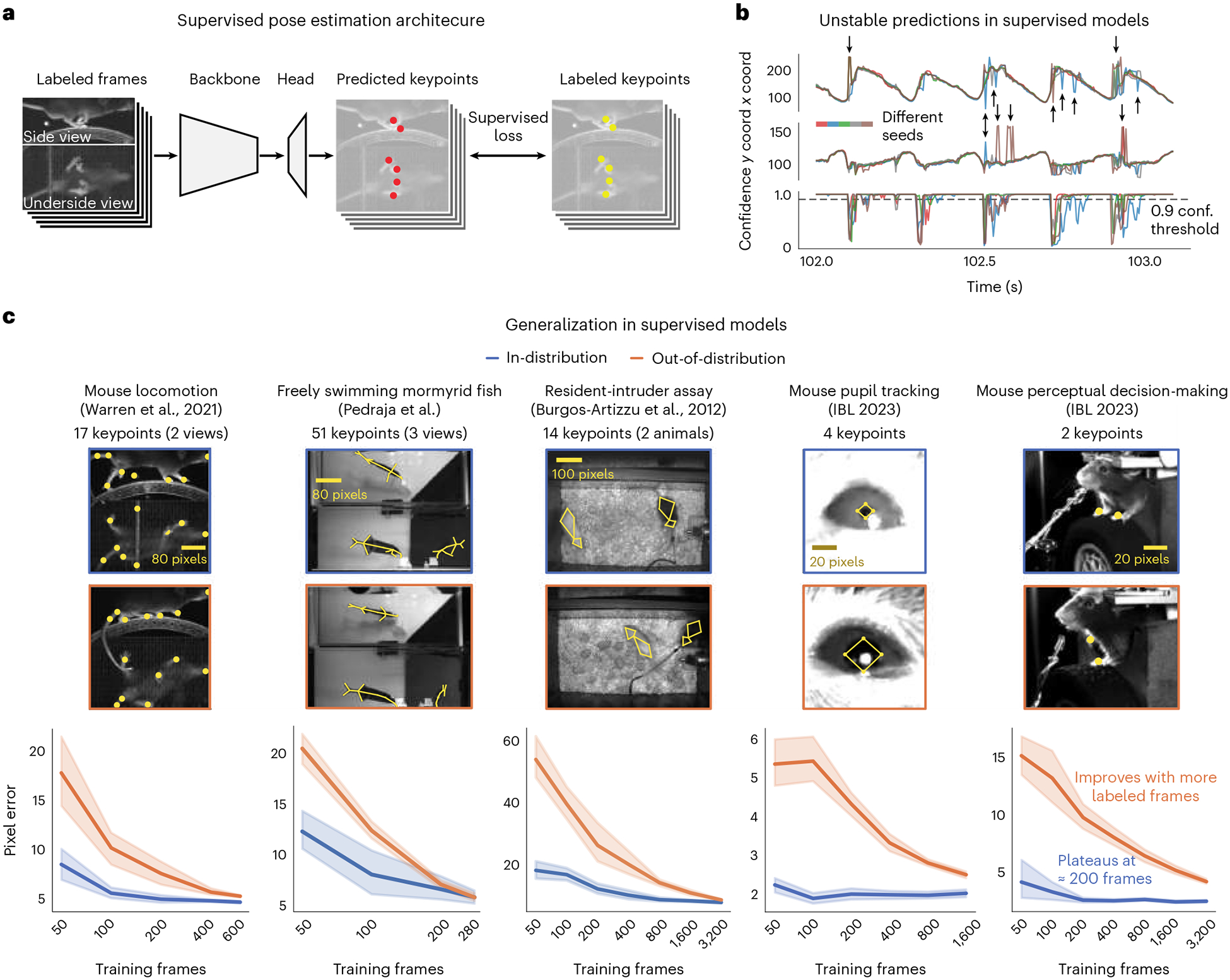
a, Diagram of a typical pose estimation model trained with supervised learning, illustrated using the mirror-mouse dataset. A dataset is created by labeling keypoints on a subset of video frames. A convolutional neural network, consisting of a ‘backbone’ and a prediction ‘head’, takes in a batch of frames as inputs, and predicts a set of keypoints for each frame. It is trained to minimize the distance from the labeled keypoints. b, Predictions from five supervised DeepLabCut networks (trained with 631 labeled frames on the mirror-mouse dataset), for the left front paw position (top view) during 1 s of running behavior (Supplementary Video 1). Top, -coordinate; middle, -coordinate; bottom, confidence, applying a standard 0.9 threshold indicated by the dashed line. Black arrows indicate example time points where there is disagreement among the network predictions. c, Top row shows five example datasets. Each blue image is an example taken from the InD test set, which contains new images of animals that were seen in the training set. The orange images are test examples from unseen animals altogether, which we call the OOD test set. Bottom row shows data efficiency curves, measuring test-set pixel error as a function of the training set size. InD pixel error is shown in blue and OOD in orange. Line plots show the mean pixel error across all keypoints and frames ± s.e. over random subsets of InD training data.
Even when trained with many labeled frames, pose estimation network outputs may still be erroneous. We highlight this point using the ‘mirror-mouse’ dataset, which features a head-fixed mouse running on a treadmill and performing a sensory-guided locomotion task14. Using a camera and a bottom mirror, the mouse’s side and underside are observed simultaneously, recorded at 250 frames per second. Seventeen body parts are tracked, including all four paws in both views. We trained five DeepLabCut networks on 631 labeled frames (for each network, we used a different random seed to split the labeled frames into train and test sets).
We analyzed the time series of the estimated left hind paw position during 1 s of running behavior for each of the five networks (Fig. 1b). Each time series exhibited the expected periodic pattern (due to the running gait), but included numerous ‘glitches’, some of which are undetected by the networks’ confidence. This collection of five networks—also known as a ‘deep ensemble’22—outputs variable predictions on many frames, especially in challenging moments of ambiguity or occlusion (Supplementary Video 1). We will later use this ensemble variance as a proxy for keypoint ‘difficulty’.
Supervised networks need more labeled data to generalize
It is standard to train a pose estimator using a representative sample of subjects, evaluate performance on held-out examples from that sample (‘in-distribution’ test set, henceforth InD), then deploy the network for incoming data. The incoming data may include new subjects, seen from slightly different angles or lighting conditions (‘out-of-distribution’ test set, henceforth OOD). Differences between the InD and OOD test sets are termed ‘OOD shifts’25,26.
We analyzed five datasets: ‘mirror-mouse’14, a freely swimming mormyrid fish imaged with a single camera and two mirrors (for three views in total; ‘mirror-fish,’ Supplementary Fig. 1), a resident-intruder assay27,28 (‘CRIM13;’ top-down view), paw tracking in a head-fixed mouse29 (‘IBL-paw;’ side view), and a crop of the pupil area in IBL-paw (‘IBL-pupil’). We split each labeled dataset into two cohorts of subjects, InD and OOD (Supplementary Table 1).
We trained supervised networks that use a pretrained ResNet-50 backbone, similar to DeepLabCut, on InD data with an increasing number of labeled frames. Ten networks were trained per condition, each on a different random subset of InD data. We evaluated the networks’ performance on held-out InD and OOD labeled examples. We first replicated the observation that InD test-set error plateaus starting from ~200 labeled frames16 (Fig. 1c). From looking at this curve in isolation, it could be inferred that additional manual annotation is unnecessary. However, the OOD error curve keeps steeply declining as more labels are added. This larger label requirement is consistent with recent work showing that ~50,000 labeled frames are needed to robustly track ape poses30, and that mouse face tracking networks need to be explicitly fine-tuned on labeled OOD data to achieve good performance31.
To address these limitations, we developed the Lightning Pose framework, comprising two components: semi-supervised learning and a TCN architecture.
Semi-supervised learning via spatiotemporal constraints
Most animal pose estimation algorithms treat body parts as independent in time and space. Moreover, they do not train on the vast amounts of available unlabeled videos. These two observations offer an opportunity for semi-supervised learning21. We thus train a network on both labeled frames (supervised) and large volumes of unlabeled videos (unsupervised; Fig. 2a). For unlabeled videos, the network outputs a time series of pose predictions. These predictions are subjected to a set of spatiotemporal constraints, and severe violations of these constraints incur penalties (with a controllable threshold parameter ). The unsupervised losses are applied only during training and hence do not affect video prediction speeds.
Fig. 2 |. Lightning Pose exploits unlabeled data in pose estimation model training.

a, Diagram of the semi-supervised model that contains supervised (top row) and unsupervised (bottom row) components. b, Temporal difference loss. Top left: illustration of a jump discontinuity. Top right: loss landscape for frame t given the prediction at (white diamond), for the left front paw (top view). The dark blue circle corresponds to the maximum allowed jump, below which the loss is set to zero. Bottom left: correlation between temporal difference loss and pixel error on labeled test frames. c, Multi-view PCA loss. Top left: illustration of a 3D keypoint detected on the imaging plane of two cameras. Top right: loss landscape for the left front paw (top view; white diamond) given its predicted location on the bottom view. The blue band of low loss values is an ‘epipolar line’ on which the top-view paw could be located. Bottom left: correlation between multi-view PCA loss and pixel error. Bottom right: cumulative variance explained for single body part labels across all views versus the fraction of principal components (PCs) kept on multi-view datasets. d, Pose PCA loss. Top left: illustration of plausible and implausible poses. Top right: loss landscape for the left front paw (top view; white diamond) given all other keypoints, which is minimized around the paw’s actual position. Bottom left: correlation between Pose PCA loss and pixel error. Bottom right: cumulative variance explained for pose labels versus fraction of PCs kept. e, The TCN processes each labeled frame with its adjacent unlabeled frames, using a bidirectional CRNN. It forms two sets of location heat map predictions, one using single-frame information and another using temporal context.
Temporal difference loss
The first spatiotemporal constraint we introduce is also one held by 4-month-old infants: objects should move continuously32 and not jump too far between video frames. We define the temporal difference loss for each body part as the Euclidean distance between consecutive predictions in pixels. Similar losses have been used to detect outlier predictions post hoc14,31, whereas our goal is to incorporate these losses directly into network training33.
The threshold ϵ indicates the maximum allowed jump, forming a ball of zero-loss values around the previous prediction; it should be set depending on the frame rate, frame size, the camera’s distance from the subject, and how quickly or jerkily the subject moves (Fig. 2b).
If our losses are indeed viable proxies for pose prediction errors, they should be correlated with pixel errors in labeled test frames. We analyzed the predictions of a supervised model trained with 75 labeled frames, and found a mild correlation between the temporal difference loss and pixel errors (log-linear regression: Pearson , 95% confidence interval (CI) = [0.20, 0.32]; Fig. 2b). The mild correlation here is expected: errors that persist across multiple frames will exhibit a low temporal difference loss; in periods of fast motion, the temporal difference loss will be high even when keypoint predictions are accurate. As a comparison, confidence is a more reliable predictor of pixel error Pearson , 95% CI = [−0.59, −0.49]).
Multi-view PCA loss
The common pipeline for three-dimensional (3D) tracking in neuroscience includes three steps: (1) calibrating multiple cameras using a physical calibration board, (2) training a network to estimate a 2D pose independently in each camera, and (3) triangulating the 2D poses into a 3D pose using standard computer vision techniques18,34. The common pipeline has two limitations. First, camera calibration is brittle (especially for small experimental setups) and adds experimental complexity. Second, network training is blind to the dependencies between the views.
The ‘multi-view PCA’ loss constrains the predictions for unlabeled videos to be consistent across views35,36, while bypassing the need for camera calibration. Each multi-view prediction contains width–height pixel coordinates for a single keypoint across all views. We use principal component analysis (PCA)—a linear method—to compress each multi-view prediction into three dimensions, and then expand it back into the original pixel coordinates (henceforth, ‘PCA reconstruction’). We define the multi-view PCA loss as the pixel error between the original versus the PCA-reconstructed prediction, averaged across keypoints and views. The multi-view PCA loss should approach zero when the predictions are consistent across views and when nonlinear camera distortions are negligible (Fig. 2c). Substantial distortions may be introduced by the lens or a water medium; this simple linear approach will not be robust in these cases. Practically, however, in both the mirror-mouse (two views) and mirror-fish (three views) datasets, distortions were minimized by placing the camera far from the subject (~1.1 m and ~1.7 m, respectively). In both cases, three PCA dimensions explained >99.9% of the multi-view ground truth label variance (Fig. 2c).
For a single frame of the mirror-mouse dataset, we computed the loss landscape for the left front paw on the top view, given its position in the bottom view. According to multiple-view geometry, a point identified in one camera constrains the corresponding point in a second camera to a specific line, known as the ‘epipolar line’37. Indeed, the loss landscape exhibits a line of low loss values that intersects with the paw’s true location (Fig. 2c). The multi-view loss is strongly correlated with pixel error in a test set of labeled OOD frames (Pearson , 95% CI = [0.87, 0.90]), much more so than the temporal difference loss or confidence, motivating its use both as a post hoc quality metric and as a penalty during training.
Pose PCA loss
Not all body configurations are feasible, and of those that are feasible, many are unlikely. Even diligent yoga practitioners will find their head next to their foot only on rare occasions (Fig. 2d). The Pose PCA loss constrains the predicted pose to lie on a low-dimensional subspace of feasible and likely body configurations. It is defined as the pixel error between an original pose prediction and its reconstruction after low-dimensional compression.
This loss is inspired by the success of low-dimensional models in capturing biological movement38, ranging from worm locomotion39 to human hand grasping40. We similarly find that across four of our datasets, 99% of the pose variance can be explained with far fewer dimensions than the number of pose coordinates (Fig. 2d)—mirror-mouse: 14/28 components; mirror-fish: 8/40; CRIM13: 8/28; IBL-pupil 3/8 (IBL-paw only contains four dimensions). The effective pose dimensionality depends on the complexity of behavior, the keypoints selected for labeling and the quality of the labeling. Pose dimensionality will be lower for sets of spatially correlated keypoints, and higher in the presence of labeling errors that reduce these correlations.
Using an example from the mirror-mouse dataset, we computed the PCA loss landscape for the left hind paw given the location of all the other body parts, finding that the loss strongly favors predictions in the vicinity of the true paw location (Fig. 2d). Across all labeled OOD frames, Pose PCA loss closely tracks ground truth pixel error (Fig. 2d; Pearson , 95% CI = [0.90, 0.92]). The Pose PCA loss might erroneously penalize valid postures that are not represented in the labeled dataset. To test the prevalence of this issue, we took DeepLabCut models trained with abundant labels and computed the Pose PCA loss on held-out videos. We collected 100 frames with the largest Pose PCA loss per dataset. Manual labeling revealed that 85/100 (mirror-mouse; Supplementary Video 2), 87/100 (mirror-fish; Supplementary Video 3) and 100/100 (CRIM13; Supplementary Video 4) of the frames include true errors, indicating that in most cases, large Pose PCA losses correspond to pose estimation errors, rather than unseen rare poses.
TCN
When labeling frames that contain occlusions or ambiguities, practitioners often scroll the video to help ‘fill in the gaps’. This useful temporal context is not provided to standard architectures that process one frame at a time.
Therefore, we developed a TCN (Fig. 2e), which uses a frame sequence to predict the location heat maps for the middle (that is, ) frame. As in the standard architecture, the TCN starts by pushing each image through a backbone that extracts useful features. Then, instead of predicting the pose directly from each of these individual features, a bidirectional convolutional recurrent neural network (CRNN) is applied to the time series of features; the CRNN outputs a prediction only for the middle frame. The CRNN is lightweight compared to the backbone, and we only apply the backbone once per frame; therefore, the TCN runtime scales linearly with the number of total context frames. We have found that a context window of five frames (that is, ) provides an effective balance between speed and accuracy and have used this value throughout the paper. The outputs of the TCN and the single-frame model tend to match on fully visible keypoints, and differ on occluded or ambiguous keypoints.
Spatiotemporal losses enhance outlier detection
Practitioners often detect outliers using a combination of low-confidence and large temporal difference loss14,18,31,41. Here we show the multi-view and Pose PCA losses complement this standard approach by capturing additional unique outliers in video predictions, going beyond small, labeled test sets (Fig. 2b–d).
We start with an example from the mirror-mouse dataset, focusing on the left hind paw on the bottom view (Fig. 3a,b). We analyzed the predictions from a DeepLabCut model (trained as in Fig. 1b). One common mistake involves switching back and forth between similar looking body parts, in this case the front and hind paws (Fig. 3a). These ‘paw switches’ are not flagged by low confidence. They are also partially missed by the temporal difference loss, which only flags jumps to and from a wrong location, but not consecutive predictions at the wrong location. In contrast, the multi-view PCA loss flags the errors due to inconsistency with the top-view prediction.
Fig. 3 |. Unsupervised losses complement model confidence for outlier detection.

a, Example frame sequence from the mirror-mouse dataset. Predictions from a DeepLabCut model (trained on 631 frames) are overlaid (magenta ×), along with the ground truth (green +). Open white circles denote the location of the same body part (left hind paw) in the other (top) view; given the geometry of this setup, a large horizontal displacement between the top and bottom predictions indicates an error. Each frame is accompanied with ‘standard outlier detectors’, including confidence, temporal difference loss (shaded in blue) and ‘proposed outlier detectors’, including multi-view PCA loss (shaded in red; Pose PCA excluded for simplicity), indicates an inlier as defined by each metric, and indicates an outlier. b, Example traces from the same video. Blue background denotes times where standard outlier detection methods flag frames: confidence falls below a threshold (0.9) and/or the temporal difference loss exceeds a threshold (20 pixels). Red background indicates times where the multi-view PCA error exceeds a threshold (20 pixels). Purple background indicates both conditions are met. c, The total number of keypoints flagged as outliers by each metric, and their overlap. d, AUROC for each paw, for DeepLabCut models trained with 75 and 631 labeled frames (left and right columns, respectively). AUROC = 1 indicates the metric perfectly identifies all nominal outliers in the video data; 0.5 indicates random guessing. AUROC values are computed across all frames from 20 test videos; box plot variability is over random subsets of training data. Boxes use the 25th, 50th and 75th percentiles for minimum, center and maximum values, respectively; whiskers extend to 1.5 times the interquartile range (IQR).
We generalized this example by quantifying the overlaps and unique contributions of the different outlier detection methods on 20 unlabeled videos. We investigate two data regimes: ‘scarce labels’ (75), which mimics prototyping a new tracking pipeline, and ‘abundant labels’ (631 for the mirror-mouse dataset), that is, a ‘production’ setting with a fully trained network.
First, when moving from the scarce to the abundant labels regime, we found a 66% reduction in the outlier rate—the union of keypoints flagged by confidence, temporal difference and multi-view PCA losses—going from 116,000/800,000 to 39,000/800,000 keypoints. This indicates that the networks become better and more confident. Multi-view PCA captures a large number of unique outliers, which are missed by confidence and the temporal difference loss (Fig. 3c). The Pose PCA includes both views and thus is largely overlapping with multi-view PCA.
The overlap analysis above does not indicate which outliers are true versus false positives. To analyze this at a large scale, we restricted ourselves to a meaningful subset of the ‘true outliers’ that can be detected automatically, namely predictions that are impossible given the mirrored geometry. We defined this subset of outliers as frames for which the horizontal displacement between the top and bottom view predictions for a paw exceeds 20 pixels14; the networks output 72,000/800,000 such errors with scarce labels, and 16,000/800,000 with abundant labels. These spatial outliers should violate the PCA losses, but it is unknown whether they are associated with low confidence and large temporal differences. Instead of setting custom thresholds on our metrics as in Fig. 3b, we now estimate each metric’s sensitivity via a ‘receiver operating characteristic’ (ROC) curve, which plots the true positive rate against the false positive rate across all possible thresholds. Area under the receiver operating characteristic curve (AUROC) equals 1 for a perfect outlier detector, 0.5 for random guessing, and values below 0.5 indicate systematic errors. All metrics are above chance in detecting ‘true outliers’ (Fig. 3d); for this class of spatial errors, the PCA losses are more sensitive outlier detectors than network confidence, and certainly more than the temporal difference loss (due to the pathologies described above). In summary, the PCA losses identify additional outliers that would have been otherwise missed by standard confidence and temporal difference thresholding (Extended Data Figs. 1 and 2).
Both unsupervised losses and TCN boost tracking performance
We now evaluate the tracking accuracy of four Lightning Pose model variants: networks trained with semi-supervised learning (‘SS’, including all applicable unsupervised losses), TCN architecture (‘TCN’), a combination of the two (‘SS–TCN’), and neither (‘baseline’). The ‘baseline’ model enables a clean comparison to supervised pose estimation by eliminating implementation-level artifacts. It differs from DeepLabCut in implementation (Supplementary Information) although it matches it in performance across datasets. We compared the networks’ raw predictions, without any post-processing, to focally assess the implications of the proposed methods.
First, we examined the mouse’s right hind paw position (top view) during 2 s of running (Fig. 4a and Supplementary Video 5). We compared the predictions from SS–TCN versus the baseline model, both trained on 75 labeled frames. The SS–TCN predictions are smoother and more confident, exhibiting a clearer periodic pattern expected for running on a stationary wheel. Akin to Fig. 3a, we find confident ‘paw switches’ for the baseline model, but not for SS–TCN (Fig. 4b).
Fig. 4 |. Unlabeled frames improve pose estimation (raw network predictions).

a, Example traces from the baseline model and the semi-supervised TCN model (trained with 75 labeled frames) for a single keypoint (right hind paw; top view) on a held-out video (Supplementary Video 5). One erroneous paw switch is shaded in gray. b, A sequence of frames (1,548–1,551) corresponding to the gray shaded region in a in which a paw switch occurs. c, We computed the standard deviation of each keypoint prediction in each frame in the OOD labeled data across all model types and seeds (five random shuffles of training data). We then took the mean pixel error over all keypoints with a standard deviation larger than a threshold value, for each model type. Smaller standard deviation thresholds include more of the data ( keypoints total, indicated by the ‘100%’ vertical line; (253 frames) × (5 seeds) × (14 keypoints) − missing labels), while larger standard deviation thresholds highlight more ‘difficult’ keypoints. Error bands represent the s.e.m. over all included keypoints and frames for a given standard deviation threshold. d, Individual unsupervised loss terms are plotted as a function of ensemble standard deviation for the scarce (top) and abundant (bottom) label regimes. Error bands as in c, except we first computed the average loss over all keypoints in the frame (200,000 frames total; (40,000 frames) × (5 seeds)).
Next, for each model variant we trained five networks with different random subsets of InD data, and calculated pixel errors on 253 labeled OOD test frames. As noted elsewhere20,42, average pixel error is an incomplete summary of network performance, since error averages may be dominated by a majority of ‘easy’ keypoints, obscuring differences on the minority of ‘difficult’ keypoints. Instead, we quantified the pixel error as a function of keypoint ‘difficulty’, operationally defined as the variance in the predictions across all model variants and random seeds. When this variance is large, at least one network in the ensemble must be in error (Fig. 1 and Supplementary Video 1).
As expected, for both label regimes (Fig. 4c), OOD pixel error increased as a function of ensemble standard deviation. With scarce labels, models struggled to resolve even ‘easy’ keypoints, and SS–TCN outperformed baseline and DeepLabCut models across all levels of difficulty. By training semi-supervised models with a single loss at a time, we found the PCA losses underlie most improvements (Extended Data Fig. 3). The TCN architecture contributes only marginally to this dataset. With abundant labels, all models accurately localized ‘easy’ keypoints, and the trends observed in the scarce labels regime become pronounced only for more ‘difficult’ keypoints.
Next, we assessed performance on a much larger unlabeled dataset of 20 OOD videos. We computed each of our losses for every predicted keypoint on every video frame, and we observed similar trends (Fig. 4d): the SS–TCN model improved sample efficiency with scarce labels, and reduced rare errors with abundant labels (consistent with expectations, given that the semi-supervised models are explicitly trained to minimize these losses).
We found similar patterns for the mirror-fish (Extended Data Fig. 4 and Supplementary Video 6) and CRIM13 (Extended Data Fig. 5 and Supplementary Video 7) datasets.
The EKS enhances accuracy post hoc
The spatiotemporal constraints are enforced during training but not at prediction time. We now present a post-processing algorithm which uses the spatiotemporal constraints to further refine the final predictions. Successful post-processing requires identifying which predictions need fixing; that is, properly quantifying uncertainty for each keypoint on each frame. As emphasized above, low network confidence captures some, but not all, errors; conversely, constraint violations indicate the presence of errors within a set of keypoints but do not identify which specific keypoint is in fact an error.
We have shown that when using an ensemble of networks, the ensemble variance—which varies for each keypoint on every frame— is a useful signal of model uncertainty43,44 (Fig. 4c). We developed a post-processing framework that integrates this uncertainty signal with our spatiotemporal constraints using a probabilistic ‘state-space’ model approach (Fig. 5a,b). This framework contains a prior and a likelihood. The prior consists of a latent state that evolves smoothly in time. The likelihood model contains the spatial constraints, and crucially, the per-keypoint per-frame likelihood noise estimated by the ensemble variance. For example, we enforce multi-view constraints by projecting the 3D true position of the body part (the ‘latent state’) through two-dimensional (2D) linear projections to obtain the keypoints in each camera view. We performed inference in this model using the Kalman filter-smoother recursions45 and, therefore, name our approach the Ensemble Kalman Smoother (EKS). When a keypoint’s uncertainty is high (that is, disagreement among ensemble members), EKS will upweight the prediction from the spatiotemporal constraints relative to the uncertain observation (ensemble mean or median). When a keypoint’s uncertainty is low then EKS will upweight this observation relative to the spatiotemporal constraints. Unlike previous approac hes14,18,20,31,41, EKS requires no manual selection of confidence thresholds or (suboptimal) temporal linear interpolation for dropped keypoints. Moreover, EKS is agnostic to the type of networks used to generate the ensemble predictions.
Fig. 5 |. The EKS post-processor.

Results are based on DeepLabCut models trained with different subsets of InD data and different random initializations of the head. a, Deep ensembling combines the predictions of multiple networks. b, The EKS leverages the spatiotemporal constraints of the unsupervised losses as well as uncertainty measures from the ensemble variance in a probabilistic state-space model. Ensemble means of the keypoints are modeled with a latent linear dynamical system; temporal smoothness constraints are enforced through the linear dynamics (orange arrows) and spatial constraints (Pose PCA or multi-view PCA) are enforced through a fixed observation model that maps the latent state to the observations (green arrows). Instead of learning the observation noise, we use the time-varying ensemble variance (red arrows). EKS uses a Bayesian approach to weight the relative contributions from the prior and the observations. c, Post-processor comparison on OOD frames from the mirror-mouse dataset. We plotted pixel error as a function of ensemble standard deviation (as in Fig. 4) for several methods. The median filter and ARIMA models act on the outputs of single networks; the ensemble means, ensemble medians and EKS variants act on an ensemble of five networks. EKS (temporal) only utilizes temporal smoothness, and is applied one keypoint at a time. EKS (MV PCA) utilizes multi-view information as well as temporal smoothness, and is applied one body part at a time (tracked by one keypoint in each of two views). Error bands as in Fig. 4 ( keypoints at 100% line). d, Trace comparisons for different methods (75 train frames). Gray lines show the raw traces used as input to the method; colored lines show the post-processed trace. e, Pixel error comparison for the EKS (temporal) post-processor as a function of ensemble members (). Error bands as in c. f, Trace comparisons for varying numbers of ensemble members (75 train frames).
We benchmarked EKS on DeepLabCut models fit to the mirror-mouse dataset. EKS compared favorably to other standard post-processors, including median filters and ARIMA models (which are fit on the outputs of single networks), and the ensemble mean and median (computed using an ensemble of multiple networks; Fig. 5c,d). EKS provides substantial improvements in OOD pixel errors with as few as networks; we found networks is a reasonable choice given the computation-accuracy tradeoff (Fig. 5e,f), and used this ensemble size throughout.
When applied to Lightning Pose semi-supervised TCN models, EKS provides additional improvements across multiple datasets, particularly on ‘difficult’ keypoints where the ensemble variance is higher (Extended Data Fig. 6). EKS achieves smooth and accurate tracking even when the models make errors due to occlusion and paw confusion (Extended Data Fig. 6, Supplementary Videos 8–12 and Supplementary Figs. 2–4).
Improved tracking on IBL datasets
Next, we analyzed two large-scale public datasets from the International Brain Laboratory (IBL)29. In each experimental session, a mouse was observed by three cameras while performing a visually guided decision-making task. The ‘IBL-pupil’ dataset contains zoomed-in videos of the pupil, where we tracked the top, bottom, left and right edges of the pupil. In ‘IBL-paw’, we tracked the left and right paws.
Despite efforts at standardization, the data exhibited considerable visual variability between sessions and labs, which presents serious challenges to existing pose estimation methods. The IBL’s preliminary data release used DeepLabCut, followed by custom post-processing. As detailed elsewhere29, the signal-to-noise ratio of the estimated pupil diameter is too low for reliable downstream use in a majority of the sessions, largely due to occlusions caused by whisking and infrared
light reflections. Paw tracking tends to be more accurate, but is contaminated by discontinuities, especially when a paw is retracted behind the torso.
We evaluated three pose estimators for the IBL-pupil dataset (Fig. 6a,b): DeepLabCut with custom post-processing (‘DLC’), Lightning Pose’s SS–TCN with the same post-processing (‘LP’; using temporal difference and Pose PCA losses), and a pupil-specific EKS variant applied to an ensemble of models (‘LP + EKS’). The pupil-specific EKS uses a 3D latent state: pupil centroid (width and height coordinates) and a diameter. The latent state is then projected linearly onto the eight-dimensional tracked pixel coordinates. To directly compare our methods to the publicly released IBL DeepLabCut traces, we trained on all available data and evaluated on held-out unlabeled videos. We defined several pupil-specific metrics to quantify the accuracy of the different models and their utility for downstream analyses (Supplementary Table 2).
Fig. 6 |. Lightning Pose models and EKS improve pose estimation on IBL-pupil data.

a, Sample frame overlaid with a subset of pupil markers estimated from DeepLabCut (DLC; left), Lightning Pose using a semi-supervised TCN model (LP; center) and a five-member ensemble using semi-supervised TCN models (LP + EKS; right). b, Example frames from a subset of 65 IBL sessions. c, Empirical distribution of vertical diameter measured from top and bottom markers scattered against horizontal pupil diameter measured from left and right markers. Column arrangement as in a. d, Vertical versus horizontal diameter correlation was computed across sessions for each model. The LP + EKS model has a correlation of 1.0 by construction. e, Pupil diameter was plotted for correct trials aligned to feedback onset; each trial was mean subtracted. DeepLabCut and LP diameters were smoothed using IBL’s default post-processing, compared to LP + EKS outputs. We compute a trial consistency metric (the variance explained by the mean over trials; see text) as indicated in the titles. f, The trial consistency metric computed across sessions. g, Example traces of LP + EKS pupil diameters (blue) and predictions from neural activity (orange) for several trials using cross-validated, regularized linear regression. h, Neural decoding performance across sessions. In d, f and h, a one-sided Wilcoxon signed-rank test was used; boxes display the 25th, 50th and 75th percentiles for minimum, center and maximum values, respectivley; and whiskers extend to 1.5 times the IQR.
The first metric compares the ‘vertical’ and ‘horizontal’ diameters, that is, and , respectively (Fig. 6c,d). These diameters should be equal (or at least highly correlated) and, therefore, low correlations between these two values signal poor tracking. The LP model (Pearson’s , mean ± s.e.m.) improves over DeepLabCut (). Because the pupil-specific EKS uses a single value for both vertical and horizontal diameters, it enforces a correlation of 1.0 by construction.
We are interested in how behaviorally relevant events (such as reward) impact pupil dynamics. To investigate this, we aligned diameter estimates to the time of reward delivery for each successful trial. We defined a second quality metric—trial consistency—by taking the variance of the mean pupil diameter trace and dividing by the variance of the mean-subtracted traces across all trials. This metric is zero if there are no reproducible dynamics across trials; it is infinity if the pupil dynamics are identical and non-constant across trials (constant outputs result in an undefined metric because both numerator and denominator are zero). Although we expect some amount of real trial-to-trial variability in pupil dynamics, any noise introduced during pose estimation will decrease this metric. The LP and LP + EKS estimates show greater trial-to-trial consistency compared to the DeepLabCut estimates (Fig. 6e,f; DLC 0.35 ± 0.06; LP 0.62 ± 0.07; LP + EKS 0.74 ± 0.08). The increased trial-to-trial consistency of LP + EKS does not compromise the model’s ability to track the pupil well within individual trials (Supplementary Video 13).
Finally, we examine the extent to which we can decode pupil diameter from neural data using a simple ridge regression model. This analysis also serves to verify that the LP + EKS approach is not merely suppressing pupil diameter fluctuations, but rather better capturing pupil dynamics that can be predicted from an independent measurement of neural activity. Across sessions, LP and LP + EKS enhance decoding accuracy compared to DeepLabCut (DLC ; LP 0.33 ± 0.02; LP + EKS 0.35 ± 0.02; Fig. 6g,h).
The IBL-paw results appear in Extended Data Fig. 7, Supplementary Video 14 and the Supplementary Information.
The Lightning Pose software package and a cloud application
We released an open-source software package—Lightning Pose—and a separate cloud application.
We built the Lightning Pose package to be (1) simple to use and easy to maintain: we aim to minimize ‘boilerplate’ code (such as graphical user interfaces (GUIs) or training loggers) by outsourcing to industry-grade packages; (2) video centric: the networks operate on video clips, rather than on a single image at a time; (3) modular and extensible: our goal is to facilitate prototyping of new losses and models; (4) scalable: we support efficient semi-supervised training and evaluation; (5) interactive: we offer a variety of tracking performance metrics and visualizations during and after training, enabling easy model comparison and outlier detection (Extended Data Fig. 8a).
The scientific adoption of deep learning packages like ours presents an infrastructure challenge. Laboratories need access to GPU-accelerated hardware with a set of preinstalled drivers and packages; therefore, we developed a cloud application that supports the full life cycle of animal pose estimation (Extended Data Fig. 8b) and is suitable for users with minimal coding expertise and only requires internet access.
Discussion
We presented Lightning Pose, a semi-supervised deep learning system for animal pose estimation. Lightning Pose uses a set of spatiotemporal constraints on postural dynamics to improve network reliability and efficiency. We further refined the pose estimates post hoc, with the EKS that uses reliable predictions and spatiotemporal constraints to interpolate over unreliable ones.
Our work builds on previous semi-supervised animal pose estimation algorithms that use spatiotemporal losses on unlabeled videos33,35,35. Semi-supervised learning is not the only technique that enables improvements over standard supervised learning protocols. First, it has been suggested that supervised pose estimation networks can be improved by pretraining them on large, labeled datasets for image classification7 or pose estimation46, to an extent that might eliminate dataset-specific training47. Other work avoids pretraining altogether by using lighter architectures8. These ideas are complementary to ours: any robust backbone obtained through these procedures could be easily integrated into Lightning Pose, and further refined via semi-supervised learning.
Human pose estimation, like animal pose estimation, is commonly approached using supervised frame-by-frame heat map regression48. Human models are trained on much larger labeled datasets containing either annotated images49 or 3D motion capture50. Moreover, human models track a standardized set of keypoints, and some operate on a standard skinned human body model51. In contrast, animal pose estimation often contends with relatively few labels and bespoke sets of keypoints to track. Although human pose estimation models can impressively track crowds of moving humans, doing downstream science using the keypoints still presents several challenges48 similar to those discussed in the Results. Lightning Pose can be applied to single-human pose estimation by fine-tuning a human pose estimation backbone to specific experimental setups (such as patients in a clinic), while enforcing our spatiotemporal constraints. Future work could also apply EKS to the outputs of off-the-shelf human trackers.
Roughly speaking, two camps coexist in multi-view pose estimation52: those who use 3D information during training10,35,53,54 and those who train 2D networks and perform 3D reconstruction post hoc18,55. Either approach involves camera calibration, whose limitations we discussed above. Lightning Pose can be seen as an intermediate approach: we train with 3D constraints without an explicit camera calibration step. Lightning Pose does not provide an exact 3D reconstruction of the animal, but rather a scaled, rotated and shifted version thereof. Our improved predictions can be used as inputs to existing 3D reconstruction pipelines. Concurrent work42 uses a temporal difference loss for semi-supervised training of 3D multi-view convolutional networks.
A number of directions remain for future work. One is to improve the efficiency of the EKS method. The advantages of ensembling come at a cost: we need to train and run inference with multiple networks (post-processing the networks’ output with EKS is relatively computationally cheap). One natural approach would be ‘knowledge distillation’56: train a single network to emulate the full EKS output.
Finally, while the methods proposed here can currently track multiple distinguishable animals (for example, a black mouse and a white mouse), they cannot track multiple similar animals16,57, because to compute our unsupervised losses we need to know which keypoint belongs to which animal. Thus, adapting our approaches to the general multi-animal setting remains an important open avenue for future work.
Online content
Any methods, additional references, Nature Portfolio reporting summaries, source data, extended data, supplementary information, acknowledgements, peer review information; details of author contributions and competing interests; and statements of data and code availability are available at https://doi.org/10.1038/s41592-024-02319-1.
Methods
All datasets used for the experiment were collected in compliance with the relevant ethical regulations. See the following published papers for each dataset: mirror-mouse14, CRIM13 (ref. 27) and IBL datasets29. All mirror-fish experiments adhered to the American Physiological Society’s Guiding Principles in the Care and Use of Animals and were approved by the Institutional Animal Care and Use Committee of Columbia University, under protocol number AABN0557.
Datasets
We considered diverse datasets collected via different experimental paradigms for mice and fish. For each dataset, we collected a large number of videos including different animals and experimental sessions, and labeled a subset of frames from each video. We then split this data into two nonoverlapping subsets (that is, a given animal and/or session would appear only in one subset). The first subset is the InD data that we use for model training. The second subset is the OOD data that we use for model evaluation. This setup mimics the common scenario in which a network is thoroughly trained on one cohort of subjects, and is then used to predict new subjects. Supplementary Table 1 details the number of frames for each subset per dataset, as well as the number of unique animals and videos those frames came from.
Mirror-mouse.
Head-fixed mice ran on a circular treadmill while avoiding a moving obstacle14. The treadmill had a transparent floor and a mirror mounted inside at 45°, allowing a single camera to capture two roughly orthogonal views (side view and bottom view via the mirror) at 250 Hz. The camera was positioned at a large distance from the subject (~1.1 m) to minimize perspective distortion. Frame sizes were 406 × 396 pixels and reshaped during training to 256 × 256 pixels. Seventeen keypoints were labeled across the two views including seven keypoints on the mouse’s body per view, plus three keypoints on the moving obstacle.
Mirror-fish.
Nineteen wild-caught (age unknown) adult male and female mormyrid fish (15–22 cm in length) of the species Gnathonemus petersii were used in the experiment. Fish were housed in 60-gallon tanks in groups of 5–20. Water conductivity was maintained between and both in the fish’s home tanks and during experiments.
The fish swam freely in and out of an experimental tank, capturing worms from a well. The tank had a side mirror and a top mirror, both at 45°, providing three different views seen from a single camera at 300 Hz (Supplementary Fig. 1). Here too, the camera was placed ~1.7 m away from the center of the fish tank to reduce distortions. Frame sizes were 384 × 512 pixels and reshaped during training to 256 × 384 pixels.
Seventeen body parts were tracked across all three views for a total of 51 keypoints. We preprocessed the labeled dataset as follows. First, we identified labeling errors by flagging large values of the multi-view PCA loss. We then fixed the wrong labels manually. Next, in the InD data only, we used a probabilistic variant of multi-view PCA (PPCA) to infer keypoints that were occluded in one of the three views, effectively similar to the triangulation-reprojection protocols used for multi-view tracking by refs. 10,58. This resulted in a 30% increase in the number of keypoints usable for training, with more occluded keypoints included in the augmented label set.
CRIM13.
The Caltech Resident-Intruder Mouse dataset (CRIM13)27 consists of two mice interacting in an enclosed arena, captured by top and side-view cameras at 30 Hz. We only used the top view. Frame sizes were 480 × 640 pixels and reshaped during training to 256 × 256 pixels. Seven keypoints were labeled on each mouse for a total of 14 keypoints28.
Unlike the other datasets, the InD/OOD splits do not contain completely nonoverlapping sets of animals, as we used the train/test split provided in the dataset. The four resident mice were present in both InD and OOD splits; however, the intruder mouse was different for each session. Each keypoint in the CRIM13 dataset was labeled by five different annotators. To create the final set of labels for network training, we took the median across all labels for each keypoint.
IBL-paw.
This dataset29 is from the IBL and consists of head-fixed mice performing a decision-making task59,60. Two cameras—’left’ (60 Hz) and ‘right’ (150 Hz)—capture roughly orthogonal side views of the mouse’s face and upper trunk during each session. The original dataset does not contain synchronized labeled frames for both cameras, preventing the direct use of multi-view PCA losses during training. Instead, we treated the frames as coming from a single camera by flipping the right camera video. Frames were initially downsampled to 102 × 128 pixels for labeling and video storage; frames were reshaped during training to 128 × 128 pixels. We tracked two keypoints per view, one for each paw. More information on the IBL video processing pipeline can be found elsewhere41. For the large-scale analysis in Extended Data Fig. 7, we selected 44 additional test sessions that were not represented in the InD or OOD sessions listed in Supplementary Table 1; these could be considered additional OOD data.
IBL-pupil.
The pupil dataset is also from the IBL. Frames from the right camera were spatially upsampled and flipped to match the left camera. Then, a 100 × 100-pixel region of interest was cropped around the pupil. The frames were reshaped in training to 128 × 128 pixels. Four keypoints were tracked on the top, bottom, left and right edges of the pupil, forming a diamond shape. For the large-scale analysis in Fig. 6, we selected left videos from 65 additional sessions that were not represented in the InD or OOD sessions listed in Supplementary Table 1.
Problem formulation
Let denote the number of keypoints to be tracked, and the number of labeled frames. After manual labeling, we are given a dataset as in equation (1):
| (1) |
where is the -th image and its associated label vector, stacking the annotated width–height pixel coordinates for each of the tracked keypoints.
It is standard practice to represent each annotated keypoint as a heat map with width and height , thus converting to a set of heat maps . This is done by defining a bivariate Gaussian centered at each annotated keypoint with variance (a controllable parameter), and evaluating it at 2D grid points16. If lacks an annotation (for example, if it is occluded), we do not form a heat map for it.
We normalize the heat maps , which allows us to both evenly scale the outputs during training and use losses that operate on heat maps as valid probability mass functions. Then, the dataset for training supervised networks is just frames and heat maps . To accelerate training, the heat maps are made four or eight times smaller than the original frames.
Model architectures
Baseline.
Our baseline model performs heat map regression on a frame-by-frame basis, akin to DeepLabCut7, SLEAP16, DeepPoseKit9 and others. It has roughly the same architecture: a ‘backbone’ network that extracts a feature vector per frame, and a ‘head’ that transforms these into predicted heat maps. In the results reported here, we used a ResNet-50 backbone network pretrained on the AnimalPose10K dataset46 (10,015 annotated frames from 54 different animal species). For the mirror-fish dataset, we relied on ImageNet pretraining (except for the sample efficiency experiments in Fig. 1). However, our package, like others, is largely agnostic to backbone choices. Let denote batch size, the RGB color channels, and an ‘upscaling factor’ by which we increase the size of our representations. The head includes a fixed PixelShuffle(2) layer that reshapes the features tensor output by the backbone from () to () and a series of identical ConvTranspose2D layers that further double it in size (kernel size 3 × 3, stride 2 × 2, input padding 1 × 1, output padding 1 × 1)61. The number of ConvTranspose2D layers is determined by the desired shape of the output heat maps, and most commonly two such layers are used. Each heat map is normalized with a 2D spatial softmax with a temperature parameter . The supervised loss is a divergence between predicted heat maps and labeled heat maps. Here, we use squared error for each batch element and keypoint .
Once heat maps have been predicted for each keypoint, we must transform these 2D arrays into estimates of the width–height coordinates in the original image space. We first upsample each heat map to using bicubic interpolation. We then compute a subpixel maximum akin to DeepPoseKit9. A 2D spatial softmax renormalizes the heat map to sum to 1, and we apply a high temperature parameter () to suppress non-global maxima. A 2D spatial expectation then produces a subpixel estimate of the location of the heat map’s maximum value. These two operations—spatial softmax followed by spatial expectation—are together known as a soft argmax33. Importantly, this soft argmax operation is differentiable (unlike the location refinement strategy used in DeepLabCut7), and allows the estimated coordinates to be used in downstream losses. To compute the confidence value associated with the pixel coordinates, we sum the values of the normalized heat map within a configurable radius of the soft argmax.
TCN.
Many detection ambiguities and occlusions in a given frame can be resolved by considering some video frames before and after it. The TCN uses a sequence of frames to predict the labeled heat maps for the middle frame, according to equation (2):
| (2) |
where is the labeled frame and, for example, is the preceding (unlabeled) frame in the video.
During training, batches of frame sequences are passed through the backbone to obtain feature vectors. The TCN has two upsampling heads, one ‘static’ and one ‘context-aware,’ each identical to the baseline model’s head. The static head takes the features of only the central frame and predicts location heat maps for that frame. The context-aware head generates predicted location heat maps for each of the frames (note that these are the same shape as the location heat maps, but we do not explicitly enforce them to match labeled heat maps). Those heat maps are passed as inputs to a bidirectional CRNN whose output is the context-aware predicted heat map for the middle frame. We then apply our supervised loss to both predicted heat maps, forcing the network to learn the standard static mapping from an image to heat maps, while independently learning to take advantage of temporal context when needed. (Recall Fig. 2e, which provides an overview of this architecture).
The network described above outputs two predicted heat maps per keypoint, one from each head, and applies the computations described above to obtain two sets of keypoint predictions with confidences. For each keypoint, the more confident prediction of the two is selected for downstream analysis.
Semi-supervised learning
We perform semi-supervised learning by jointly training on labeled dataset (constructed as described above) and an unlabeled dataset , according to equation (3):
| (3) |
where is constructed as follows.
Assume we have access to one or more unlabeled videos; we splice these into a set of disjoint -frame clips (discarding the very last clip if it has fewer than frames), according to equation (4):
| (4) |
where, typically, with with smaller frame sizes freeing up memory for longer sequences.
Now, assume we selected a mechanism (baseline model or TCN) for predicting keypoint heat maps for a given frame. At each training step, in addition to a batch of labeled frames drawn from , we present the network with a short unlabeled video clip randomly drawn from . The network outputs a time series of keypoint predictions (one pose for each of the frames in the clip), which is then subjected to one or more of our unsupervised losses.
All unsupervised losses are expressed as pixel distance between a keypoint prediction and the constraint. Because our constraints are merely useful approximate models of reality, we do not require the network to perfectly satisfy them. We are particularly interested in preventing, and having the network learn from, severe violations of these constraints. Therefore, we enforce our losses only when they exceed a tolerance threshold , rendering them -insensitive, according to equation (5):
| (5) |
The threshold could be chosen using prior knowledge, or estimated empirically from the labeled data, as we will demonstrate below. is computed separately for each keypoint on each frame, and averaged to obtain a scalar loss to be minimized. Multiple losses can be jointly minimized via a weighted sum, with weights determined by a parallel hyperparameter search, which is supported in Lightning Pose with no code changes.
Temporal difference loss.
Keypoints should not jump too far between consecutive frames. We measure the jump in pixels and ignore jumps smaller than , the maximum jump allowed by user, according to equation (6):
| (6) |
where could be determined based on image size, frame rate and rough viewing distance from the subject. We compute this loss for a pair of successive predictions only when both have confidence greater than a configurable threshold (for example, 0.9) to avoid artificially enforcing smoothness in stretches where the keypoint is unseen. We average the loss across keypoints and unlabeled frames, according to equation (7):
| (7) |
and minimize during training. Lightning Pose also offers the option to apply the temporal difference loss on predicted heat maps instead of the keypoints. We have found both methods comparable and focus on the latter for clarity.
Multi-view PCA loss.
Background.
Let be an unknown 3D keypoint of interest. Assume that we have cameras and that each camera sees a single 2D perspective projection of denoted as , in pixel coordinates. (It is standard to express and in ‘homogeneous coordinates’, that is, appending another element to each vector, yet we omit this for simplicity and for a clearer connection with our PCA approach.) Thus, we have a -dimensional measurement of our 3D keypoint .
The multi-view geometry approach.
It is standard to model each view as a pinhole camera37: such a camera has intrinsic parameters (focal length and distortion) and extrinsic parameters (its 3D location and orientation, also known as ‘camera pose’), that together specify where a 3D keypoint will land on its imaging plane, that is, the transformation from to . This transformation involves a linear projection (scaling, rotation and translation) followed by a nonlinear distortion. While one might know a camera’s focal length and distortion, in general, both the intrinsic and extrinsic parameters are not exactly known and have to be estimated. A standard way to estimate these involves ‘calibrating’ the camera; filming objects with ground truth 3D coordinates, and measuring their 2D pixel coordinates on the camera’s imaging plane. Physical checkerboards are typically used for this purpose. They have known patterns that can be presented to the camera and detected using traditional computer vision techniques. Now with a sufficient set of 3D inputs and 2D outputs, the intrinsic and extrinsic parameters can be estimated via (nonlinear) optimization.
Multi-view PCA on the labels (our approach).
We take a simpler approach, which does not require camera calibration or, in the mirrored datasets considered in this paper, explicit information about the location of the mirrors. Our first insight is that the multi-view (2V-dimensional) labeled keypoints could be used as keypoint correspondences to learn the geometric relationship between the views. We approximate the pinhole camera as a linear projection (with zero distortion), and estimate the parameters of this linear projection by fitting PCA on the labels (details below), and keeping the first three PCs, because all we are measuring from our different cameras is a single 3D object. Figure 2c (bottom right) confirms that our PCA model can explain >99% of the variance with the first three PCs in several multi-view experimental setups, indicating that our linear approximation is suitable at least for the mirror-mouse and mirror-fish datasets, in which the camera is relatively far from the subject. We do anticipate cases where our linear approximation will not be sufficiently accurate (for example, strongly distorted lenses, or highly zoomed in); the more general epipolar geometry approach35,62 could be applicable here. Note that our 3D PCA coordinates do not exactly match the 3D width–height–depth physical coordinates of the keypoints in space; instead, these two sets of 3D coordinates are related via an affine transformation.
Before training: fitting multi-view PCA on the labels.
Our goal is to estimate a projection from dimensions (width–height pixel coordinates for views) to three dimensions, which we could use to relate the different views to each other. Given the indices of matching keypoints across views, we form a tall and thin design matrix by vertically stacking all the -dimensional multi-view labeled keypoints. We denote this matrix as , according to equation (8):
| (8) |
where represents the width–height coordinates on frame for keypoint in camera . To reiterate, each row contains the labeled coordinates for a single body part seen from views. The rows of this matrix contain examples from all available labeled keypoints, which are all used for learning the 3D projection. We exclude rows in which a body part is missing from one or more views. The number of examples used to estimate PCA is, as desired, always much larger than the label dimension (). We perform PCA on and keep the first three PCs, which we denote as and the data mean . The three PCs form three orthogonal axes in dimensions, and projecting the -dimensional labels on them will provide width–height–depth-like coordinates. These 3D coordinates are related to the ‘real-world’ 3D coordinates (relative to some arbitrary ’origin’ point) by an affine transformation (they need to be rotated, stretched and translated), but critically, we do not need these ‘real-world’ coordinates to apply the multi-view constraints during network training, as described below.
During training: penalizing the unlabeled data for PCA reconstruction errors.
Let be the network’s prediction for the -th body part on the -th unlabeled video frame, on all views (as before, this requires specifying the indices of corresponding keypoints across views). The prediction’s multi-view PCA reconstruction is given by projecting it down to three dimensions and then back up to dimensions, according to equation (9):
| (9) |
When the prediction is consistent across views, that is, on the 3D hyperplane specified by , we will get a perfect reconstruction. The loss is defined as the average pixel distance between each 2D predicted keypoint and its multi-view PCA reconstruction , according to equation (10):
| (10) |
The loss encourages the predictions to stay within the fixed 3D hyperplane estimated by PCA, and thus be consistent across views. In training, we minimize its average across views, body parts, and frames, according to equation (11):
| (11) |
We choose by computing the PCA reconstruction errors (in pixels) for each of the labeled keypoints, and taking the maximum. This represents the maximal multi-view inconsistency observed in the labeled data.
We note that the multi-view PCA loss does not require any modifications to network architectures. Each view is processed independently by the network. As mentioned above, all that is required is specification of which keypoints from which views correspond to the same body part. The mirrored datasets considered in this paper are handled similarly: the single frame containing all available views is processed by the network, and different keypoints are linked to the same body part via an entry in the model configuration file.
Pose PCA loss.
There are certain things that bodies cannot do. We might track pose coordinates, but it does not mean that they can all move independently and freely. Indeed, there is a long history of using low-dimensional models to describe animal movement38,40,63. Here, we extend the PCA approach to full pose vectors, and constrain the -dimensional poses to lie on a low-dimensional hyperplane of plausible poses, which we estimate from the labels.
Before training: fitting Pose PCA on the labels.
This approach is identical to multi-view PCA, with the following exceptions. First, our observations are full pose vectors and not single keypoints seen from multiple views. The design matrix of labels is, therefore, shorter and wider ; it has as many rows as labeled frames, and each row contains the entire pose vector. Rows (poses) with missing body parts are discarded from this matrix. The number of examples available for PCA estimation is now simply the number of non-discarded labeled frames, , which is not allowed to be smaller than the number of pose coordinates, that is, . A second exception is that instead of keeping three PCs, we keep as many PCs needed to explain 99% of the pose variance, denoted as . We collect the kept PCs as columns of a () matrix . Each of the PCs represents an axis of plausible whole-body movement, akin to previous approaches40,64. Figure 2d shows that the number of kept PCs is usually less than half of the observation dimensions. We now keep and to be used in training. For multi-view setups, it is possible to form an even wider () design matrix, appending all views, to jointly enforce the multi-view PCA loss. We have done so in the mirror-mouse and mirror-fish datasets.
During training: penalizing for implausible poses.
As in equation (9), we project the full predicted poses down to the low-dimensional hyperplane, then back up to dimensions, to form their Pose PCA reconstructions. Then, for each 2D keypoint on each unlabeled video frame, we define the loss as the pixel error between the raw prediction and its reconstruction , according to equation (12):
| (12) |
This loss tells us how many pixels are needed to move the predicted keypoint onto the hyperplane of plausible poses. During training, we minimize the average loss across keypoints and frames, according to equation (13):
| (13) |
Here too, is chosen by reconstructing the labeled pose vectors, computing the pixel error between each 2D labeled keypoint and its PCA reconstruction, and taking the maximum value.
Training
Batch sizes are determined based on image size and GPU memory constraints (see Supplementary Table 3 for the batch sizes of the experiments reported in this paper). In general, denote a labeled batch size of frames, a context window of frames and a short unlabeled clip of frames (typically tens to hundreds) randomly drawn from a much longer video. The batch sizes will be for a supervised model, for a semi-supervised model, for a TCN model and for a semi-supervised TCN model. In our TCN experiments, we use . To efficiently use unlabeled clips for TCN models, we push the full clip through the backbone once, then discard predictions from the first and last frames, which do not have sufficient context. To make our experiments controlled and reproducible across GPU types, we explicitly chose small, labeled batch sizes, such that each of our model variants trains with an equal number of labeled frames per batch (the semi-supervised and TCN models see many more unlabeled frames per batch, which can become memory-prohibitive).
We use an Adam optimizer65 with an initial learning rate of 0.001, halving it at epochs 150, 200 and 250. In the experiments reported here, the ResNet-50 backbone was kept frozen for the first 20 epochs. We trained our models for a minimum number of 300 training epochs and a maximum number of 750 epochs. During training we split the InD data into training (80%), validation (10%) and test (10%) sets. We performed early stopping by checking the heat map loss on validation data every five epochs and exiting training if it does not improve for three consecutive checks.
During training, we apply standard image augmentations to labeled frames including geometric transforms (for example, rotations and crops), color space manipulations (for example, histogram equalization) and kernel filters (for example, motion blur), following DeepLabCut7.A different random combination of augmentations is used for each frame in a batch. For the TCN architecture, the same augmentation combination is used for a labeled frame and its associated context frames. For the semi-supervised models, we apply augmentations to unlabeled video frames using DALI. A single random combination of augmentations is used for all video frames in a batch. Because the PCA losses are sensitive to geometric transforms, once the width–height coordinates have been inferred using the soft argmax described above, we apply the inverse geometric transform before computing unsupervised losses.
While our package includes well-tested default hyperparameters for the unsupervised losses described in this paper, users implementing a new ‘bespoke’ loss are advised to perform hyperparameter searches for this loss’s weight, which of course multiplies the amount computed by the number of tested weights. However, hyperparameter searches can be run in parallel, and our Hydra scripts enable users to launch and log these jobs without additional custom scripts.
Diagnostics and model selection
Constraint violations as diagnostic metrics.
After training, we evaluate the network on the labeled frames and on unlabeled videos. We then compute our individual loss terms (defined in equations (6), (10) and (12)) for each predicted keypoint, on each frame, and on each view for a multi-view setup, and use them as diagnostic metrics. For labeled frames, we compute the Euclidean pixel error. All metrics are measured as pixel distances on the full-sized image.
Model selection based on pixel errors and constraint violations.
Our loss factory requires users to select among different applicable losses, and for each loss, determine its weight (note that we offer robust default values in our package). We start by fitting a baseline model to the data (typically with three random seeds). Then, for each of the applicable losses, we search over 4–8 possible weights (between values of 3.0 and 7.0). We then compare the diagnostic metrics specified above on a held-out validation set (ignoring errors below a tolerance threshold). We pick the weight that exhibits the minimal loss across the majority of our diagnostics. Supplementary Table 4 displays the optimal weight chosen for each loss in each dataset using non-TCN models. We used the same weights for the TCN networks.
Sample efficiency experiments
The sample efficiency experiments in Fig. 1c demonstrate model performance on InD and OOD data as a function of training frames. For a given network trained with frames, we actually need to select (1.25N) frames to account for additional validation frames used for early stopping, as well as InD test frames (the train/val/test split was 80%/10%/10%, respectively). To mimic a realistic labeling scenario, we randomly selected a video from all the InD data. If the number of frames in this first video (call this ) was greater than or equal to , then we stopped here. If , we continued to randomly select a video and add all labeled frames from that video to the labeled data pool. Once , we randomly selected 10% of the frames in the pool for validation, 10% for testing and, of the remaining 80%, we chose exactly frames for training. Training was performed with supervised Lightning Pose models as described above. After training, we computed InD pixel error on the 10% of test frames, and OOD pixel error on held-out videos that were never considered for the labeled data pool. We repeated this procedure ten times for each value of .
Ablation study showing the effects of individual losses
The goal of this analysis is to quantify the relative contribution of the individual unsupervised losses in the mirror-mouse, mirror-fish and CRIM13 datasets. We focus on the scarce label regime (75 train frames), where the semi-supervised improvements are most pronounced. We train semi-supervised models with temporal, multi-view PCA or Pose PCA losses, and compare these to a supervised baseline and a semi-supervised model that combines all loss types. For each condition, we train three networks with different random seeds controlling the data presentation order. To simplify this analysis, we analyze pixel error averages. The results indicate that across datasets, most pixel error savings were driven by the multi-view and Pose PCA losses (Extended Data Fig. 3). A combination of all losses always performs the best.
DeepLabCut Training
For DeepLabCut experiments (version 2.2.3), we use their default parameters: an ImageNet-pretrained backbone, training for 50,000 ‘iterations’ (batches) independent of the labeled dataset size, using the Adam optimizer65 with a learning rate schedule that starts from 1 × 10⁻⁴ and is reduced to 5 × 10⁻⁵ at iteration 7,500 then to 1 × 10⁻⁵ at iteration 12,000. We select the training frames to exactly match those used for the Lightning Pose models in all analyses with the mirror-mouse, mirror-fish and CRIM13 datasets. For the IBL datasets, we use the same number of training frames but do not try to match them exactly. For differences between the baseline and DeepLabCut models, see the Supplementary Information.
Ensembling
To perform ensembling, we need a collection of models that output a diverse set of predictions. This can be achieved through various means. For the EKS analyses in Extended Data Fig. 6, we chose to study a single split of the data, and achieved diversity by randomly initializing the head of each model, as well as the order in which the data were sent to the model during training. Despite these seemingly minor differences, the ensemble of models produced a variety of outputs (Extended Data Fig. 6b,d,f). For the other figures and videos related to ensembling (Figs. 5 and 6, Extended Data Fig. 7, Supplementary Videos 8–14 and Supplementary Figs. 2–4), we achieved diversity by training each model with a different subset of training data (in line with the analyses performed in, for example, Fig. 4).
Post-processor comparison
For the post-processor comparisons in Fig. 5, we used the following baselines:
Median filter.
We used the medfilt function from the SciPy package66 using the default settings from the DeepLabCut package (kernel_size = 5).
ARIMA.
We used a seasonal autoregressive integrated moving-average with exogenous regressors (SARIMAX) model using the default settings from the DeepLabCut package (pcutoff = 0.001, alpha = 0.01, ARdegree = 3, MAdegree = 1).
Ensemble mean/median.
We computed the mean/median over the ensemble members, independently for the and coordinates. We did not apply confidence thresholding.
EKS
The EKS begins with the output of the ensemble of pose estimation networks, an tensor, for ensemble members (here, keypoints, views and video frames. EKS performs probabilistic inference to denoise the ensemble predictions to obtain more accurate and robust pose estimates. To be more specific, we compute the mean and variance for each keypoint across the ensemble to obtain the ensemble mean and variance matrices.
We first define the general state-space model, then discuss its useful special cases in the following sections. We specify a latent state variable , a linear Gaussian Markov dynamics model for this state variable of the form, according to equation (14):
| (14) |
and a linear Gaussian observation model describing the relationship between the latent state variable and the observed data , according to equation (15):
| (15) |
for some appropriate (potentially time-varying) system parameters .
Single-keypoint, single-camera case.
This is the simplest case to consider: imagine that we want to denoise each keypoint individually, and we only have observations from a single camera. Here the latent state is the true 2D position of the keypoint on the camera. Now our model is, according to equations (16) and (17):
| (16) |
| (17) |
Comparing these equations to the general dynamics and observations equations above, we see that here.
In the observation equation, is the 2 × 1 keypoint vector, and is a 2 × 2 diagonal matrix specifying the ensemble confidence about each observation. We use the -th column of the ensemble mean to fill in the observation , and the covariance from the -th frame of the ensemble covariance to fill in the observation variance (note that larger values of correspond to lower confidence in the corresponding observation ). The factor of in the observation variance follows from the fact that is defined as a sample mean over ensemble members.
Finally, is an adjustable smoothing parameter: larger leads to less smoothing. This smoothness parameter could be selected by maximum likelihood (for example, using the standard expectation–maximization algorithm for the Kalman model) but can be set manually for simplicity.
Now, given the specified dynamics and observation model, we can run the standard Kalman forward–backward smoother to obtain the posterior mean state given the observations (that is, all the states given all the observations ). The smoother will ‘upweight’ high-confidence observations (that is, small ), and ‘downweight’ low-confidence observations (large ), for example, from occlusion frames.
Note that this Kalman approach is the Bayesian optimal estimator under the assumption that the model in equations (16) and (17) is accurate. In reality, this model holds only approximately: in general, neither the observation noise nor the state dynamics are exactly Gaussian. Therefore, the EKS should be interpreted as an approximation to the optimal Bayesian estimator here. Generalizations (to handle multimodal observation densities, or switching or stochastic volatility dynamics models) are left for future work.
Single-keypoint, multi-camera, synchronized cameras case.
Given multiple cameras, we can estimate the true 3D position of each keypoint. So, letting the state vector be the 3D vector , we have the model according to equations (18) and (19):
| (18) |
| (19) |
is where is the number of camera views; this maps the 3D state vector onto the camera coordinates (assuming linear observations here; this can be generalized but was not necessary for the data analyzed here). is and is block diagonal with 2 × 2 blocks. As above, observations with high (low confidence) will be downweighted by the resulting EKS: in practice, this means that cameras with an unobstructed view on a given frame (small ) can help to correct frames that are occluded in other camera views (resulting in larger ensemble variance ). We remark that in poorly trained models, the opposite can also (on rarer occasions) be true: the ensemble in one camera view can make ‘confident mistakes’ on some frames, in which all ensemble members output the same wrong estimate (with corresponding small , that is, high ensemble confidence) and induce errors in the other camera views after running the EKS. These errors can be detected as deviations between the Kalman smoother output and the original ensemble outputs; the training label set can then be augmented to correct these confident mistakes, followed by network ensemble retraining.
We initialize our estimates by restricting to confident frames and computing PCA to estimate ; then we take temporal differences of the resulting PCA projections and compute their covariance to initialize .
Finally, note that this simple Kalman model does not output the true 3D location here, because the model is non-identifiable; instead, we learn up to a fixed invertible affine transformation.
Pupil EKS.
For the IBL-pupil dataset, we track keypoints arranged in a diamond shape around the perimeter of the pupil. Therefore, at each frame we have observations that are constrained to lie in a 3D subspace defined by the pupil center (denoted as ) and diameter . Given the state variable , we can (linearly) predict the location of each of the four diamond corners.
In addition, we have strong prior information about the dynamics of the state variable: we know that the diameter is a smooth function of time , while the pupil center () can change more abruptly, due to saccades and rapid face movements that move the eye as well.
Together, these assumptions lead to the model given by equations (20) and (21):
| (20) |
| (21) |
In the observation equation above, denotes the mean diameter, is the 8 × 1 keypoint vector, is a fixed 8 × 3 matrix that translates the state variable into the keypoints and is a diagonal matrix whose diagonal entries include the ensemble confidence about each observation.
In the dynamics model above, and are both diagonal. This means that we model the priors for , and using independent autoregressive (AR(1)) processes. (The posteriors for these variables will not be independent, due to the non-separable structure of the observation model in equation (21)). We want to choose the diagonal values and so that these processes have the desired variance and time constant. The variance in a stationary AR(1) model with noise variance and autoregressive parameter is . We can crudely estimate the marginal mean and variance of , and from the ensembled mean , and match the AR(1) marginal mean and variance accordingly. This leaves us with just two autoregressive parameters to choose: and (with set equal to ). The time constant corresponding to should be meaningfully larger than the time constant corresponding to , since as noted above the diameter varies much more smoothly than the center .
Single-keypoint, multi-camera, asynchronous cameras case.
In some datasets (for example, the IBL-paw dataset), frames from different cameras may be acquired asynchronously, perhaps with different frame rates. The Kalman model can be easily adapted to handle this case. Define the sampling times and camera ID for the -th frame as: , where denotes the time the frame was acquired, and denotes the camera that took the -th frame. Again, the state vector is the true 3D location of the keypoint, . We have the model according to equations (22) and (23):
| (22) |
| (23) |
where now is 2 × 3; this tells us how the latent 3D coordinates are mapped into the ’th camera. is a 2 × 1 vector, and is a 2 × 2 matrix. Here the Kalman smoother is run only at frame acquisition times , but if desired we can perform predictions/interpolation at any desired time .
Pose PCA case.
Let represent the ‘compressed pose,’ the vector obtained by projecting the true pose into the -dimensional Pose PCA subspace. Here we have the model according to equations (24) and (25):
| (24) |
| (25) |
is ; this maps the -dimensional state vector onto the camera coordinates. is and is block diagonal with 2 × 2 blocks. As in the synchronous multi-camera setting, we initialize our estimates by restricting to confident frames and computing PCA to estimate ; then, we take temporal differences of the resulting PCA projections and compute their covariance to initialize .
The output of this smoother is useful for diagnostic purposes, but we do not recommend using this model to generate the final tracking output, because rare (but real) poses may lie outside the Pose PCA subspace, while the output of this smoother is restricted to lie within this subspace (the span of ) by construction.
CCA
In Supplementary Figs. 2 and 4, we use canonical correlation analysis (CCA) to compute the directions of motion that should match in the left and right cameras and top and bottom cameras, respectively. (These canonical correlations directions are orthogonal to the epipolar lines familiar from multiple-view geometry37.) In this subsection, we provide details of this computation.
Let be the output of the multi-camera EKS at time step , projected back onto the camera planes. We can further decompose as , where is the 2D prediction for the first camera, and is the 2D prediction for the second camera. Now, we compute CCA to find the one-dimensional linear projection of the outputs for each camera that maximizes their correlation. Since is generated from a lower-dimensional set of latents , the projection of and onto the first canonical component will be perfectly correlated. We can then project the original model predictions for each camera onto the first canonical component for each camera. Any frames where the two camera views do not have the same projected value will most likely be outliers. This can be seen in Supplementary Figs. 2 and 4, where outlier frames due to paw switching and paw occlusions cause the model predictions for the two camera views to have different CCA projections.
Neural decoding
We performed neural decoding using cross-validated linear regression with L2 regularization67 (the Ridge module in scikit-learn68). The decoding targets—pupil diameter or paw speed—are binned into nonoverlapping 20-ms bins. For each successful trial, we select an alignment event—reward delivery for pupil diameter and wheel movement onset for paw speed—and decode the target starting 200 ms before and ending at 1,000 ms after the alignment event. We bin spike counts similarly using all recorded neurons in each session. The target value for a given bin (ending at time ) is decoded from spikes in a preceding (causal)window spanning bins (ending at times ). Therefore, if decoding from neurons, there are predictors of the target variable in a given bin. In practice, we use .
To improve decoding performance, we smoothed the target variables. For pupil diameter, both the DeepLabCut (DLC) and Lightning Pose (LP) predictions of pupil diameter were smoothed using a Savitzky–Golay filter that linearly interpolates over low-confidence time points (confidence < 0.9). The filter window is set to 31 frames (500 ms) for the left video (we did not decode pupil diameter from the lower-spatial-resolution right video). More details of this method can be found elsewhere29. We did not apply additional smoothing to the output of the EKS (LP + EKS) model. For paw speed, small errors in the paw position will be magnified when taking the derivative. To compensate for this, we lightly smoothed the paw position estimates using a Savitzky–Golay filter after linearly interpolating over low-confidence time points (confidence < 0.9), and then computed paw speed. The right video filter window is set to 13 frames (87 ms) and the left window is set to 7 frames (117 ms). This smoothing was applied to the outputs of all three models (DLC, LP, LP + EKS).
All decoding results use nested cross-validation. Each of the five cross-validation folds is based on a training/validation set comprising 80% of the trials and a test set of the remaining 20% of trials. Trials are selected at random (in an ‘interleaved’ manner). The training/validation set of a fold is itself split into five sub-folds using an interleaved 80%/20% partition. A model is trained on the 80% training set using various regularization coefficients ({10−5, 10−4, 10−3, 10−2, 10−1, 100, 101}, denoted as input parameter α by scikit-learn), and evaluated on the held-out validation set. This procedure is repeated for all five sub-folds. The coefficient that achieves the highest value, averaged across all five validation sets, is selected as the ‘best’ coefficient and used to train a new model across all trials in the 80% training/validation set. The model is then used to produce predictions for each trial in the 20% test set. This train/validate/test procedure is repeated five times, each time holding out a different 20% of test trials such that, after the five repetitions, 100% of trials have a held-out decoding prediction. The final reported decoding score is the computed across all held-out predictions. Code for performing this decoding analysis can be found at https://github.com/int-brain-lab/paper-brain-wide-map/.
Lightning Pose software package
We built Lightning Pose with the following philosophy. To begin with, computer vision is a vast field, of which animal pose estimation is a small part. The thriving deep learning software ecosystem offers well-engineered and well-tested solutions for every stage of the pose estimation pipeline. We can, therefore, outsource code to these frameworks to a large degree, leaving us with a smaller code base to maintain.
We start with Lightning Pose’s core components, which are depicted in the innermost purple box in Extended Data Fig. 8a.
First, an algorithmic signature of Lightning Pose is training with two data streams, labeled images and unlabeled videos (as depicted in Fig. 2a), which have to be loaded and ‘augmented’ in tandem. This requirement led us to develop a generic class of so-called ‘data modules’ supporting flexible semi-supervised training.
Most computer vision systems are built to ingest images, not videos; raw videos are rarely used during training. The standard approach converts raw videos into formatted (‘augmented’) images using CPUs. The CPU approach is inefficient and may cause the network to spend most of its time idly waiting for data instead of predicting or training69 (‘data bottleneck’). Therefore, we built high-performance video readers using NVIDIA’s data loading library (DALI; https://github.com/NVIDIA/DALI/; leftmost box inside innermost purple box in Extended Data Fig. 8a). DALI uses the native capabilities of GPUs) to both read (‘decode’) and augment videos (resize, crop, scale) to greatly accelerate video handling at training and prediction time.
Moreover, Lightning Pose decouples network architectures from datasets and training losses (center and right boxes, respectively; inside innermost purple box in Extended Data Fig. 8a). As part of our own experiments, we realized that users need flexibility to compose a set of supervised and unsupervised losses without making any code changes. We, therefore, built a ‘loss factory’ that enables developers to experiment with existing losses easily and quickly prototype new losses. Losses can be applied at any level of representation in the network, ranging from the time series of predicted keypoints, through heat maps, to hidden network features. New losses require minimal extra code, are automatically logged during training, and can contain their own trainable parameters and even trainable sub-networks.
Having established how we handle data, design networks and select losses, we still need a procedure for training networks. We offload this task to PyTorch Lightning24 (middle box in Extended Data Fig. 8a), which is an increasingly popular wrapper around the PyTorch deep learning framework61. This enables us to use the latest strategies for training models, logging the results and distributing computation across multiple GPUs, without having to modify any of our core modules described above as new training techniques emerge.
In addition, we use Hydra70 to configure, launch and log network training jobs (Extended Data Fig. 8a, outermost purple box). This eliminates a substantial amount of ‘boilerplate’ code while increasing the reproducibility of training, which often depends on choices of random number generator, batch sizes, and so on.
Finally, we developed a suite of interactive training diagnostics and model comparison tools, facilitating hyperparameter sensitivity analyses (Extended Data Fig. 8a, right gray box). During training, we provide online access to TensorBoard (https://www.tensorflow.org/tensorboard/) to monitor the individual losses. After training, we use a Streamlit (https://streamlit.io/) user interface to visualize per-keypoint diagnostics for both labeled frames and unlabeled videos. We also use a FiftyOne user interface (https://voxel51.com/) for viewing images and videos along with multiple models’ predictions, enabling users to filter body parts and models, and browse moments of interest in predicted videos.
A cloud-hosted application for pose estimation as a service
More and more laboratories have access to the accelerated computers needed for running deep learning pipelines. But unfortunately, installing, executing and maintaining deep learning pipelines on them remains a hurdle even for experienced software developers.
We built a browser application that uses cloud computers and allows users with no coding expertise to estimate animal pose using any computer with access to internet. Our app (Extended Data Fig. 8b) supports the full life cycle of animal pose estimation, from data annotation via LabelStudio (https://labelstud.io/) to model training to video prediction and diagnostic visualization (via the open-source ecosystem introduced above). When launched by a user, the app starts a number of cloud machines equipped with the necessary hardware and software, which will turn off when idle. Our app is built on Lightning.ai‘s (https://lightning.ai/) infrastructure for cloud-hosted deep learning applications, removing technical obstacles related to resource provisioning, secure remote access and software dependency management.
To conclude, the cloud-centric approach we take serves to democratize analysis tools, improving scalability, code maintenance requirements and computation time and cost23. Our app enables developers who have created new losses or network architectures within the Lightning Pose software package to easily make these advances available to the broader audience through the cloud-based app. This ability substantially accelerates the process of moving model development from the prototyping to production stage.
For up-to-date installation instructions and a walk-through of the app, we refer the reader to the app’s documentation website (https://pose-app.readthedocs.io).
Reporting summary
Further information on research design is available in the Nature Portfolio Reporting Summary linked to this article.
Extended Data
Extended Data Fig. 1|. Unsupervised losses complement model confidence for outlier detection on mirror-fish dataset.
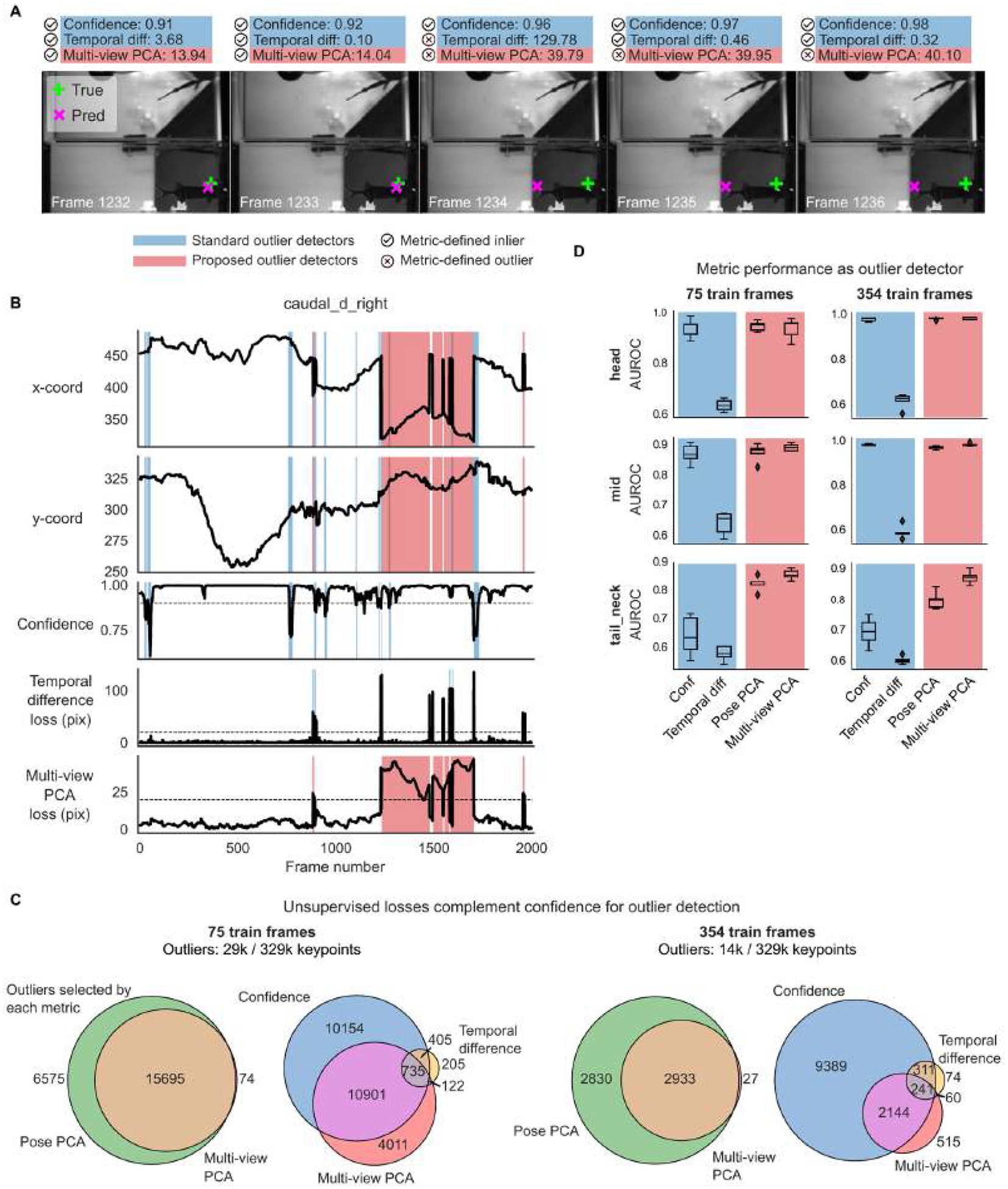
Example traces, unsupervised metrics, and predictions from a DeepLabCut model (trained on 354 frames) on held-out videos. Conventions for panels A-D as in Fig. 3. A: Example frame sequence. B: Example traces from the same video. C: Total number of keypoints flagged as outliers by each metric, and their overlap. D: Area under the receiver operating characteristic curve for several body parts. We define a ‘true outlier’ to be frames where the horizontal displacement between top and bottom predictions or the vertical displacement between top and right predictions exceeds 20 pixels. AUROC values are only shown for the three body parts that have corresponding keypoints across all three views included in the Pose PCA computation (many keypoints are excluded from the Pose PCA subspace due to many missing hand labels). AUROC values are computed across frames from 10 test videos; boxplot variability is over n=5 random subsets of training data. The same subset of keypoints is used for panel C. Boxes in panel D use 25th/50th/75th percentiles for min/center/max; whiskers extend to 1.5 * IQR.
Extended Data Fig. 2 |. Unsupervised losses complement model confidence for outlier detection on CRIM13 dataset.

Example traces, unsupervised metrics, and predictions from a DeepLabCut model (trained on 800 frames) on held-out videos. Conventions for panels A-C as in Fig. 3. A: Example frame sequence. B: Example traces from the same video. Because the size of CRIM13 frames are larger than those of the mirror-mouse and mirror-fish datasets, we use a threshold of 50 pixels instead of 20 to define outliers through the unsupervised losses. C: Total number of keypoints flagged as outliers by each metric, and their overlap. Outliers are collected from predictions across frames from 18 test videos and across predictions from five different networks trained on random subsets of labeled data.
Extended Data Fig. 3|. PCA-derived losses drive most improvements in semi-supervised models.

For each model type we train three networks with different random seeds controlling the data presentation order. The models train on 75 labeled frames and unlabeled videos. We plot the mean pixel error and 95% CI across keypoints and OOD frames, as a function of ensemble standard deviation, as in Fig. 4. At the 100% vertical line, n=17150 keypoints for mirror-mouse, n=18180 for mirror-fish, and n=89180 for CRIM13.
Extended Data Fig. 4 |. Unlabeled frames improve pose estimation in mirror-fish dataset.
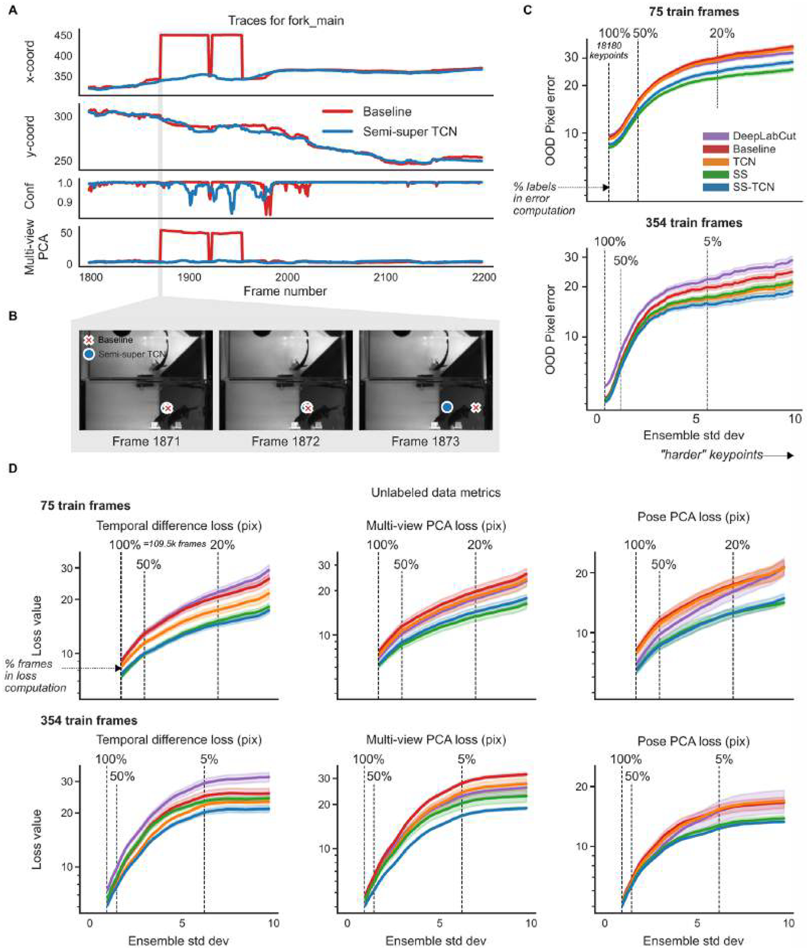
Conventions as in Fig. 4. A. Example traces from the baseline model and the semi-supervised TCN model (trained with 75 labeled frames) for a single keypoint on a held-out video (Supplementary Video 6). B. A sequence of frames corresponding to the grey shaded region in panel (A). C. Pixel error as a function of ensemble standard devation for scarce (top) and abundant (bottom) labeling regimes. D. Individual unsupervised loss terms plotted as a function of ensemble standard deviation for the scarce (top) and abundant (bottom) label regimes.
Extended Data Fig. 5 |. Unlabeled frames improve pose estimation in CRIM13 dataset.
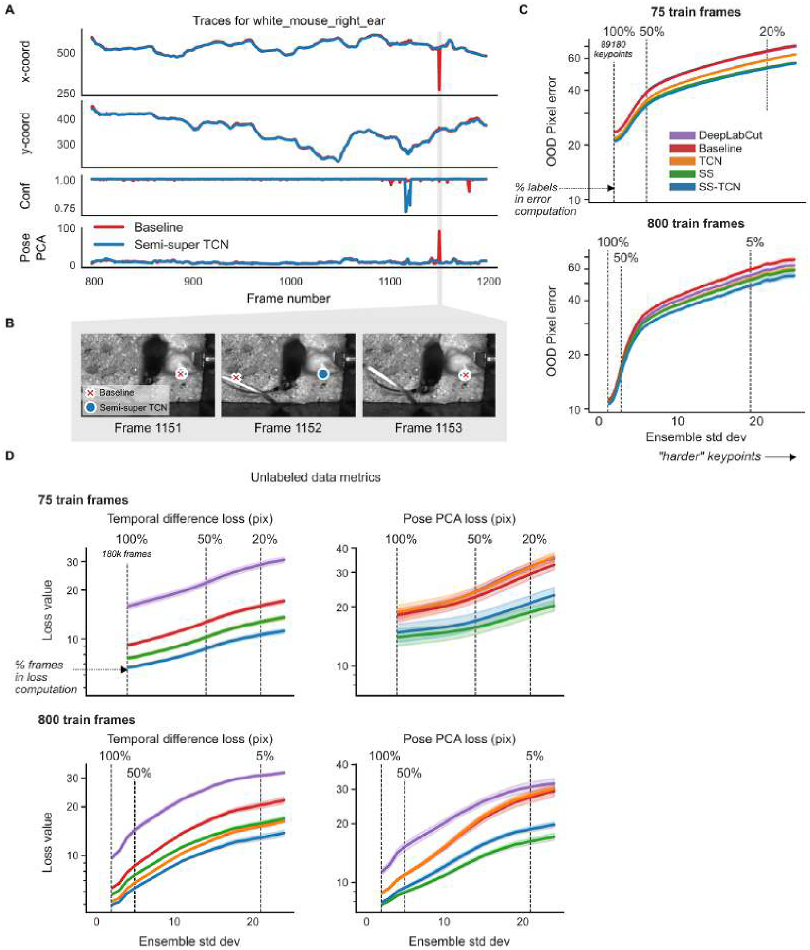
Conventions as in Fig. 4.A. Example traces from the baseline model and the semi-supervised TCN model (trained with 800 labeled frames) for a single keypoint on a held-out video (Supplementary Video 7). B. A sequence of frames corresponding to the grey shaded region in panel (A). C. Pixel error as a function of ensemble standard deviation for scarce (top) and abundant (bottom) labeling regimes. D. Individual unsupervised loss terms plotted as a function of ensemble standard deviation for the scarce (top) and abundant (bottom) labeling regimes.
Extended Data Fig. 6 ∣. The Ensemble Kalman Smoother improves pose estimation across datasets.
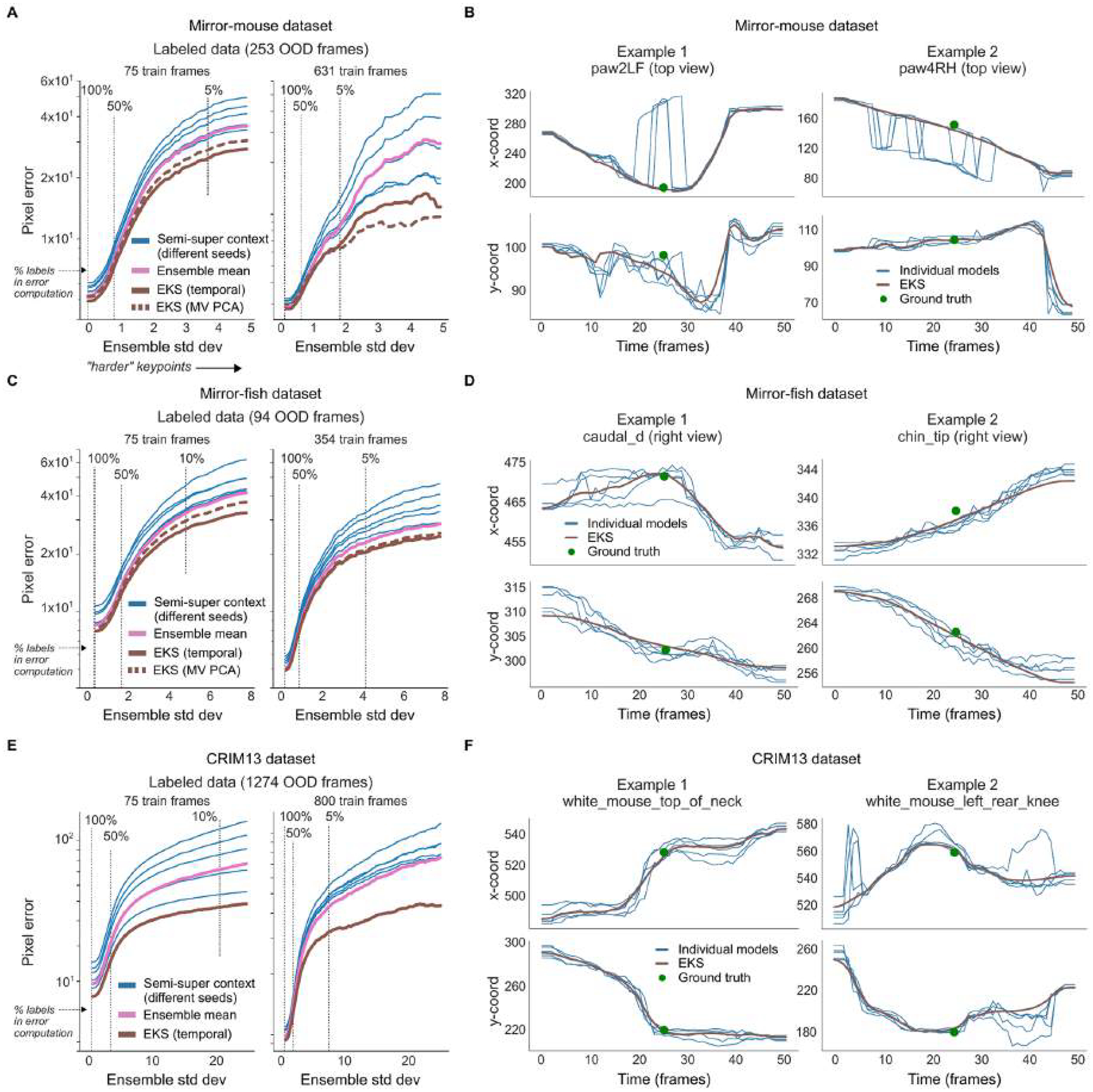
We trained an ensemble of five semi-supervised TCN models on the same training data. The networks differed in the order of data presentation and in the random weight initializations for their ‘head’. This figure complements Fig. 5 which uses an ensemble of DeepLabCut models as input to EKS. A. Mean OOD pixel error over frames and keypoints as a function of ensemble standard deviation (as in Fig. 4). B. Time series of predictions (x and y coordinates on top and bottom, respectively) from the five individual semi-supervised TCN models (75 labeled training frames; blue lines) and EKS-temporal (brown lines). Ground truth labels are shown as green dots. C,D. Identical to A,B but for the mirror-fish dataset. E,F. Identical to A,B but for the CRIM13 dataset.
Extended Data Fig. 7 |. Lightning Pose models and ensemble smoothing improve pose estimation on IBL paw data.

A. Sample frames from each camera view overlaid with a subset of paw markers estimated from DeepLabCut (left), Lightning Pose using a semi-supervised TCN model (center), and a 5-member ensemble using semi-supervised TCN models (right). B. Example left view frames from a subset of 44 IBL sessions. C. The empirical distribution of the right paw position from each view projected onto the 1D subspace of maximal correlation in a canonical correlation analysis (CCA). Column arrangement as in A. D. Correlation in the CCA subspace is computed across n=44 sessions for each model and paw. The LP+EKS model has a correlation of 1.0 by construction. E. Median right paw speed plotted across correct trials aligned to first movement onset of the wheel; error bars show 95% confidence interval across n=273 trials. The same trial consistency metric from Fig. 6 is computed. F. Trial consistency computed across n=44 sessions. G. Example traces of Kalman smoothed right paw speed (blue) and predictions from neural activity (orange) for several trials using cross-validated, regularized linear regression. H. Neural decoding performance across n=44 sessions. Panels D, F, and H use a one-sided Wilcoxon signed-rank test; boxes use 25th/50th/75th percentiles for min/center/max; whiskers extend to 1.5 * IQR. See Supplementary Table 2 for further quantification of boxes.
Extended Data Fig. 8 |. Lightning Pose enables easy model development, fast training, and is accessible via a cloud application.

A. Our software package outsources many tasks to existing tools within the deep learning ecosystem, resulting in a lighter, modular package that is easy to maintain and extend. The innermost purple box indicates the core components: accelerated video reading (via NVIDIA DALI), modular network design, and our general-purpose loss factory. The middle purple box denotes the training and logging operations which we outsource to PyTorch Lightning, and the outermost purple box denotes our use of the Hydra job manager. The right box depicts a rich set of interactive diagnostic metrics which are served via Streamlit and FiftyOne GUIs. B. A diagram of our cloud application. The application’s critical components are dataset curation, parallel model training, interactive performance diagnostics, and parallel prediction of new videos. C. Screenshots from our cloud application. From left to right: LabelStudio GUI for frame labeling, TensorFlow monitoring of training performance overlaying two different networks, FiftyOne GUI for comparing these two networks’ predictions on a video, and a Streamlit application that shows these two networks’ time series of predictions, confidences, and spatiotemporal constraint violations.
Supplementary Material
Acknowledgements
We thank P. Dayan and N. Steinmetz for serving on our IBL-paper board, as well as two anonymous reviewers whose detailed comments considerably strengthened our paper. We are grateful to N. Biderman for productive discussions and help with visualization. We thank M. Carandini and J. Portes for helpful comments; T. Abe, K. Buchanan and G. Pleiss for helpful discussions on ensembling; and H. Xiang for conversations on active learning and outlier detection. We thank W. Falcon, L. Antiga, T. Chaton and A. Wälchi (Lightning AI) for their technical support and advice on implementing our package and the cloud application. This work was supported by the following grants: Gatsby Charitable Foundation GAT3708 (to D.B., M.R.W., C.H., N.R.G., A.V., J.P.C. and L.P.), German National Academy of Sciences Leopoldina (to A.E.U.), Irma T Hirschl Trust (to N.B.S.), Netherlands Organisation for Scientific Research (VI.Veni.212.184; to A.E.U.), NSF IOS-2115007 (to N.B.S.), National Institutes of Health (NIH) K99NS128075 (to J.P.N.), NIH NS075023 (to N.B.S.), NIH NS118448 (to N.B.S.), NIH DK131086-02 (to N.B.S.), NIH U19NS123716 (to M.R.W.) and NSF 1707398 (to D.B., M.R.W., C.H., N.R.G., A.V., J.P.C. and L.P.), funds provided by the National Science Foundation and by DoD OUSD (R&E) under Cooperative Agreement PHY-2229929, The NSF AI Institute for Artificial and Natural Intelligence (to D.B., M.R.W., C.H., A.V., J.P.C. and L.P.), Simons Foundation (to M.R.W., M.M.S., J.M.H., A.K., G.T.M., J.P.N., A.P.V. and K.Z.S.) and the Wellcome Trust 216324 (M.M.S., J.M.H., A.K., G.T.M., J.P.N., A.P.V. and K.Z.S.). The funders had no role in study design, data collection and analysis, decision to publish or preparation of the manuscript.
The International Brain Laboratory
Larry Abbot10, Luigi Acerbi11, Valeria Aguillon-Rodriguez12, Mandana Ahmadi13, Jaweria Amjad13, Dora Angelaki14, Jaime Arlandis3, Zoe C. Ashwood15, Kush Banga16, Hailey Barrell17, Hannah M. Bayer10, Brandon Benson18, Julius Benson14, Jai Bhagat16, Dan Birman17, Niccolò Bonacchi3, Kcenia Bougrova3, Julien Boussard10, Sebastian A. Bruijns4, E. Kelly Buchanan10, Robert Campbell19, Matteo Carandini20, Joana A. Catarino3, Fanny Cazettes3, Gaelle A. Chapuis11, Anne K. Churchland21, Yang Dan22, Felicia Davatolhagh21, Peter Dayan4, Sophie Denève23, Eric E. J. DeWitt3, Ling Liang Dong24, Tatiana Engel15, Michele Fabbri10, Mayo Faulkner16, Robert Fetcho15, Ila Fiete24, Charles Findling11, Laura Freitas-Silva15, Surya Ganguli18, Berk Gercek11, Naureen Ghani19, Ivan Gordeliy23, Laura M. Haetzel24, Kenneth D. Harris16, Michael Hausser25, Naoki Hiratani13, Sonja Hofer19, Fei Hu22, Felix Huber11, Julia M. Huntenburg4, Cole Hurwitz10, Anup Khanal21, Christopher S. Krasniak12, Sanjukta Krishnagopal13, Michael Krumin16, Debottam Kundu4, Agnès Landemard20, Christopher Langdon15, Christopher Langfield10, Inês Laranjeira3, Peter Latham13, Petrina Lau25, Hyun Dong Lee10, Ari Liu24, Zachary F. Mainen3, Amalia Makri-Cottington25, Hernando Martinez-Vergara19, Brenna McMannon15, Isaiah McRoberts14, Guido T. Meijer3, Maxwell Melin21, Leenoy Meshulam26, Kim Miller17, Nathaniel J. Miska19, Catalin Mitelut10, Zeinab Mohammadi15, Thomas Mrsic-Flogel19, Masayoshi Murakami27, Jean-Paul Noel14, Kai Nylund17, Farideh Oloomi4, Alejandro Pan-Vazquez15, Liam Paninski10, Alberto Pezzotta13, Samuel Picard16, Jonathan W. Pillow15, Alexandre Pouget11, Florian Rau3, Cyrille Rossant16, Noam Roth17, Nicholas A. Roy15, Kamron Saniee10, Rylan Schaeffer24, Michael M. Schartner3, Yanliang Shi15, Carolina Soares19, Karolina Z. Socha20, Cristian Soitu12, Nicholas A. Steinmetz17, Karel Svoboda28, Marsa Taheri21, Charline Tessereau4, Anne E. Urai12, Erdem Varol10, Miles J. Wells16, Steven J. West19, Matthew R. Whiteway10, Charles Windolf10, Olivier Winter3, Ilana Witten15, Lauren E. Wool16, Zekai Xu13, Han Yu10, Anthony M. Zador12 & Yizi Zhang10
10Zuckerman Institute, Columbia University, New York, NY, USA. 11Department of Basic Neuroscience, University of Geneva, Geneva, Switzerland. 12Cold Spring Harbor Laboratory, Cold Spring Harbor, NY, USA. 13Gatsby Computational Neuroscience Unit, University College London, London, UK. 14Center for Neural Science, New York University, New York, NY, USA. 15Princeton Neuroscience Institute, Princeton University, Princeton, NJ, USA. 16Institute of Neurology, University College London, London, UK. 17Department of Biological Structure, University of Washington, Seattle, WA, USA. 18Department of Applied Physics, Stanford University, Stanford, CA, USA. 19Sainsbury-Wellcome Centre, University College London, London, UK. 20Institute of Opthalmology, University College London, London, UK. 21Department of Neurobiology, University of California, Los Angeles, Los Angeles, CA, USA. 22Department of Molecular and Cell Biology, University of California, Los Angeles, Berkeley, CA, USA. 23Département D’études Cognitives, école Normale Supérieure, Paris, France. 24Department of Brain and Cognitive Sciences, Massachusetts Institute of Technology, Cambridge, MA, USA. 25Wolfson Institute of Biomedical Research, University College London, London, UK. 26Center for Computational Neuroscience, University of Washington, Seattle, WA, USA. 27Department of Physiology, University of Yamanashi, Kofu, Yamanashi, Japan. 28The Allen Institute for Neural Dynamics, Seattle, Washington, WA, USA.
Footnotes
Code availability
The code for Lightning Pose is available at https://github.com/danbider/lightning-pose/ under the MIT license. The repository also contains a Google Colab tutorial notebook that trains a model, forms predictions on videos and visualizes the results. From the command-line interface, running pip install lightning-pose will install the latest release of Lightning Pose via the Python Package Index (PyPI).
The code for the EKS is available at https://github.com/paninski-lab/eks/ under the MIT license. The repository contains the core EKS code as well as scripts demonstrating how to use the code on several example datasets.
The code for the cloud-hosted application is available at https://github.com/Lightning-Universe/Pose-app/ under the Apache-2.0 license. This code enables launching our app locally or on cloud resources by creating a Lightning.ai account.
Code for reproducing the figures in the main text is available at https://github.com/themattinthehatt/lightning-pose-2024-nat-methods/ under the MIT license. This repository also includes a script for downloading all required data from the proper repositories.
The hardware and software used for IBL video collection is described elsewhere41. The protocols used in the mirror-mouse and mirror-fish datasets (both have the same video acquisition pipeline) are also described elsewhere14.
We used the following packages in our data analysis: CUDA toolkit (12.1.0), cuDNN (8.5.0.96), deeplabcut (2.3.5 for runtime benchmarking, 2.2.3 for everything else), ffmpeg (3.4.11), fiftyone (0.23.4), h5py (3.9.0), hydra-core (1.3.2), ibllib (2.32.3), imgaug (0.4.0), kaleido (0.2.1), kornia (0.6.12), lightning (2.1.0), lightning-pose (1.0.0), matplotlib (3.7.5), moviepy (1.0.3), numpy (1.24.4), nvidia-dali-cuda120 (1.28.0), opencv-python (4.9.0.80), pandas (2.0.3), pillow (9.5.0), plotly (5.15.0), scikit-learn (1.3.0), scipy (1.10.1), seaborn (0.12.2), streamlit (1.31.1), tensorboard (2.13.0) and torchvision (0.15.2).
Competing interests
R.S.L. assisted in the initial development of the cloud application as a solution architect at Lightning AI in Spring/Summer 2022. R.S.L. left the company in August 2022 and continues to hold shares. The remaining authors declare no competing interests.
Extended data is available for this paper at https://doi.org/10.1038/s41592-024-02319-1.
Supplementary information The online version contains supplementary material available at https://doi.org/10.1038/s41592-024-02319-1.
Data availability
All labeled data used in this paper are publicly available.
mirror-mouse https://doi.org/10.6084/m9.figshare.24993315.v1 (ref. 71)
mirror-fish https://doi.org/10.6084/m9.figshare.24993363.v1 (ref.72)
CRIM13 https://doi.org/10.6084/m9.figshare.24993384.v1 (ref. 73)
All of the model predictions on labeled frames and unlabeled videos are available via Figshare at https://doi.org/10.6084/m9.figshare.25412248.v2 (ref. 74). These results, along with the labeled data, can be used to reproduce the main figures of the paper.
To access the IBL data analyzed in Fig. 6 and Extended Data Fig. 7, see the documentation at https://int-brain-lab.github.io/ONE/FAQ.html#how-do-i-download-the-datasets-cache-for-a-specific-ibl-paper-release and use the tag 2023_Q1_Biderman_Whiteway_et_al. This will provide access to spike-sorted neural activity, trial timing variables (stimulus onset, feedback delivery and so on), the original IBL DeepLabCut traces and the raw videos.
References
- 1.Krakauer JW, Ghazanfar AA, Gomez-Marin A, Maclver MA & Poeppel D Neuroscience needs behavior: correcting a reductionist bias. Neuron 93, 480–490 (2017). [DOI] [PubMed] [Google Scholar]
- 2.Branson K, Robie AA, Bender J, Perona P & Dickinson MH High-throughput ethomics in large groups of Drosophila. Nat. Methods 6, 451–457 (2009). [DOI] [PMC free article] [PubMed] [Google Scholar]
- 3.Berman GJ, Choi DM, Bialek W & Shaevitz JW Mapping the stereotyped behaviour of freely moving fruit flies. J. Royal Soc. Interface 11, 20140672 (2014). [DOI] [PMC free article] [PubMed] [Google Scholar]
- 4.Wiltschko AB et al. Mapping sub-second structure in mouse behavior. Neuron 88, 1121–1135 (2015). [DOI] [PMC free article] [PubMed] [Google Scholar]
- 5.Wiltschko AB et al. Revealing the structure of pharmacobehavioral space through motion sequencing. Nat. Neurosci 23, 1433–1443 (2020). [DOI] [PMC free article] [PubMed] [Google Scholar]
- 6.Luxem K et al. Identifying behavioral structure from deep variational embeddings of animal motion. Commun. Biol 5, 1267 (2022). [DOI] [PMC free article] [PubMed] [Google Scholar]
- 7.Mathis A et al. Deeplabcut: markerless pose estimation of user-defined body parts with deep learning. Nat. Neurosci 21, 1281–1289 (2018). [DOI] [PubMed] [Google Scholar]
- 8.Pereira TD et al. Fast animal pose estimation using deep neural networks. Nat. Methods 16, 117–125 (2019). [DOI] [PMC free article] [PubMed] [Google Scholar]
- 9.Graving JM et al. Deepposekit, a software toolkit for fast and robust animal pose estimation using deep learning. Elife 8, e47994 (2019). [DOI] [PMC free article] [PubMed] [Google Scholar]
- 10.Dunn TW et al. Geometric deep learning enables 3D kinematic profiling across species and environments. Nat. Methods 18, 564–573 (2021). [DOI] [PMC free article] [PubMed] [Google Scholar]
- 11.Chen Z et al. Alphatracker: a multi-animal tracking and behavioral analysis tool. Front. Behav. Neurosci 17, 1111908 (2023). [DOI] [PMC free article] [PubMed] [Google Scholar]
- 12.Jones JM et al. A machine-vision approach for automated pain measurement at millisecond timescales. Elife 9, e57258 (2020). [DOI] [PMC free article] [PubMed] [Google Scholar]
- 13.Padilla-Coreano N et al. Cortical ensembles orchestrate social competition through hypothalamic outputs. Nature 603, 667–671 (2022). [DOI] [PMC free article] [PubMed] [Google Scholar]
- 14.Warren RA et al. A rapid whisker-based decision underlying skilled locomotion in mice. Elife 10, e63596 (2021). [DOI] [PMC free article] [PubMed] [Google Scholar]
- 15.Hsu AI & Yttri EA B-SOiD, an open-source unsupervised algorithm for identification and fast prediction of behaviors. Nat. Commun 12, 5188 (2021). [DOI] [PMC free article] [PubMed] [Google Scholar]
- 16.Pereira TD et al. Sleap: a deep learning system for multi-animal pose tracking. Nat. Methods 19, 486–495 (2022). [DOI] [PMC free article] [PubMed] [Google Scholar]
- 17.Weinreb C et al. Keypoint-MoSeq: parsing behavior by linking point tracking to pose dynamics. Preprint at bioRxiv 10.1101/2023.03.16.532307 (2023). [DOI] [PMC free article] [PubMed] [Google Scholar]
- 18.Karashchuk P et al. Anipose: a toolkit for robust markerless 3D pose estimation. Cell Rep 36, 109730 (2021). [DOI] [PMC free article] [PubMed] [Google Scholar]
- 19.Monsees A et al. Estimation of skeletal kinematics in freely moving rodents. Nat. Methods 19, 1500–1509 (2022). [DOI] [PMC free article] [PubMed] [Google Scholar]
- 20.Rodgers CC A detailed behavioral, videographic, and neural dataset on object recognition in mice. Sci. Data 9, 620 (2022). [DOI] [PMC free article] [PubMed] [Google Scholar]
- 21.Chapelle O, Schölkopf B & Zien A (eds) Semi-Supervised Learning (The MIT Press, 2006). [Google Scholar]
- 22.Lakshminarayanan B, Pritzel A & Blundell C Simple and scalable predictive uncertainty estimation using deep ensembles. in Advances in Neural Information Processing Systems vol. 30 (eds Guyon I et al.) (Curran Associates, 2017). [Google Scholar]
- 23.Abe T et al. Neuroscience cloud analysis as a service: An open-source platform for scalable, reproducible data analysis. Neuron 110, 2771–2789 (2022). [DOI] [PMC free article] [PubMed] [Google Scholar]
- 24.Falcon W et al. Pytorchlightning/pytorch-lightning: 0.7.6 release Zenodo; 10.5281/zenodo.3828935 (2020). [DOI] [Google Scholar]
- 25.Recht B, Roelofs R, Schmidt L & Shankar V Do imagenet classifiers generalize to imagenet? In International Conference on Machine Learning, 5389–5400 (PMLR, 2019). [Google Scholar]
- 26.Tran D et al. Plex: Towards reliability using pretrained large model extensions. Preprint at https://arxiv.org/abs/2207.07411 (2022).
- 27.Burgos-Artizzu XP, Dollár P, Lin D, Anderson DJ & Perona P Social behavior recognition in continuous video. In 2012 IEEE Conference on Computer Vision and Pattern Recognition, 1322–1329 (IEEE, 2012). [Google Scholar]
- 28.Segalin C et al. The mouse action recognition system (mars) software pipeline for automated analysis of social behaviors in mice. Elife 10, e63720 (2021). [DOI] [PMC free article] [PubMed] [Google Scholar]
- 29.IBL. Data release - Brainwide map - Q4 2022 (2023). Figshare; 10.6084/m9.figshare.21400815.v6 (2022). [DOI] [Google Scholar]
- 30.Desai N et al. Openapepose, a database of annotated ape photographs for pose estimation. Elife 12, RP86873 (2023). [DOI] [PMC free article] [PubMed] [Google Scholar]
- 31.Syeda A et al. Facemap: a framework for modeling neural activity based on orofacial tracking. Nat. Neurosci 27, 187–195 (2024). [DOI] [PMC free article] [PubMed] [Google Scholar]
- 32.Spelke ES Principles of object perception. Cogn. Sci 14, 29–56 (1990). [Google Scholar]
- 33.Wu A et al. Deep graph pose: a semi-supervised deep graphical model for improved animal pose tracking. in Advances in Neural Information Processing Systems (eds Larochelle H et al.) 6040–6052 (2020). [Google Scholar]
- 34.Nath T et al. Using deeplabcut for 3D markerless pose estimation across species and behaviors. Nat. Protoc 14, 2152–2176 (2019). [DOI] [PubMed] [Google Scholar]
- 35.Zhang Y & Park HS Multiview supervision by registration. In Proceedings of the IEEE/CVF Winter Conference on Applications of Computer Vision, 420–428 (2020). [Google Scholar]
- 36.He Y, Yan R, Fragkiadaki K & Yu S-I Epipolar transformers. In Proceedings of the IEEE/CVF Conference on Computer Vision and Pattern Recognition, 7779–7788 (2020). [Google Scholar]
- 37.Hartley R & Zisserman A Multiple View Geometry in Computer Vision (Cambridge University Press, 2003). [Google Scholar]
- 38.Bialek W On the dimensionality of behavior. Proc. Natl Acad. Sci. uSA 119, e2021860119 (2022). [DOI] [PMC free article] [PubMed] [Google Scholar]
- 39.Stephens GJ, Johnson-Kerner B, Bialek W & Ryu WS From modes to movement in the behavior of caenorhabditis elegans. PloS ONE 5, e13914 (2010). [DOI] [PMC free article] [PubMed] [Google Scholar]
- 40.Yan Y, Goodman JM, Moore DD, Solla SA & Bensmaia SJ Unexpected complexity of everyday manual behaviors. Nat. Commun 11, 3564 (2020). [DOI] [PMC free article] [PubMed] [Google Scholar]
- 41.IBL. Video hardware and software for the international brain laboratory. Figshare 10.6084/m9.figshare.19694452.v1 (2022). [DOI] [Google Scholar]
- 42.Li T, Severson KS, Wang F & Dunn TW Improved 3Dd markerless mouse pose estimation using temporal semi-supervision. Int. J. Comput. Vis 131, 1389–1405 (2023). [DOI] [PMC free article] [PubMed] [Google Scholar]
- 43.Beluch WH, Genewein T, Nürnberger A & Köhler JM The power of ensembles for active learning in image classification. In Proceedings of the IEEE Conference on Computer Vision and Pattern Recognition, 9368–9377 (2018). [Google Scholar]
- 44.Abe T, Buchanan EK, Pleiss G, Zemel R & Cunningham JP Deep ensembles work, but are they necessary? in Advances in Neural Information Processing Systems 35, 33646–33660 (2022). [Google Scholar]
- 45.Bishop CM & Nasrabadi NM Pattern Recognition and Machine Learning, vol. 4 (Springer, 2006). [Google Scholar]
- 46.Yu H et al. AP-10K: a benchmark for animal pose estimation in the wild. Preprint at https://arxiv.org/abs/2108.12617 (2021).
- 47.Ye S et al. SuperAnimal models pretrained for plug-and-play analysis of animal behavior. Preprint at https://arxiv.org/abs/2203.07436 (2022).
- 48.Zheng C et al. Deep learning-based human pose estimation: a survey. ACM Computing Surveys 56, 1–37 (2023). [Google Scholar]
- 49.Lin T-Y et al. Microsoft coco: common objects in context. In Computer Vision–ECCV 2014: 13th European Conference, Zurich, Switzerland, September 6–12, 2014, Proceedings. Vol. 8693, 740–755 (Springer, 2014). [Google Scholar]
- 50.Ionescu C, Papava D, Olaru V & Sminchisescu C Human3. 6M: large scale datasets and predictive methods for 3D human sensing in natural environments. IEEE Trans. Pattern Anal. Mach. Intell 36, 1325–1339 (2013). [DOI] [PubMed] [Google Scholar]
- 51.Loper M, Mahmood N, Romero J, Pons-Moll G & Black MJ SMPL: a skinned multi-person linear model. In Seminal Graphics Papers: Pushing the Boundaries. Vol. 2, 851–866 (2023). [Google Scholar]
- 52.Marshall JD, Li T, Wu JH & Dunn TW Leaving flatland: advances in 3D behavioral measurement. Curr. Opin. Neurobiol 73, 102522 (2022). [DOI] [PubMed] [Google Scholar]
- 53.Günel S et al. DeepFly3D, a deep learning-based approach for 3D limb and appendage tracking in tethered, adult Drosophila. Elife 8, e48571 (2019). [DOI] [PMC free article] [PubMed] [Google Scholar]
- 54.Sun JJ et al. BKinD-3D: self-supervised 3D keypoint discovery from multi-view videos. In Proceedings of the IEEE/CVF Conference on Computer Vision and Pattern Recognition, 9001–9010 (2023). [DOI] [PMC free article] [PubMed] [Google Scholar]
- 55.Bala PC et al. Automated markerless pose estimation in freely moving macaques with openmonkeystudio. Nat. Commun 11, 4560 (2020). [DOI] [PMC free article] [PubMed] [Google Scholar]
- 56.Hinton G, Vinyals O & Dean J Distilling the knowledge in a neural network. Preprint at https://arxiv.org/abs/1503.02531 (2015).
- 57.Lauer J et al. Multi-animal pose estimation, identification and tracking with deeplabcut. Nat. Meth 19, 496–504 (2022). [DOI] [PMC free article] [PubMed] [Google Scholar]
- 58.Chettih SN, Mackevicius EL, Hale S & Aronov D Barcoding of episodic memories in the hippocampus of a food-caching bird. Cell 187, 1922–1935 (2024). [DOI] [PMC free article] [PubMed] [Google Scholar]
- 59.IBL et al. Standardized and reproducible measurement of decision-making in mice. Elife 10, e63711 (2021). [DOI] [PMC free article] [PubMed] [Google Scholar]
- 60.IBL et al. Reproducibility of in vivo electrophysiological measurements in mice. Preprint at bioRxiv 10.1101/2022.05.09.491042 (2022). [DOI] [Google Scholar]
- 61.Paszke A et al. Pytorch: An imperative style, high-performance deep learning library. in Advances in Neural Information Processing Systems 32, 8024–8035 (2019). [Google Scholar]
- 62.Jafarian Y, Yao Y & Park HS MONET: multiview semi-supervised keypoint via epipolar divergence. Preprint at https://arxiv.org/abs/1806.00104 (2018).
- 63.Tresch MC & Jarc A The case for and against muscle synergies. Curr. Opin. Neurobiol 19, 601–607 (2009). [DOI] [PMC free article] [PubMed] [Google Scholar]
- 64.Stephens GJ, Johnson-Kerner B, Bialek W & Ryu WS Dimensionality and dynamics in the behavior of C. elegans. PLoS Comput. Biol 4, e1000028 (2008). [DOI] [PMC free article] [PubMed] [Google Scholar]
- 65.Kingma DP & Ba J Adam: A method for stochastic optimization. Preprint at https://arxiv.org/abs/1412.6980 (2014). [Google Scholar]
- 66.Virtanen P et al. Scipy 1.0: fundamental algorithms for scientific computing in Python. Nat. Methods 17, 261–272 (2020). [DOI] [PMC free article] [PubMed] [Google Scholar]
- 67.IBL et al. A brain-wide map of neural activity during complex behaviour. Preprint at bioRxiv 10.1101/2023.07.04.547681 (2023). [DOI] [PMC free article] [PubMed] [Google Scholar]
- 68.Pedregosa F et al. Scikit-learn: machine learning in Python. J. Mach. Learn. Res 12, 2825–2830 (2011). [Google Scholar]
- 69.Zolnouri M, Li X & Nia VP Importance of data loading pipeline in training deep neural networks. Preprint at https://arxiv.org/abs/2005.02130 (2020).
- 70.Yadan O Hydra - a framework for elegantly configuring complex applications. Github; https://github.com/facebookresearch/hydra (2019). [Google Scholar]
- 71.Whiteway M, Biderman D, Warren R, Zhang Q & Sawtell NB Lightning Pose dataset: mirror-mouse. Figshare; 10.6084/m9.figshare.24993315.v1 (2024). [DOI] [Google Scholar]
- 72.Whiteway M et al. Lightning Pose dataset: mirror-fish. Figshare; 10.6084/m9.figshare.24993363.v1 (2024). [DOI] [Google Scholar]
- 73.Whiteway M & Biderman D Lightning Pose dataset: CRIM13. Figshare; 10.6084/m9.figshare.24993384.v1 (2024). [DOI] [Google Scholar]
- 74.Whiteway M & Biderman D Lightning Pose results: Nature Methods 2024. Figshare; 10.6084/m9.figshare.25412248.v2 (2024). [DOI] [Google Scholar]
Associated Data
This section collects any data citations, data availability statements, or supplementary materials included in this article.
Supplementary Materials
Data Availability Statement
All labeled data used in this paper are publicly available.
mirror-mouse https://doi.org/10.6084/m9.figshare.24993315.v1 (ref. 71)
mirror-fish https://doi.org/10.6084/m9.figshare.24993363.v1 (ref.72)
CRIM13 https://doi.org/10.6084/m9.figshare.24993384.v1 (ref. 73)
All of the model predictions on labeled frames and unlabeled videos are available via Figshare at https://doi.org/10.6084/m9.figshare.25412248.v2 (ref. 74). These results, along with the labeled data, can be used to reproduce the main figures of the paper.
To access the IBL data analyzed in Fig. 6 and Extended Data Fig. 7, see the documentation at https://int-brain-lab.github.io/ONE/FAQ.html#how-do-i-download-the-datasets-cache-for-a-specific-ibl-paper-release and use the tag 2023_Q1_Biderman_Whiteway_et_al. This will provide access to spike-sorted neural activity, trial timing variables (stimulus onset, feedback delivery and so on), the original IBL DeepLabCut traces and the raw videos.