Development of a novel extension of Rayleigh distribution with application to COVID-19 data

Abstract

Effective analysis of medical data is essential for understanding complex healthcare phenomena. Probability distribution models offer a structured approach to uncover patterns in such data, particularly for studying disease progression, survival analysis and many more. In this study, we explore a novel probability distribution model, derived by applying the DUS transformation to the standard Rayleigh distribution. We thoroughly investigate the statistical properties of the proposed model and derive key reliability measures to demonstrate its applicability in reliability analysis. To ensure precise parameter estimation, various estimation methods are evaluated, and their effectiveness is assessed through a detailed simulation study using bias, mean squared error, and mean relative error as performance criteria. The developed model’s practical applicability is demonstrated with an analysis of COVID-19 data, comparing its performance with several well-known distributions. The results highlight the flexibility and accuracy of the model, establishing it as a powerful and reliable tool for advanced statistical modelling in healthcare research.

Introduction

In the realm of medical science, the accurate analysis and interpretation of data are crucial for advancing healthcare outcomes, improving treatment strategies, and enhancing clinical decision-making. Medical data, however, is often complex, high-dimensional, and riddled with uncertainties arising from biological variability, environmental influences, and limitations in data collection. To address these challenges, probability distribution models provide a powerful and flexible approach for analysing and interpreting medical data. These models not only account for the inherent randomness in medical phenomena but also offer structured ways to quantify uncertainty, predict outcomes, and make evidence-based decisions. This research article focuses on the application of probability distribution models in the context of medical science data with special reference to COVID-19. The COVID-19 pandemic has underscored the importance of effective data analysis in medical science, particularly in understanding the spread, impact, and mitigation of infectious diseases. Such data encompassing infection rates, recovery times, mortality, and transmission patterns, is inherently stochastic, meaning it involves elements of randomness. Probability distributions provide a framework for modelling these random phenomena and understanding their behaviour over time. By fitting appropriate distributions to the observed data, researchers can predict outcomes like future case counts, hospitalization rates, or the probability of transmission under different conditions. Thus, from modelling disease spread and patient survival rates to assessing treatment efficiency and risk factors, probability distribution models play a vital role in capturing real-world variability in clinical and epidemiological data.

In recent years, researchers have increasingly focused on developing families of probability distributions for modelling medical data. Notable contributions in this area include the innovative lifetime distribution introduced by Almongy et al.¹, which merges the Rayleigh distribution with the extended odd Weibull family to form the extended odd Weibull Rayleigh distribution, specifically aimed at modelling COVID-19 mortality rates. Additionally, Sindhu et al.² explored a generalization of the Gumbel type-II distribution for analysing COVID-19 data, while in another study Sindhu et al.³ developed an exponentiated transformation of Gumbel type-II to handle two datasets of COVID-19 death cases. Liu et al.⁴ proposed a novel statistical model known as the arcsine modified Weibull distribution, demonstrating its effectiveness through COVID-19 data modelling. Kilai et al.⁵ introduced a new flexible statistical model for analysing COVID-19 mortality rates. Hossam et al.⁶ presented an extension of the Gumbel distribution, incorporating a new alpha power transformation method to enhance its application to COVID-19 data. Gemeay et al.⁷ contributed by proposing a two-parameter statistical distribution, combining exponential and gamma distributions, and demonstrated its superiority using COVID-19 datasets. Recently, Alomair et al.⁸ introduced the exponentiated XLindley distribution, showcasing its applicability through three real-world datasets, including COVID-19 mortality rates, precipitation measurements, and failure times for repairable items. Further advancements in probability distributions include the exponentiated Chen distribution, as examined by Dey et al.⁹, who investigated its properties and estimation methods while applying it to real-world datasets to assess its potential for statistical analysis. Additionally, Dey et al.¹⁰ studied the generalized exponential distribution, particularly in relation to ozone data. Rather and Subramanian¹¹ introduced the exponentiated Mukherjee-Islam distribution, demonstrating its efficiency through real-world applications. Following this, Rather and Özel¹² explored the weighted Power Lindley distribution. Moreover, Rather and Özel¹³ continued their work with the study of a new length-biased Power Lindley distribution, including an analysis of its properties and applications. Rather et al.¹⁴ proposed a new class of probability distribution called the exponentiated Ailamujia distribution, finding that it offers a superior fit compared to traditional distributions. Singh et al.¹⁵ examined the exponentiated Nadarajah–Haghighi distribution, while Ahmad et al.¹⁶ developed a novel Sin-G class of distributions, including an illustration involving the Lomax distribution. Qayoom and Rather¹⁷ contributed by exploring the Weighted Transmuted Mukherjee-Islam distribution, along with a comprehensive study of the length-biased Transmuted distribution¹⁸ as an extension of the Mukherjee-Islam distribution.

In this research article, we aim to develop a new extension of the Rayleigh distribution using the DUS transformation approach initially proposed by Kumar et al.¹⁹. The DUS transformation has been extensively studied by numerous researchers to create enhanced probability models for the analysis and interpretation of real-world data. Notable contributions in this area include those by Tripathi et al.²⁰, Abujarad et al.²¹, Kavya and Manoharan²², Gul et al.²³, Deepti and Chacko²⁴, Gauthami and Chacko²⁵, Karakaya et al.²⁶, Thomas and Chacko²⁷ and Gül et al.²⁸. More recently, Qayoom et al.²⁹ extended the DUS transformation to the Lindley distribution, demonstrating its utility in evaluating and enhancing system reliability.

New extension of Rayleigh distribution

The Rayleigh distribution is a continuous probability distribution named after the British Scientist Lord Rayleigh³⁰ and is characterized by its scale parameter, which influences the shape and spread of the data. The distribution is widely utilized across various fields, including life testing experiments, communication theory, medical testing and clinical studies, reliability analysis, applied statistics and many more fields. Given its importance and the aim to enhance its versatility, several researchers have proposed extensions to the Rayleigh distribution. Notably, Kundu and Raqab³¹ introduced the generalized Rayleigh distribution. MirMostafaee et al.³² presented a new extension called the Marshall–Olkin extended generalized Rayleigh distribution, which builds on the framework established by Marshall and Olkin³³. Additionally, Rashwan³⁴ examined the Kumaraswamy Rayleigh distribution. Further contributions include Ateeq et al.³⁵, who derived the Rayleigh-Rayleigh distribution (RRD) using the transformed transformer technique. Bantan et al.³⁶ explored the Unit-Rayleigh distribution, assessing its significance through real-life datasets. Falgore et al.³⁷ developed the inverse Lomax-Rayleigh distribution for modelling medical data. More recently, Ahmad et al.³⁸ introduced a new family of distributions inspired by the hyperbolic Sine function generator, with the Rayleigh distribution serving as the base for the newly established hyperbolic Sine-Rayleigh distribution.

Consider a random variable following Rayleigh distribution with parameter , then the probability density function (PDF) of is given by

Here is the scale parameter characterizing the shape and spread of the distribution. The associated cumulative distribution function (CDF) is given by .

In this section, we will generalize the PDF of Rayleigh distribution by following DUS transformation approach suggested by Kumar et al.¹⁹. So, the PDF of the new generalized Rayleigh distribution is

1

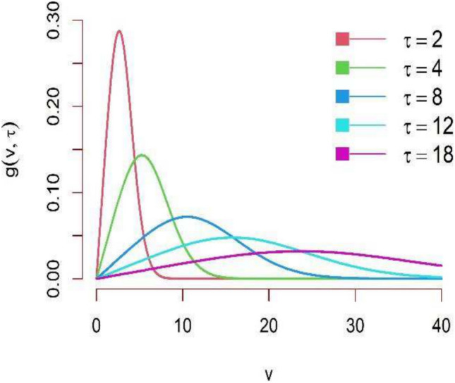
From now onwards this new generalized Rayleigh distribution expressed by Eq. (1) will be called as DUS Rayleigh distribution. Tripathi and Agiwal³⁹ have also studied and discussed this new generalization of Rayleigh distribution. The behavior of the DUS Rayleigh distribution for different values of its parameter is graphically presented in Figs. 1 and 2 as below:

Fig. 1.

PDF plot of DUS Rayleigh distribution for different parameter values.

Fig. 2.

PDF plot of DUS Rayleigh distribution for different parameter values.

From the above graphical representation of the PDF of DUS Rayleigh distribution, it can be observed that the distribution is positively skewed (right-skewed), that is, longer tail on the right. For small , the curve is sharply peaked near small values of variable V, indicating that most values are concentrated in a narrow range around the mode of the distribution. For large , the curve becomes more stretched out, with a broader range of values. This implies that the values are less concentrated around the mode.

The corresponding cumulative distribution function (CDF) of DUS Rayleigh distribution is given by

2

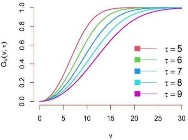
The graphical representation of the CDF of DUS Rayleigh distribution is shown in Figs. 3 and 4.

Fig. 3.

CDF plot of DUS Rayleigh distribution for different parameter values.

Fig. 4.

CDF plot of DUS Rayleigh distribution for different parameter values.

It can be observed that the CDF Curve stretches in between 0 and 1. This implies that the expression 4 is a valid CDF. From the graphical representation of the CDF of DUS Rayleigh distribution, the CDF shifts right as increases. This means that for the same value of given random variable V, the probability of finding a value below decreases. For small , the curve rises steeply at small values of , meaning that most values are clustered around a lower range. For large , the curve shifts right, meaning that values are more spread out and higher values are more likely, that is, the probability of small values is lower. In other words, it can be interpreted that larger values make the CDF increase more gradually, spreading the probability over a wider range.

Statistical properties

In this section, some of the general statistical properties of the newly developed probability distribution will be explored. These properties include quantile function, moments of the distribution, coefficient of variation, measure of skewness, measure of kurtosis and incomplete moments. In this section, we will also compute moment generating function, characteristics function and cumulant generating function for the explored DUS Rayleigh distribution.

Quantile function

A quantile function provides the value below which a given percentage of data falls. Given a cumulative distribution function such that of a continuous random variable , then the quantile function denoted by for is defined as

For the DUS Rayleigh distribution, the quantile function is obtained by determining the value of for which , that is

which is the required expression of quantile function for DUS Rayleigh distribution and is very essential for assessing behaviour of the distribution with the help of simulation study.

Moments

Moments are essential mathematical tools used to describe and analyze the properties of datasets or mathematical functions, offering a mathematical framework to capture essential properties like central tendency, spread (variability) and shape. Their versatility makes them indispensable across diverse fields, enabling deeper insights and more precise predictions in both theoretical and applied research.

Now, the moment about origin of the given model is

Using Eq. (1) in the above expression, we get

Put , so .

When and, when , therefore

3

Putting in Eq. (3) we obtain first four moments about origin and are expressed as

So, the variance and coefficient of variation for the given model respectively are calculated as

and

Moreover, the coefficient of skewness and the coefficient of kurtosis for the explored model are given by

The behavior of the mean, variance, C.V, coefficient of skewness and kurtosis for the DUS Rayleigh distribution for different values of the parameter involved in the distribution is presented in Table 1 below:

Table 1.

Mean, variance, C.V, coefficient of skewness and kurtosis for given model for different values of the parameter.

Parameter	Mean ()	Variance ()	C.V.
	0.01439237	0.00004625	0.4725073	0.4098242	2.878333
	0.07190761	0.00112819	0.4671059	0.4113968	2.947856
	0.1428335	0.00443713	0.4663598	0.4423789	3.021732
	0.2876621	0.01814687	0.4682935	0.4623289	3.103902
	0.4344241	0.04092956	0.4656983	0.4141835	3.012301
	0.5767866	0.07600831	0.4779862	0.453753	2.990883
	0.7209114	0.1131175	0.4665337	0.3991438	2.923794
	0.8589164	0.1646991	0.4724923	0.4249324	3.004540
	1.0046350	0.2253588	0.4725297	0.4459983	2.978124
	1.073314	0.2552967	0.4707561	0.444598	3.054514
	1.148572	0.2841372	0.4640938	0.4261991	3.043443
	1.290832	0.3598193	0.4646997	0.4171002	2.986071
	1.435767	0.4492511	0.4668319	0.4234487	2.985700
	1.801118	0.7035152	0.4656876	0.3932215	2.882782
	2.168426	1.0554980	0.4737880	0.4604522	3.097167
	2.517197	1.3993120	0.4699374	0.4523078	2.985927
	2.855038	1.8414670	0.4753025	0.4931543	3.182636

Incomplete moments

The incomplete moment about origin for the given model is given by

After following the steps used in the computation of moments of the distribution, the resultant expression for incomplete moments is given by

Moment generating function

The moment generating function of the given model is computed as

Similarly, the characteristics function and cumulant generating function of given model are given by

Reliability analysis measures

In this section we will explain various measures needed for studying reliability analysis to evaluate the performance of a component or system. These measures include survival function, hazard rate, mean residual life, mean past life, and stress-strength reliability. All these measures will be derived in relation to the DUS Rayleigh distribution.

Survival function and hazard function

The survival function for the DUS Rayleigh distribution is given by

It can be further simplified as

The graphical behaviour of the survival function for different parameter values is illustrated in Figs. 5 and 6. It can be observed from graphical representation of the survival function based on DUS Rayleigh distribution that for small , the survival function declines sharply, indicating that failures occur early and survival probability decreases rapidly. This can be interpreted as the system has low reliability and short lifespan. On the other hand for large , the survival function shifts right and declines more slowly, implies that failures are spread over a longer duration and survival remains high for a longer time. This indicates that the system is more reliable, with a longer lifespan.

Fig. 5.

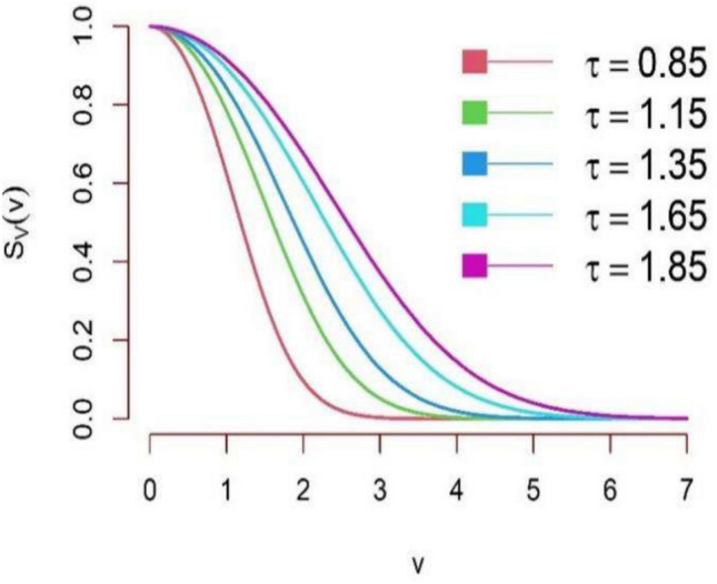
Survival function plot of DUS Rayleigh distribution.

Fig. 6.

Survival function plot of DUS Rayleigh distribution.

The hazard function based on DUS Rayleigh distributions expressed as a ratio of PDF of DUS Rayleigh distribution and its survival function. Mathematically, it is expressed as

Mean residual life

Mean residual life (MRL) is a measure that describe “the expected remaining lifetime of a system, component or individual given that it has survived up to a certain time point”. In simple words MRL states “How much more time can the system be expected to function, given that it is still operational at time ”. Mathematically, for a non-negative random variable denoting the failure time of a component or system and follows DUS Rayleigh distribution, then the MRL at time is given by

On substituting the expression of PDF of DUS Rayleigh distribution shown in Eq. (1), the MRL at time becomes

Let , then .

When and when , therefore

where, represents the CDF of DUS Rayleigh distribution given in Eq. (2).

Mean past life

The mean past life (MPL) at time measures “the expected amount of time that the system or component has already operated, given that it is still functioning at time ”. In other words, it explains “how long has the system or component been operating on average, given that it is still functioning at time ”. Suppose that the non-negative random variable denoting the failure time of a component or system follows DUS Rayleigh distribution. Then the MPL is given by

Using Eq. (1), then MPL can be expressed as

Let , then .

When and when , therefore

Where, denotes the CDF of DUS Rayleigh distribution given in Eq. (2).

Stress-strength reliability

Stress-strength reliability provides an estimate of the probability that a component or system will not fail when exposed to a given stress or load. The purpose is to compare strength with stress, that is, the capacity of the system to withstand the actual load applied to the component or system. This approach is essential in designing reliable products as it accounts for the variability in both stress and strength distribution.

Let the random variable represents the strength of the component or system, that is, the maximum load or pressure a component or system can endure and let the random variable denotes the stress level, that is, the actual load that the component experiences in operation. Then stress-strength reliability (say) is the probability that the strength exceeds the stress and is mathematically expressed as

Under the assumption that and follows DUS Rayleigh distribution with parameters and respectively. Therefore, the stress-strength reliability can be written as .

After simplification we get

Order statistics

Let be a random sample of size attaining the values from DUS Rayleigh distribution. Order statistics simply represents the ordered values of the data set. So, the ordered statistics for the given random sample is enumerated as

where,

, and .

The PDF of ordered statistics for DUS Rayleigh is given by

On using Eqs. (1) and (2), then the above expression of the PDF of ordered statistics becomes

4

On substituting in Eq. (4), we get the PDF of minimum and maximum ordered statistics respectively for the given model and are expressed as.

Entropy measures

Entropy is a fundamental concept in statistics and information theory that provides a quantitative measure of uncertainty, randomness, and information content associated with a random variable or phenomenon. It represents the average amount of information produced by a stochastic source of data and reflects how unpredictable the variable is. Entropy measures find a broad range of application across various domains such as, machine learning, information theory, cluster analysis, economics and finance, engineering and many more, making it essential for both theoretical exploration and practical implementation in various domains. In this section, Renyi and Tsalli’s measure of entropy are explored based on DUS Rayleigh distribution.

The Renyi entropy⁴⁰ for the given model is

The Tsalli’s entropy⁴¹ for the given distribution is given by

After simplification we get

Estimation methods

In this section various methods for estimating parameter of the explored probability distribution will be discussed. These methods include maximum likelihood estimation, Anderson–Darling estimation, Right-tailed Anderson–Darling estimation, Left-tailed Anderson–Darling estimation, Cramer-von Mises estimation, least squares estimation, weighted least squares estimation, maximum product of spacing estimation, minimum spacing absolute distance estimation and minimum spacing absolute log-distance estimation. All these methods provide an estimate of the parameter either by maximizing or minimizing an objective function. The objective function that is to be maximized or minimized is a function of parameter and the random samples drawn from the given population.

Maximum likelihood estimation

Under maximum likelihood estimation method, the likelihood function of a random sample is the required objective function that is to be maximized to estimate unknown parameter. Consider a random sample of size assuming the values respectively drawn from DUS Rayleigh distribution. Then the likelihood function of defined as joint probability density function of is given by

Taking logarithm on both sides of the above expression we get

Differentiating above equation partially with respect to and equating to zero we get

On solving the above equation, we obtain estimate of the given parameter of the distribution under maximum likelihood estimation method.

Anderson–Darling estimation

The Anderson–Darling estimation method minimizes the Anderson–Darling statistic to find the value of parameter that provides best fit to the distribution. For a random sample of size taking the values and are arranged in ascending order as with theoretical CDF, the Anderson–Darling statistic denoted by (say) is given by

Right-tailed and left-tailed Anderson–Darling estimations

Like the Anderson–Darling estimation method, the right-tailed Anderson–Darling and left-tailed Anderson–Darling estimation methods provide an estimate of the parameter that minimizes the modified Anderson–Darling statistic. For right-tailed Anderson–Darling estimation method, the objective function to be minimized is

Similarly, for left-tailed Anderson–Darling estimation method, the objective function to be minimized is

Cramer-von Mises estimation

In the Cramer-von Mises estimation method, the parameters of the underlying distribution are estimated by minimizing the Cramer-von Mises Statistic used to study goodness-of-fit of the distribution. Given a random sample sorted in increasing order with theoretical CDF, the Cramer-von Mises statistics is expressed as

Least squares estimation

In the case of least squares estimation method for probability distributions, parameters are estimated by minimizing the squared differences between the empirical cumulative distribution and the theoretical cumulative distribution of the chosen distribution. The objective function in this case which is to minimized is mathematically expressed as

Weighted least squares estimation

Weighted least square estimation method is an extension of least squares estimation method. The objective function that is to be minimized in order to obtain estimate of the unknown parameter under weighted least squares estimation method is equal to

Maximum product of spacing estimation

The maximum product of spacing estimation method aims to maximize the product of spacing-the differences between successive values of the theoretical cumulative distribution function evaluated at the ordered data points. The method of maximum product of spacing provides an estimate of unknown parameter by maximizing the following objective function

where and is the CDF of ordered statistics.

Minimum spacing absolute distance and Minimum spacing absolute log-distance estimation

Similar to maximum product of spacing estimation method, the objective function that is to be minimized for obtaining estimate of the parameter under minimum spacing absolute distance estimation method and minimum spacing absolute log-distance estimation method respectively are given in Eqs. (5) and (6) as below:

5

where and is the CDF of ordered statistics.

And,

6

Data analysis and real data application

Simulation study

In this section, we will conduct simulation study to understand the behavior and compare performance of all the estimating approaches discussed in “Estimation methods” section for estimating parameter of the DUS Rayleigh distribution. For the comparative study, we calculate bias, mean squared error (MSE) and mean relative error (MRE) for the estimate of the parameter under different estimation technique for various samples generated using Monte Carlo simulation in R-software⁴². We investigated the performance of the distribution’s parameter estimator across a variety of sample sizes, including 25, 50, 75, 100, 150, 250, 400, and 600. By examining both small and large sample sizes, we aimed to assess how the estimator behaves across different data scales. Larger sample sizes are particularly valuable for evaluating the stability and reliability of the estimator, as they provide more consistent estimates by reducing the influence of random variability and outliers. They also offer insights into the model’s ability to generalize to larger, more complex datasets. Although smaller sample sizes, such as 25, 50 may be sufficient for initial assessments, they may not fully capture the complexities of the model’s behaviour in more varied datasets. Consequently, our study sought to provide a comprehensive evaluation by incorporating a broad range of sample sizes, allowing us to draw more robust and generalizable conclusions about the estimator’s accuracy and reliability across different data scales.

The simulation process is repeated 1000 times to generate various samples of size 25, 50, 75, 150,250, 400 and 600 from DUS Rayleigh distribution using Inverse CDF technique. The initial parameter values-0.5, 0.75, 1.25, 1.75, 2.5, and 4.0 are chosen to evaluate the flexibility and robustness of different estimation methods under varying conditions. The rationale behind selecting these values allows us to test whether an estimation method performs consistently across different scales. Some estimation methods may perform well for small parameters but struggle with larger values. A flexible estimator should maintain accuracy and stability across the entire range of chosen parameter values. From this simulation study, the values of bias, MSE, and MRE of estimated parameter under different estimations approaches are presented in Tables 2, 3, 4, 5, 6, 7 and are computed using following mathematical expressions respectively:

Table 2.

Bias, MSE and MRE under different estimation methods, when

Sample size	Value
25	Bias [ranks]	0.03416 [1]	0.03691 [4]	0.03867 [6]	0.03688 [3]	0.04097 [7]	0.03818 [5]	0.03457 [2]	0.04459 [10]	0.04405 [9]	0.04363 [8]
	MSE [ranks]	0.00180 [1]	0.00224 [4]	0.00232 [6]	0.00222 [3]	0.00256 [7]	0.00229 [5]	0.00191 [2]	0.00324 [10]	0.00321 [9]	0.00296 [8]
	MRE [ranks]	0.06831 [1]	0.07382 [4]	0.07734 [6]	0.07377 [3]	0.08194 [7]	0.07635 [5]	0.06914 [2]	0.08918 [10]	0.08810 [9]	0.08726 [8]
	Sum ranks [ranks]	3 [1]	12 [4]	18 [6]	9 [3]	21 [7]	15 [5]	6 [2]	30 [10]	27 [9]	24 [8]
50	Bias [ranks]	0.02475 [1]	0.02696 [2]	0.02816 [5]	0.02817 [6]	0.02812 [4]	0.02825 [7]	0.02764 [3]	0.03536 [10]	0.03412 [9]	0.03208 [8]
	MSE [ranks]	0.00098 [1]	0.00116 [2]	0.00128 [6]	0.00126 [4.5]	0.00126 [4.5]	0.00129 [7]	0.00118 [3]	0.00185 [9]	0.00195 [10]	0.00165 [8]
	MRE [ranks]	0.04950 [1]	0.05392 [2]	0.05633 [5]	0.05634 [6]	0.05624 [4]	0.05650 [7]	0.05528 [3]	0.07071 [10]	0.06824 [9]	0.06416 [8]
	Sum ranks [ranks]	3 [1]	6 [2]	16 [5]	16.5 [6]	13.5 [4]	21 [7]	9 [3]	29 [10]	28 [9]	24 [8]
75	Bias [ranks]	0.02242 [3]	0.02231 [2]	0.02499 [8]	0.02284 [4]	0.02473 [7]	0.02375 [5]	0.02128 [1]	0.02815 [10]	0.02783 [9]	0.02368 [6]
	MSE [ranks]	0.00078 [2]	0.00081 [4]	0.00099 [8]	0.00080 [3]	0.00098 [7]	0.00089 [5]	0.00072 [1]	0.00123 [9]	0.00125 [10]	0.00090 [6]
	MRE [ranks]	0.04484 [3]	0.04462 [2]	0.04998 [8]	0.04568 [4]	0.04946 [7]	0.04751 [6]	0.04256 [1]	0.05631 [10]	0.05566 [9]	0.04736 [5]
	Sum ranks [ranks]	8 [2.5]	8 [2.5]	24 [8]	11 [4]	21 [7]	16 [5]	3 [1]	29 [10]	28 [9]	17 [6]
150	Bias [ranks]	0.01492 [1]	0.01928 [8]	0.01748 [4]	0.01613 [3]	0.01923 [7]	0.01873 [6]	0.01545 [2]	0.02344 [10]	0.01986 [9]	0.01777 [5]
	MSE [ranks]	0.00035 [1]	0.00056 [7.5]	0.00051 [4.5]	0.00041 [3]	0.00056 [7.5]	0.00054 [6]	0.00036 [2]	0.00083 [10]	0.00063 [9]	0.00051 [4.5]
	MRE [ranks]	0.02984 [1]	0.03857 [8]	0.03497 [4]	0.03228 [3]	0.03846 [7]	0.03746 [6]	0.03090 [2]	0.04689 [10]	0.03973 [9]	0.03554 [5]
	Sum ranks [ranks]	3 [1]	23.5 [8]	13.5 [4]	9 [3]	21.5 [7]	18 [6]	6 [2]	30 [10]	27 [9]	14.5 [5]
250	Bias [ranks]	0.01219 [1]	0.01519 [6]	0.01458 [5]	0.01296 [3]	0.01524 [7]	0.01643 [9]	0.01275 [2]	0.02093 [10]	0.01554 [8]	0.01351 [4]
	MSE [ranks]	0.00023 [1]	0.00035 [6.5]	0.00032 [5]	0.00026 [3]	0.00035 [6.5]	0.00040 [9]	0.00025 [2]	0.00062 [10]	0.00038 [8]	0.00028 [4]
	MRE [ranks]	0.02437 [1]	0.03038 [6]	0.02916 [5]	0.02591 [3]	0.03047 [7]	0.03285 [9]	0.02549 [2]	0.04186 [10]	0.03109 [8]	0.02703 [4]
	Sum ranks [ranks]	3 [1]	18.5 [6]	15 [5]	9 [3]	20.5 [7]	27 [9]	6 [2]	30 [10]	24 [8]	12 [4]
400	Bias [ranks]	0.01019 [1]	0.01324 [6]	0.01339 [7]	0.01114 [3.5]	0.01356 [8]	0.01472 [9]	0.01114 [3.5]	0.01931 [10]	0.01188 [5]	0.01021 [2]
	MSE [ranks]	0.00016 [1]	0.00025 [6]	0.00026 [7]	0.00019 [3.5]	0.00028 [8]	0.00031 [9]	0.00019 [3.5]	0.00050 [10]	0.00022 [5]	0.00017 [2]
	MRE [ranks]	0.02037 [1]	0.02648 [6]	0.02679 [7]	0.02229 [4]	0.02711 [8]	0.02944 [9]	0.02228 [3]	0.03862 [10]	0.02375 [5]	0.02042 [2]
	Sum ranks [ranks]	3 [1]	18 [6]	21 [7]	11 [4]	24 [8]	27 [9]	10 [3]	30 [10]	15 [5]	6 [2]
600	Bias [ranks]	0.00877 [1]	0.01238 [6]	0.01250 [7]	0.00993 [3]	0.01276 [8]	0.01439 [9]	0.00995 [4]	0.01958 [10]	0.01018 [5]	0.00893 [2]
	MSE [ranks]	0.00011 [1]	0.00021 [6]	0.00023 [7.5]	0.00014 [3]	0.00023 [7.5]	0.00027 [9]	0.00015 [4]	0.00048 [10]	0.00016 [5]	0.00012 [2]
	MRE [ranks]	0.01754 [1]	0.02476 [6]	0.02500 [7]	0.01986 [3]	0.02551 [8]	0.02877 [9]	0.01989 [4]	0.03917 [10]	0.02035 [5]	0.01785 [2]
	Sum ranks [ranks]	3 [1]	18 [6]	21.5 [7]	9 [3]	23.5 [8]	27 [9]	12 [4]	30 [10]	15 [5]	6 [2]

Table 3.

Bias, MSE and MRE under different estimation methods, when .

Sample size	Value
25	Bias [ranks]	0.05293 [2]	0.05485 [3]	0.06101 [7]	0.05633 [5]	0.06264 [8]	0.05539 [4]	0.05141 [1]	0.06663 [9]	0.06980 [10]	0.05985 [6]
	MSE [ranks]	0.00426 [2]	0.00478 [3]	0.00598 [7]	0.00510 [5]	0.00617 [8]	0.00505 [4]	0.00418 [1]	0.00695 [9]	0.00786 [10]	0.00570 [6]
	MRE [ranks]	0.07057 [2]	0.07313 [3]	0.08135 [7]	0.07510 [5]	0.08352 [8]	0.07385 [4]	0.06855 [1]	0.08884 [9]	0.09307 [10]	0.07980 [6]
	Sum ranks [ranks]	6 [2]	9 [3]	21 [7]	15 [5]	24 [8]	12 [4]	3 [1]	27 [9]	30 [10]	18 [6]
50	Bias [ranks]	0.03584 [1]	0.04009 [4]	0.04434 [6]	0.03837 [2]	0.04482 [7]	0.04138 [5]	0.03947 [3]	0.04666 [9]	0.04743 [10]	0.04507 [8]
	MSE [ranks]	0.00200 [1]	0.00259 [4]	0.00310 [6]	0.00230 [2]	0.00313 [7]	0.00272 [5]	0.00236 [3]	0.00356 [9]	0.00360 [10]	0.00316 [8]
	MRE [ranks]	0.04779 [1]	0.05346 [4]	0.05912 [6]	0.05116 [2]	0.05976 [7]	0.05517 [5]	0.05262 [3]	0.06221 [9]	0.06324 [10]	0.06009 [8]
	Sum ranks [ranks]	3 [1]	12 [4]	18 [6]	6 [2]	21 [7]	15 [5]	9 [3]	27 [9]	30 [10]	24 [8]
75	Bias [ranks]	0.03133 [1]	0.03298 [5]	0.03438 [6]	0.03270 [4]	0.03462 [8]	0.03226 [3]	0.03216 [2]	0.03776 [9]	0.04031 [10]	0.03439 [7]
	MSE [ranks]	0.00151 [1]	0.00169 [5]	0.00191 [8]	0.00167 [3]	0.00190 [7]	0.00168 [4]	0.00164 [2]	0.00230 [9]	0.00264 [10]	0.00189 [6]
	MRE [ranks]	0.04178 [1]	0.04398 [5]	0.04584 [6]	0.04360 [4]	0.04616 [8]	0.04302 [3]	0.04288 [2]	0.05035 [9]	0.05374 [10]	0.04586 [7]
	Sum ranks [ranks]	3 [1]	15 [5]	20 [6.5]	11 [4]	23 [8]	10 [3]	6 [2]	27 [9]	30 [10]	20 [6.5]
150	Bias [ranks]	0.02079 [1]	0.02186 [2]	0.02386 [6]	0.02198 [3]	0.02445 [7]	0.02371 [5]	0.02200 [4]	0.02746 [9]	0.02941 [10]	0.02513 [8]
	MSE [ranks]	0.00069 [1]	0.00078 [3]	0.00090 [6]	0.00079 [4]	0.00094 [7]	0.00088 [5]	0.00074 [2]	0.00116 [9]	0.00139 [10]	0.00103 [8]
	MRE [ranks]	0.02772 [1]	0.02915 [2]	0.03181 [6]	0.02931 [3]	0.03259 [7]	0.03161 [5]	0.02934 [4]	0.03661 [9]	0.03922 [10]	0.03351 [8]
	Sum ranks [ranks]	3 [1]	7 [2]	18 [6]	10 [3]	21 [7]	15 [5]	10 [4]	27 [9]	30 [10]	24 [8]
250	Bias [ranks]	0.01605 [1]	0.01810 [5]	0.01861 [7]	0.01695 [4]	0.01900 [8]	0.01670 [3]	0.01667 [2]	0.02098 [9]	0.02127 [10]	0.01817 [6]
	MSE [ranks]	0.00041 [1]	0.00049 [5]	0.00054 [7]	0.00046 [4]	0.00056 [8]	0.00044 [2.5]	0.00044 [2.5]	0.00070 [9]	0.00072 [10]	0.00051 [6]
	MRE [ranks]	0.02140 [1]	0.02413 [5]	0.02482 [7]	0.02260 [4]	0.02534 [8]	0.02226 [3]	0.02223 [2]	0.02797 [9]	0.02836 [10]	0.02423 [6]
	Sum ranks [ranks]	3 [1]	15 [5]	21 [7]	12 [4]	24 [8]	8.5 [3]	6.5 [2]	27 [9]	30 [10]	18 [6]
400	Bias [ranks]	0.01262 [1]	0.01271 [2]	0.01476 [5]	0.01360 [3]	0.01510 [6]	0.01530 [7]	0.01409 [4]	0.01641 [10]	0.01611 [8]	0.01619 [9]
	MSE [ranks]	0.00025 [1]	0.00026 [2]	0.00034 [5]	0.00028 [3]	0.00036 [7]	0.00035 [6]	0.00032 [4]	0.00042 [10]	0.00041 [9]	0.00040 [8]
	MRE [ranks]	0.01682 [1]	0.01695 [2]	0.01968 [5]	0.01814 [3]	0.02013 [6]	0.02040 [7]	0.01879 [4]	0.02188 [10]	0.02148 [8]	0.02159 [9]
	Sum ranks [ranks]	3 [1]	6 [2]	15 [5]	9 [3]	19 [6]	20 [7]	12 [4]	30 [10]	25 [8]	26 [9]
600	Bias [ranks]	0.01008 [1]	0.01203 [6]	0.01141 [5]	0.01124 [3]	0.01243 [8]	0.01126 [4]	0.01076 [2]	0.01385 [10]	0.01357 [9]	0.01229 [7]
	MSE [ranks]	0.00016 [1]	0.00022 [6]	0.00021 [5]	0.00020 [3.5]	0.00024 [7]	0.00020 [3.5]	0.00018 [2]	0.00030 [10]	0.00029 [9]	0.00025 [8]
	MRE [ranks]	0.01345 [1]	0.01604 [6]	0.01521 [5]	0.01499 [3]	0.01657 [8]	0.01502 [4]	0.01434 [2]	0.01847 [10]	0.01809 [9]	0.01639 [7]
	Sum ranks [ranks]	3 [1]	18 [6]	15 [5]	9.5 [3]	23 [8]	11.5 [4]	6 [2]	30 [10]	27 [9]	22 [7]

Table 4.

Bias, MSE and MRE under different estimation methods, when .

Sample size	Value
25	Bias [ranks]	0.08344 [1]	0.09385 [4]	0.10478 [8]	0.08977 [2]	0.09612 [5]	0.10131 [6]	0.09123 [3]	0.10394 [7]	0.11235 [10]	0.10642 [9]
	MSE [ranks]	0.01134 [1]	0.01387 [4]	0.01732 [7]	0.01259 [2]	0.01454 [5]	0.01572 [6]	0.01307 [3]	0.01795 [8]	0.02006 [10]	0.01878 [9]
	MRE [ranks]	0.06676 [1]	0.07508 [4]	0.08382 [8]	0.07182 [2]	0.07690 [5]	0.08105 [6]	0.07299 [3]	0.08315 [7]	0.08988 [10]	0.08514 [9]
	Sum ranks [ranks]	3 [1]	12 [4]	23 [8]	6 [2]	15 [5]	18 [6]	9 [3]	22 [7]	30 [10]	27 [9]
50	Bias [ranks]	0.05943 [1]	0.06287 [3]	0.06685 [5]	0.06233 [2]	0.06879 [6]	0.07019 [7]	0.06570 [4]	0.08163 [10]	0.07670 [9]	0.07503 [8]
	MSE [ranks]	0.00544 [1]	0.00626 [3]	0.00721 [5]	0.00620 [2]	0.00776 [6]	0.00788 [7]	0.00656 [4]	0.01041 [10]	0.00938 [9]	0.00919 [8]
	MRE [ranks]	0.04754 [1]	0.05030 [3]	0.05348 [5]	0.04986 [2]	0.05503 [6]	0.05615 [7]	0.05256 [4]	0.06530 [10]	0.06136 [9]	0.06002 [8]
	Sum ranks [ranks]	3 [1]	9 [3]	15 [5]	6 [2]	18 [6]	21 [7]	12 [4]	30 [10]	27 [9]	24 [8]
75	Bias [ranks]	0.05115 [2]	0.05614 [5]	0.05967 [7]	0.05094 [1]	0.05645 [6]	0.05604 [4]	0.05142 [3]	0.06385 [9]	0.06652 [10]	0.06004 [8]
	MSE [ranks]	0.00403 [1]	0.00500 [4]	0.00555 [7]	0.00420 [2]	0.00509 [6]	0.00505 [5]	0.00425 [3]	0.00614 [9]	0.00706 [10]	0.00567 [8]
	MRE [ranks]	0.04092 [2]	0.04491 [5]	0.04774 [7]	0.04075 [1]	0.04516 [6]	0.04483 [4]	0.04114 [3]	0.05108 [9]	0.05322 [10]	0.04803 [8]
	Sum ranks [ranks]	5 [2]	14 [5]	21 [7]	3 [1]	18 [6]	13 [4]	9 [3]	27 [9]	30 [10]	24 [8]
150	Bias [ranks]	0.03517 [1]	0.03711 [3]	0.04090 [6]	0.03632 [2]	0.04151 [7]	0.03846 [5]	0.03820 [4]	0.04334 [9]	0.04989 [10]	0.04217 [8]
	MSE [ranks]	0.00198 [1]	0.00223 [3]	0.00264 [6]	0.00205 [2]	0.00269 [7]	0.00229 [4]	0.00237 [5]	0.00289 [9]	0.00404 [10]	0.00276 [8]
	MRE [ranks]	0.02813 [2]	0.02969 [4]	0.03272 [7]	0.02905 [3]	0.02365 [1]	0.03076 [6]	0.03056 [5]	0.03467 [9]	0.03992 [10]	0.03374 [8]
	Sum ranks [ranks]	4 [1]	10 [3]	19 [7]	7 [2]	15 [5.5]	15 [5.5]	14 [4]	27 [9]	30 [10]	24 [8]
250	Bias [ranks]	0.02725 [1]	0.03013 [6]	0.03199 [7]	0.02748 [2]	0.02957 [5]	0.02912 [4]	0.02822 [3]	0.03508 [9]	0.03588 [10]	0.03358 [8]
	MSE [ranks]	0.00116 [1]	0.00142 [6]	0.00166 [7]	0.00120 [2]	0.00134 [5]	0.00131 [4]	0.00129 [3]	0.00196 [9]	0.00205 [10]	0.00181 [8]
	MRE [ranks]	0.02180 [1]	0.02411 [5]	0.02559 [6]	0.02198 [2]	0.03321 [10]	0.02329 [4]	0.02257 [3]	0.02806 [8]	0.02870 [9]	0.02686 [7]
	Sum ranks [ranks]	3 [1]	17 [5]	20 [6.5]	6 [2]	20 [6.5]	12 [4]	9 [3]	26 [9]	29 [10]	25 [8]
400	Bias [ranks]	0.02094 [1]	0.02451 [5]	0.02462 [6]	0.02224 [2]	0.02494 [7]	0.02322 [4]	0.02254 [3]	0.02821 [10]	0.02779 [8]	0.02791 [9]
	MSE [ranks]	0.00071 [1]	0.00094 [6]	0.00092 [5]	0.00080 [2]	0.00098 [7]	0.00088 [4]	0.00082 [3]	0.00124 [10]	0.00121 [8.5]	0.00121 [8.5]
	MRE [ranks]	0.01675 [1]	0.01961 [5]	0.01970 [6]	0.01779 [2]	0.01995 [7]	0.01857 [4]	0.01803 [3]	0.02257 [10]	0.02223 [8]	0.02233 [9]
	Sum ranks [ranks]	3 [1]	16 [5]	17 [6]	6 [2]	21 [7]	12 [4]	9 [3]	30 [10]	24.5 [8]	26.5 [9]
600	Bias [ranks]	0.01760 [2]	0.01881 [4]	0.02148 [8]	0.01734 [1]	0.01938 [6]	0.01918 [5]	0.01771 [3]	0.02129 [7]	0.02244 [10]	0.02175 [9]
	MSE [ranks]	0.00048 [2]	0.00056 [4]	0.00070 [7.5]	0.00046 [1]	0.00059 [5.5]	0.00059 [5.5]	0.00050 [3]	0.00070 [7.5]	0.00080 [10]	0.00071 [9]
	MRE [ranks]	0.01408 [2]	0.01505 [4]	0.01718 [8]	0.01387 [1]	0.01550 [6]	0.01534 [5]	0.01417 [3]	0.01703 [7]	0.01795 [10]	0.01740 [9]
	Sum ranks [ranks]	6 [2]	12 [4]	23.5 [8]	3 [1]	17.5 [6]	15.5 [5]	9 [3]	21.5 [7]	30 [10]	27 [9]

Table 5.

Bias, MSE and MRE under different estimation methods, when .

Sample size	Value
25	Bias [ranks]	0.12543 [2]	0.13819 [6]	0.13450 [4]	0.13037 [3]	0.14345 [7]	0.13655 [5]	0.12524 [1]	0.16243 [10]	0.15019 [8]	0.15121 [9]
	MSE [ranks]	0.02416 [1]	0.02871 [4]	0.02876 [5]	0.02648 [3]	0.03221 [7]	0.03029 [6]	0.02475 [2]	0.04184 [10]	0.03584 [9]	0.03545 [8]
	MRE [ranks]	0.07167 [2]	0.07896 [6]	0.07686 [4]	0.07450 [3]	0.08197 [7]	0.07803 [5]	0.07156 [1]	0.09281 [10]	0.08582 [8]	0.08641 [9]
	Sum ranks [ranks]	5 [2]	16 [5.5]	13 [4]	9 [3]	21 [7]	16 [5.5]	4 [1]	30 [10]	25 [8]	26 [9]
50	Bias [ranks]	0.08819 [1]	0.08971 [2]	0.09966 [7]	0.09112 [3]	0.09857 [6]	0.09228 [4]	0.09277 [5]	0.11457 [10]	0.11280 [9]	0.10296 [8]
	MSE [ranks]	0.01231 [1]	0.01265 [2]	0.01532 [6]	0.01296 [3]	0.01663 [7]	0.01318 [4]	0.01335 [5]	0.02012 [9]	0.02060 [10]	0.01665 [8]
	MRE [ranks]	0.05039 [1]	0.05126 [2]	0.05695 [7]	0.05207 [3]	0.05633 [6]	0.05273 [4]	0.05301 [5]	0.06547 [10]	0.06445 [9]	0.05884 [8]
	Sum ranks [ranks]	3 [1]	6 [2]	20 [7]	9 [3]	19 [6]	12 [4]	15 [5]	29 [10]	28 [9]	24 [8]
75	Bias [ranks]	0.07145 [1]	0.07927 [5]	0.08026 [7]	0.07761 [4]	0.07998 [6]	0.07470 [2]	0.07539 [3]	0.08304 [8]	0.09226 [10]	0.09115 [9]
	MSE [ranks]	0.00784 [1]	0.00995 [6]	0.00974 [5]	0.00928 [4]	0.01067 [7]	0.00884 [3]	0.00874 [2]	0.01101 [8]	0.01354 [10]	0.01322 [9]
	MRE [ranks]	0.04083 [1]	0.04530 [5]	0.04586 [7]	0.04435 [4]	0.04570 [6]	0.04269 [2]	0.04308 [3]	0.04745 [8]	0.05272 [10]	0.05208 [9]
	Sum ranks [ranks]	3 [1]	16 [5]	19 [6.5]	12 [4]	19 [6.5]	7 [2]	8 [3]	24 [8]	30 [10]	27 [9]
150	Bias [ranks]	0.05258 [1]	0.05348 [4]	0.05834 [7]	0.05283 [2]	0.05750 [6]	0.05506 [5]	0.05327 [3]	0.06823 [10]	0.06393 [9]	0.06190 [8]
	MSE [ranks]	0.00423 [1]	0.00442 [2]	0.00537 [7]	0.00449 [3]	0.00528 [6]	0.00471 [5]	0.00459 [4]	0.00733 [10]	0.00644 [9]	0.00598 [8]
	MRE [ranks]	0.03005 [1]	0.03056 [4]	0.03334 [7]	0.03019 [2]	0.03286 [6]	0.03146 [5]	0.03044 [3]	0.03899 [10]	0.03653 [9]	0.03537 [8]
	Sum ranks [ranks]	3 [1]	10 [3.5]	21 [7]	7 [2]	18 [6]	15 [5]	10 [3.5]	30 [10]	27 [9]	24 [8]
250	Bias [ranks]	0.03911 [1]	0.04157 [3]	0.04418 [7]	0.04188 [4]	0.04308 [5]	0.04313 [6]	0.04086 [2]	0.04886 [9]	0.05016 [10]	0.04573 [8]
	MSE [ranks]	0.00236 [1]	0.00267 [3]	0.00314 [7]	0.00268 [4]	0.00294 [5.5]	0.00294 [5.5]	0.00266 [2]	0.00372 [9]	0.00428 [10]	0.00331 [8]
	MRE [ranks]	0.02235 [1]	0.02375 [3]	0.02524 [7]	0.02393 [4]	0.02461 [5]	0.02465 [6]	0.02335 [2]	0.02792 [9]	0.02866 [10]	0.02613 [8]
	Sum ranks [ranks]	3 [1]	9 [3]	21 [7]	12 [4]	15.5 [5]	17.5 [6]	6 [2]	27 [9]	30 [10]	24 [8]
400	Bias [ranks]	0.03012 [1]	0.03157 [2]	0.03630 [7.5]	0.03283 [4]	0.03630 [7.5]	0.03363 [5]	0.03197 [3]	0.03964 [9]	0.04107 [10]	0.03429 [6]
	MSE [ranks]	0.00143 [1]	0.00158 [3]	0.00215 [8]	0.00163 [4]	0.00205 [7]	0.00177 [5]	0.00153 [3]	0.00244 [9]	0.00261 [10]	0.00187 [6]
	MRE [ranks]	0.01721 [1]	0.01804 [2]	0.02074 [7.5]	0.01876 [4]	0.02074 [7.5]	0.01922 [5]	0.01827 [3]	0.02265 [9]	0.02347 [10]	0.01960 [6]
	Sum ranks [ranks]	3 [1]	7 [2]	23 [8]	12 [4]	22 [7]	15 [5]	9 [3]	27 [9]	30 [10]	18 [6]
600	Bias [ranks]	0.02625 [2]	0.02816 [5]	0.02991 [8]	0.02605 [1]	0.02939 [7]	0.02700 [4]	0.02639 [3]	0.03147 [9]	0.03177 [10]	0.02893 [6]
	MSE [ranks]	0.00106 [1]	0.00123 [5]	0.00135 [7]	0.00108 [2]	0.00129 [6]	0.00113 [4]	0.00110 [3]	0.00154 [9]	0.00155 [10]	0.00136 [8]
	MRE [ranks]	0.01500 [2]	0.01609 [5]	0.01709 [8]	0.01489 [1]	0.01680 [7]	0.01543 [4]	0.01508 [3]	0.01798 [9]	0.01816 [10]	0.01653 [6]
	Sum ranks [ranks]	5 [2]	15 [5]	23 [8]	4 [1]	20 [6.5]	12 [4]	9 [3]	27 [9]	30 [10]	20 [6.5]

Table 6.

Bias, MSE and MRE under different estimation methods, when

Sample size	Value
25	Bias [ranks]	0.17276 [1]	0.19399 [5]	0.20248 [6]	0.18638 [3]	0.20867 [8]	0.19188 [4]	0.17999 [2]	0.20865 [7]	0.22330 [10]	0.20874 [9]
	MSE [ranks]	0.04633 [1]	0.05708 [4]	0.06724 [6]	0.05395 [3]	0.06947 [8]	0.05870 [5]	0.05127 [2]	0.07086 [9]	0.07946 [10]	0.06920 [7]
	MRE [ranks]	0.06910 [1]	0.07760 [5]	0.08099 [6]	0.07455 [3]	0.08347 [8]	0.07675 [4]	0.07200 [2]	0.08346 [7]	0.08932 [10]	0.08349 [9]
	Sum ranks [ranks]	3 [1]	14 [5]	18 [6]	9 [3]	24 [8]	13 [4]	6 [2]	23 [7]	30 [10]	25 [9]
50	Bias [ranks]	0.12195 [2]	0.13244 [5]	0.14424 [6]	0.12136 [1]	0.14855 [8]	0.13232 [4]	0.12490 [3]	0.15680 [9]	0.16451 [10]	0.14620 [7]
	MSE [ranks]	0.02274 [1]	0.02730 [4]	0.03208 [6]	0.02345 [2]	0.03548 [8]	0.02757 [5]	0.02390 [3]	0.03859 [9]	0.04359 [10]	0.03504 [7]
	MRE [ranks]	0.04878 [2]	0.05297 [5]	0.05770 [6]	0.04854 [1]	0.05942 [8]	0.05293 [4]	0.04996 [3]	0.06272 [9]	0.06580 [10]	0.05848 [7]
	Sum ranks [ranks]	5 [2]	14 [5]	18 [6]	4 [1]	24 [8]	13 [4]	9 [3]	27 [9]	30 [10]	21 [7]
75	Bias [ranks]	0.10978 [6]	0.10784 [5]	0.11161 [7]	0.10116 [1]	0.10758 [4]	0.10329 [2]	0.10632 [3]	0.13049 [9]	0.13347 [10]	0.12322 [8]
	MSE [ranks]	0.01897 [6]	0.01800 [4]	0.01930 [7]	0.01569 [1]	0.01866 [5]	0.01676 [2]	0.01788 [3]	0.02634 [9]	0.02850 [10]	0.02331 [8]
	MRE [ranks]	0.04391 [6]	0.04314 [5]	0.04465 [7]	0.04046 [1]	0.04303 [4]	0.04131 [2]	0.04253 [3]	0.05220 [9]	0.05339 [10]	0.04929 [8]
	Sum ranks [ranks]	18 [6]	14 [5]	21 [7]	3 [1]	13 [4]	6 [2]	9 [3]	27 [9]	30 [10]	24 [8]
150	Bias [ranks]	0.07200 [1]	0.08106 [6]	0.08449 [7]	0.07341 [2]	0.08070 [5]	0.07889 [4]	0.07570 [3]	0.09603 [10]	0.09429 [9]	0.08582 [8]
	MSE [ranks]	0.00803 [1]	0.00993 [5]	0.01089 [7]	0.00843 [2]	0.01053 [6]	0.00928 [3]	0.00934 [4]	0.01395 [9]	0.01402 [10]	0.01201 [8]
	MRE [ranks]	0.02880 [1]	0.03242 [6]	0.03380 [7]	0.02937 [2]	0.03228 [5]	0.03156 [4]	0.03028 [3]	0.03841 [10]	0.03772 [9]	0.03433 [8]
	Sum ranks [ranks]	3 [1]	17 [6]	21 [7]	6 [2]	16 [5]	11 [4]	10 [3]	29 [10]	28 [9]	24 [8]
250	Bias [ranks]	0.05239 [1]	0.06149 [6]	0.06117 [4]	0.05690 [3]	0.06578 [8]	0.06122 [5]	0.05330 [2]	0.06756 [9]	0.07240 [10]	0.06480 [7]
	MSE [ranks]	0.00433 [1]	0.00585 [5]	0.00567 [4]	0.00521 [3]	0.00695 [8]	0.00612 [6]	0.00443 [2]	0.00714 [9]	0.00842 [10]	0.00675 [7]
	MRE [ranks]	0.02095 [1]	0.02459 [6]	0.02447 [4]	0.02276 [3]	0.02631 [8]	0.02449 [5]	0.02132 [2]	0.02703 [9]	0.02896 [10]	0.02592 [7]
	Sum ranks [ranks]	3 [1]	17 [6]	12 [4]	9 [3]	24 [8]	16 [5]	6 [2]	27 [9]	30 [10]	21 [7]
400	Bias [ranks]	0.04403 [2]	0.04686 [4]	0.04716 [5]	0.04218 [1]	0.04947 [7]	0.04826 [6]	0.04623 [3]	0.05786 [10]	0.05350 [9]	0.05224 [8]
	MSE [ranks]	0.00306 [2]	0.00338 [3]	0.00339 [5]	0.00277 [1]	0.00384 [7]	0.00362 [6]	0.00340 [4]	0.00524 [10]	0.00467 [9]	0.00434 [8]
	MRE [ranks]	0.01761 [2]	0.01874 [4]	0.01886 [5]	0.01687 [1]	0.01979 [7]	0.01930 [6]	0.01849 [3]	0.02314 [10]	0.02140 [9]	0.02089 [8]
	Sum ranks [ranks]	6 [2]	11 [4]	15 [5]	3 [1]	21 [7]	18 [6]	10 [3]	30 [10]	27 [9]	24 [8]
600	Bias [ranks]	0.03452 [2]	0.03654 [3]	0.03956 [6]	0.03451 [1]	0.04197 [8]	0.03853 [5]	0.03680 [4]	0.04521 [9]	0.04615 [10]	0.04196 [7]
	MSE [ranks]	0.00187 [2]	0.00213 [4]	0.00249 [6]	0.00185 [1]	0.00274 [7.5]	0.00228 [5]	0.00208 [3]	0.00325 [9]	0.00337 [10]	0.00274 [7.5]
	MRE [ranks]	0.01381 [2]	0.01462 [3]	0.01583 [6]	0.01380 [1]	0.01679 [8]	0.01541 [5]	0.01472 [4]	0.01808 [9]	0.01846 [10]	0.01678 [7]
	Sum ranks [ranks]	6 [2]	10 [3]	18 [6]	3 [1]	23.5 [8]	15 [5]	11 [4]	27 [9]	30 [10]	21.5 [7]

Table 7.

Bias, MSE and MRE under different estimation methods, when

Sample size	Value
25	Bias [ranks]	1.02902 [10]	0.34500 [4]	0.32686 [1]	0.75053 [8]	0.34155 [3]	0.32757 [2]	0.44777 [7]	0.36026 [5]	0.39297 [6]	0.87676 [9]
	MSE [ranks]	1.64617 [9]	0.20585 [5]	0.17419 [2]	1.40051 [8]	0.18148 [3]	0.16494 [1]	0.58860 [7]	0.20479 [4]	0.23302 [6]	1.84185 [10]
	MRE [ranks]	0.25725 [10]	0.08625 [4]	0.08172 [1]	0.18763 [8]	0.08539 [3]	0.08189 [2]	0.11194 [7]	0.09007 [5]	0.09824 [6]	0.21919 [9]
	Sum ranks [ranks]	29 [10]	13 [4]	4 [1]	24 [8]	9 [3]	5 [2]	21 [7]	14 [5]	18 [6]	28 [9]
50	Bias [ranks]	0.87099 [10]	0.25112 [2]	0.27264 [5]	0.58757 [8]	0.24499 [1]	0.25984 [3]	0.27144 [4]	0.27575 [6]	0.38328 [7]	0.76460 [9]
	MSE [ranks]	1.19157 [9]	0.09916 [2]	0.11030 [4]	0.84105 [8]	0.09622 [1]	0.10079 [3]	0.12163 [6]	0.12154 [5]	0.19901 [7]	1.48645 [10]
	MRE [ranks]	0.21775 [10]	0.06278 [2]	0.06816 [5]	0.14689 [8]	0.06125 [1]	0.06496 [3]	0.06786 [4]	0.06894 [6]	0.09582 [7]	0.19115 [9]
	Sum ranks [ranks]	29 [10]	6 [2]	14 [4.5]	24 [8]	3 [1]	9 [3]	14 [4.5]	17 [6]	21 [7]	28 [9]
75	Bias [ranks]	0.81805 [10]	0.22158 [1]	0.23166 [3]	0.55375 [8]	0.22599 [2]	0.24395 [5]	0.24137 [4]	0.24563 [6]	0.38934 [7]	0.79866 [9]
	MSE [ranks]	1.05099 [9]	0.08078 [3]	0.07960 [2]	0.69288 [8]	0.07549 [1]	0.08803 [4]	0.09998 [6]	0.09082 [5]	0.18896 [7]	1.40101 [10]
	MRE [ranks]	0.20451 [10]	0.05540 [1]	0.05792 [3]	0.13844 [8]	0.05650 [2]	0.06099 [5]	0.06034 [4]	0.06141 [6]	0.09734 [7]	0.19967 [9]
	Sum ranks [ranks]	29 [10]	5 [1.5]	8 [3]	24 [8]	5 [1.5]	14 [4.5]	14 [4.5]	17 [6]	21 [7]	28 [9]
150	Bias [ranks]	0.78184 [10]	0.16814 [1]	0.19707 [3]	0.52600 [8]	0.21034 [5]	0.21433 [6]	0.16924 [2]	0.20203 [4]	0.38831 [7]	0.79456 [9]
	MSE [ranks]	0.79335 [9]	0.04408 [1]	0.05352 [3]	0.55874 [8]	0.06130 [5]	0.06251 [6]	0.04503 [2]	0.06059 [4]	0.17203 [7]	1.21483 [10]
	MRE [ranks]	0.19546 [9]	0.04204 [1]	0.04927 [3]	0.13150 [8]	0.05258 [5]	0.05358 [6]	0.04231 [2]	0.05051 [4]	0.09708 [7]	0.19864 [10]
	Sum ranks [ranks]	28 [9]	3 [1]	9 [3]	24 [8]	15 [5]	18 [6]	6 [2]	12 [4]	21 [7]	29 [10]
250	Bias [ranks]	0.76747 [9]	0.15749 [2]	0.20141 [6]	0.42780 [8]	0.19724 [4]	0.19889 [5]	0.15027 [1]	0.19703 [3]	0.39409 [7]	0.81945 [10]
	MSE [ranks]	0.72031 [9]	0.03562 [2]	0.05211 [6]	0.37341 [8]	0.05029 [3]	0.05101 [4]	0.03488 [1]	0.05141 [5]	0.16837 [7]	1.17555 [10]
	MRE [ranks]	0.19187 [9]	0.03937 [2]	0.05035 [6]	0.10695 [8]	0.04931 [4]	0.04972 [5]	0.03757 [1]	0.04926 [3]	0.09852 [7]	0.20486 [10]
	Sum ranks [ranks]	27 [9]	6 [2]	18 [6]	24 [8]	11 [3.5]	14 [5]	3 [1]	11 [3.5]	21 [7]	30 [10]
400	Bias [ranks]	0.77947 [10]	0.15336 [2]	0.19569 [4]	0.42958 [8]	0.20145 [5]	0.20222 [6]	0.13795 [1]	0.18055 [3]	0.38918 [7]	0.71606 [9]
	MSE [ranks]	0.69235 [9]	0.03204 [2]	0.04598 [4]	0.37133 [8]	0.04870 [5]	0.04896 [6]	0.02953 [1]	0.04127 [3]	0.15990 [7]	0.98755 [10]
	MRE [ranks]	0.19487 [10]	0.03834 [2]	0.05035 [4]	0.10740 [8]	0.05036 [5]	0.05055 [6]	0.03449 [1]	0.04514 [3]	0.09729 [7]	0.17901 [9]
	Sum ranks [ranks]	29 [10]	6 [2]	12 [4]	24 [8]	15 [5]	18 [6]	3 [1]	9 [3]	21 [7]	28 [9]
600	Bias [ranks]	0.75989 [10]	0.14187 [2]	0.19454 [5]	0.40699 [8]	0.19436 [4]	0.19852 [6]	0.12127 [1]	0.18194 [3]	0.38821 [7]	0.67150 [9]
	MSE [ranks]	0.62454 [9]	0.02594 [2]	0.04892 [6]	0.34579 [8]	0.04374 [4]	0.04429 [5]	0.02184 [1]	0.03958 [3]	0.15664 [7]	0.89907 [10]
	MRE [ranks]	0.18997 [10]	0.03547 [2]	0.04864 [5]	0.10175 [8]	0.04859 [4]	0.04963 [6]	0.03032 [1]	0.04549 [3]	0.09705 [7]	0.16787 [9]
	Sum ranks [ranks]	29 [10]	6 [2]	16 [5]	24 [8]	12 [4]	17 [6]	3 [1]	9 [3]	21 [7]	28 [9]

Where, _, is number of iterations in the simulation process, and is an estimate of the parameter under particular estimation method. The standard error of the parameter estimate can be calculated as

In terms of MSE and Bias, standard error of the parameter estimate can be also expressed as .

The estimation methods used in this simulation study to estimate bias, MSE, and MRE of estimated parameter are represented as:

 = Maximum likelihood estimation method,

 = Anderson–Darling estimation method,

 = Cramer-von Mises estimation method,

 = Maximum product of spacing estimation method,

 = Least squares estimation method,

 = Weighted least square estimation method,

 = Right-tailed Anderson–Darling estimation method,

 = Left-tailed Anderson–Darling estimation method,

 = Minimum spacing absolute distance estimation method, and

 = Minimum spacing absolute log-distance estimation method.

To compare the performance of different estimation approaches, we have assigned ranks to the values of bias, MSE, and MRE on the basis of their value in decreasing order for different estimation methods corresponding to same sample size.

Now, in Table 8, we separately present the ranks (partial ranks) assigned to summed ranks of bias, MSE, and MRE in aggregate under different estimation methods according to the decreasing order corresponding to same sample size. The overall rank for the estimation method is obtained and is mentioned in last row of Table 8.

Table 8.

Partial and overall ranks of different estimation method.

Sample size	Parameter
25		1	4	6	3	7	5	2	10	9	8
50		1	2	5	6	4	7	3	10	9	8
75		2.5	2.5	8	4	7	5	1	10	9	6
150		1	8	4	3	7	6	2	10	9	5
250		1	6	5	3	7	9	2	10	8	4
400		1	6	7	4	8	9	3	10	5	2
600		1	6	7	3	8	9	4	10	5	2
25		2	3	7	5	8	4	1	9	10	6
50		1	4	6	2	7	5	3	9	10	8
75		1	5	6.5	4	8	3	2	9	10	6.5
150		1	2	6	3	7	5	4	9	10	8
250		1	5	7	4	8	3	2	9	10	6
400		1	2	5	3	6	7	4	10	8	9
600		1	6	5	3	8	4	2	10	9	7
25		1	4	8	2	5	6	3	7	10	9
50		1	3	5	2	6	7	4	10	9	8
75		2	5	7	1	6	4	3	9	10	8
150		1	3	7	2	5.5	5.5	4	9	10	8
250		1	5	6.5	2	6.5	4	3	9	10	8
400		1	5	6	2	7	4	3	10	8	9
600		2	4	8	1	6	5	3	7	10	9
25		2	5.5	4	3	7	5.5	1	10	8	9
50		1	2	7	3	6	4	5	10	9	8
75		1	5	6.5	4	6.5	2	3	8	10	9
150		1	3.5	7	2	6	5	3.5	10	9	8
250		1	3	7	4	5	6	2	9	10	8
400		1	2	8	4	7	5	3	9	10	6
600		2	5	8	1	6.5	4	3	9	10	6.5
25		1	5	6	3	8	4	2	7	10	9
50		2	5	6	1	8	4	3	9	10	7
75		6	5	7	1	4	2	3	9	10	8
150		1	6	7	2	5	4	3	10	9	8
250		1	6	4	3	8	5	2	9	10	7
400		2	4	5	1	7	6	3	10	9	8
600		2	3	6	1	8	5	4	9	10	7
25		10	4	1	8	3	2	7	5	6	9
50		10	2	4.5	8	1	3	4.5	6	7	9
75		10	1.5	3	8	1.5	4.5	4.5	6	7	9
150		9	1	3	8	5	6	2	4	7	10
250		9	2	6	8	3.5	5	1	3.5	7	10
400		10	2	4	8	5	6	1	3	7	9
600		10	2	5	8	4	6	1	3	7	9
Sum all ranks		117.5	165	247	151	256.5	210.5	119.5	354.5	370	318
Over all ranks		[1]	[4]	[6]	[3]	[7]	[5]	[2]	[9]	[10]	[8]

It can be observed from Tables 2, 3, 4, 5, 6, 7, that the bias of the estimated parameter under each estimation method decreases as the sample size increases, that is, the estimated parameter gets closer to its true value. Furthermore, the value of MSE and MRE also show downward trend as we increase sample size. This declining trend ensures that the estimated parameter value becomes consistent and stable with increased sample size.

The partial ranks and the overall ranks of the various estimation methods are presented in Table 8. From the overall ranks in Table 8, we observed that the rank of estimation method is minimum among all methods followed by , , ,, , , , , and . So, we can conclude that the maximum likelihood parameter estimation method is superior for estimating parameter of DUS Rayleigh distribution with minimum bias, MSE and MRE as compared to other methods mentioned. Moreover, in Fig. 7, Fig. 8 and Fig. 9, we have graphically presented the bias, MSE, and MRE respectively of the estimated parameter under various estimation techniques computed in Table 1 for different sample values. From these figures, it can be observed that bias, MSE and MRE of the estimated parameter reduces as we increase sample size. This graphical representation also indicates that maximum likelihood estimation method is better for estimating parameter of DUS Rayleigh distribution as compared to other estimation methods because of minimum bias, MSE and MRE.

Fig. 7.

Behavior of Bias over different sample sizes different estimation methods when .

Fig. 8.

Behavior of MSE over different sample sizes under different estimation methods when .

Fig. 9.

Behavior of MRE over different sample sizes under different estimation methods when .

Real data application

In this section we will demonstrate the performance and significance of the newly explored probability distribution namely DUS Rayleigh distribution (DRD) for analysing real life scenarios. The real-life dataset used in this study is based on COVID-19 about Italy recorded for 111 days from 1 April to 20 July 2020 and the values in the data represents the ratio between daily new deaths and daily new cases. The given dataset presented in Table 9was used by Hassan et al.⁴³ and was also studied by Hossam et al.⁶

Table 9.

The ratio between daily new deaths and daily new cases of COVID-19 about Italy recorded for 111 days from 1 April to 20 July 2020.

0.207	0.152	0.1628	0.1666	0.1417	0.1221	0.1767	0.1987	0.1408
0.1456	0.1443	0.1319	0.1053	0.1789	0.2032	0.2167	0.1387	0.1646
0.1375	0.1421	0.2012	0.1957	0.1297	0.1754	0.139	0.1761	0.1119
0.1915	0.1827	0.1548	0.1522	0.1369	0.2495	0.1253	0.1597	0.2195
0.2555	0.1956	0.1831	0.1791	0.2057	0.2406	0.1227	0.2196	0.2641
0.3067	0.1749	0.2148	0.2195	0.1993	0.2421	0.243	0.1994	0.1779
0.0942	0.3067	0.1965	0.2003	0.1180	0.1686	0.2668	0.2113	0.3371
0.173	0.2212	0.4972	0.1641	0.2667	0.269	0.2321	0.2792	0.3515
0.1398	0.3436	0.2254	0.1302	0.0864	0.1619	0.1311	0.1994	0.3176
0.1856	0.1071	0.1041	0.1593	0.0537	0.1149	0.1176	0.0457	0.1264
0.0476	0.162	0.1154	0.1493	0.0673	0.0894	0.0365	0.0385	0.219
0.0777	0.0561	0.0435	0.0372	0.0385	0.0769	0.1491	0.0802	0.087
0.0476	0.0562	0.0138	–	–	–	–	–	–

To study whether the developed distribution provides better fit or not for analysing given dataset, various information criterions will be adapted and the performance of the distribution will be compared with other well-known distributions present in the literature. These distributions include Rayleigh distribution (RD), Weibull distribution (WD), Alpha Power Lindely distribution (APLD), and novel Alpha Power Gumbel distribution (NAPGD).

The information criterions used to measure the performance and determine better fit model for modelling real life dataset include Log-likelihood (-2logL), Akaike information criterion (AIC), Corrected Akaike information criterion (CAIC), Bayesian information criterion (BIC), Hannan-Quinn information criterion (HQIC), Cramér-von Misses Statistic (CVMS), Anderson Darling Statistic (ADS), Kolmogorov Smirnov (K-S) test, and K-S Test P-value. These measures are defined as

, , , and .

where represents number of parameters involved in the model and denotes the number of observations in the given data set.

The summary statistics for the given data set are presented in Table 10. In Table 11, we have summarized the maximum likelihood estimator (MLE) and corresponding standard error of the parameter(s) of the distributions mentioned above for underlying real-life dataset. The performance criterion values for each of the distribution are highlighted in Table 12.

Table 10.

Summary Statistics computation based on given COVID-19 data set.

Min				Max	Mean	Variance	C.V	Skewness	Kurtosis
0.0138	0.1201	0.1628	0.2064	0.4972	0.1668	0.0062	0.4723	0.7728	4.9008

Table 11.

Estimation of distribution parameters based on given COVID-19 data set.

Distribution	Parameter	MLE	Standard error
DRD		0.115690	0.0048008
RD		0.130319	0.0061830
WD		5.319447	0.2390771
		2.222271	0.1595610
APLD		139.25354	68.9379327
		13.98368	0.8580367
NAPGD		183.5403	84.296065
		13.39241	0.8277767

Table 12.

Distribution performance and information criterion values based on given COVID-19 data set.

Distribution	−2logL	AIC	AICC	BIC	HQIC	ADS	CVMS	K-S test	P-value
DRD	− 258.341	− 256.341	− 256.305	− 253.632	− 255.242	0.5694	0.0891	0.0638	0.75780
RD	− 255.087	− 253.087	− 253.050	− 250.378	− 251.988	0.7612	0.1236	0.1058	0.16630
WD	− 257.113	− 253.113	− 253.002	− 247.694	− 250.915	0.7103	0.1146	0.0684	0.6778
APLD	251.286	− 247.286	− 247.175	− 241.866	− 245.087	0.9683	0.1542	0.1131	0.1166
NAPGD	− 250.889	− 246.889	− 246.778	− 241.471	− 244.691	0.9206	0.1435	0.1112	0.12860

On the basis of information criterion measures, the distribution with least value of these measures offers best fit for modelling given real life dataset. From Table 12, it can be observed that DUS Rayleigh distribution (DRD) has minimum information criterion values compared to Rayleigh distribution (RD), Weibull distribution (WD), Alpha Power Lindely distribution (APLD), and novel Alpha Power Gumbel distribution (NAPGD). So, DUS Rayleigh distribution provides better fit than these distributions. Also, the minimum values of goodness-of-fit measures Cramér-von Misses Statistic (CVMS), Anderson Darling Statistic (ADS) and Kolmogorov Smirnov (K-S) test together with its p-value suggest that DUS Rayleigh distribution shows a very good fit than base distribution as well as other well-known distributions. Furthermore, the better performance of the DUS Rayleigh distribution is also explained by various graphical plots as shown in Figs. 10, 11, 12, 13, 14, 15, and 16. The behaviour of estimated CDF, estimated survival function, P-P plot, Q-Q plot, and TTT-plot explains that the newly developed model is superior and suitable for modelling given dataset. Figure 16 represents Failure function plot of DRD based on given data set.

Fig. 10.

Histogram and fitted density curves of given data set.

Fig. 11.

Plot of theoretical CDF and estimated CDF of given data set.

Fig. 12.

Q-Q Plot of DRD based on given data set.

Fig. 13.

Plot of theoretical survival function and estimated survival function of given data set.

Fig. 14.

P-P Plot of DRD based on given data set.

Fig. 15.

TTT- Plot of DRD based on given data set.

Fig. 16.

Failure function plot of DRD based on given data set.

Conclusion

This paper presents the DUS Rayleigh distribution as an extension of the standard Rayleigh distribution developed through DUS transformation approach. In this study, the essential statistical properties associated with the developed distribution are examined. To derive accurate and reliable parameter estimate for the introduced model, the multiple parameter estimation strategies are discussed. Through extensive simulation studies, we assess the efficiency and stability of these methods, ultimately identifying the maximum likelihood estimation method () as the most reliable approach characterized by its low bias, minimal MSE, and reduced MRE. The utility of the DUS Rayleigh distribution is further demonstrated through its application to empirical data, specifically in the context of the COVID-19 pandemic. Comparative analysis against several well-established distributions including Rayleigh distribution (RD), Weibull distribution (WD), Alpha Power Lindely distribution (APLD), and novel Alpha Power Gumbel distribution (NAPGD), indicate that the DUS Rayleigh distribution provides a superior fit, effectively capturing the underlying data complexities. Such flexibility of the DUS Rayleigh distribution makes it a significant tool across various disciplines. Its effectiveness extends beyond medical data analysis to applications in risk management, environmental research, engineering projects, and financial modeling.

Future research could explore the theoretical development of the DUS Rayleigh distribution, investigating potential extensions, generalizations, and alternative formulations. This could include in-depth analysis of Bayesian approaches for parameter estimation, as well as the integration of survival analysis techniques under various censoring conditions and reliability modelling in scenarios involving risk assessment and decision-making. Such investigations would not only enhance the theoretical understanding of the distribution but also expand its real-world applications. Comparative analyses with other complex distributions could further highlight its versatility and adaptability. Furthermore, fostering interdisciplinary collaborations, particularly with fields like actuarial science, epidemiology, bioinformatics, machine learning, economics, engineering, and environmental sciences could lead to significant advancements in the practical implementation and broader adoption of the DUS Rayleigh distribution, offering new avenues for solving complex, domain-specific challenges.

Author contributions

All authors have worked equally to write and review the manuscript.

Data availability

The data that supports the findings of this study are available within the article.

Declarations

Competing interests

The authors declare no competing interests.

References

- 1.Almongy, H. M., Almetwally, E. M., Aljohani, H. M., Alghamdi, A. S. & Hafez, E. A new extended Rayleigh distribution with applications of COVID-19 data. Results Phys.23, 104012. 10.1016/j.rinp.2021.104012 (2021). [DOI] [PMC free article] [PubMed] [Google Scholar]
- 2.Sindhu, T. N., Shafiq, A. & Al-Mdallal, Q. M. On the analysis of number of deaths due to COVID−19 outbreak data, using a new class of distributions. Results Phys.21, 103747. 10.1016/j.rinp.2020.103747 (2021). [DOI] [PMC free article] [PubMed] [Google Scholar]
- 3.Sindhu, T. N., Shafiq, A. & Al-Mdallal, Q. M. Exponentiated transformation of Gumbel Type-II distribution for modeling COVID-19 data. Alex. Eng. J.60(1), 671–689. 10.1016/j.aej.2020.09.060 (2021). [Google Scholar]
- 4.Liu, X. et al. Modeling the survival times of the COVID-19 patients with a new statistical model: A case study from China. PLoS ONE16(7), e0254999. 10.1371/journal.pone.0254999 (2021). [DOI] [PMC free article] [PubMed] [Google Scholar]
- 5.Kilai, M., Waititu, G. A., Kibira, W. A., El-Raouf, M. A. & Abushal, T. A. A new versatile modification of the Rayleigh distribution for modeling COVID-19 mortality rates. Results Phys.35, 105260. 10.1016/j.rinp.2022.105260 (2022). [DOI] [PMC free article] [PubMed] [Google Scholar]
- 6.Hossam, E. et al. A novel extension of Gumbel distribution: Statistical inference with COVID-19 application. Alex. Eng. J.61(11), 8823–8842. 10.1016/j.aej.2022.01.071 (2022). [Google Scholar]
- 7.Gemeay, A. M. et al. General two-parameter distribution: Statistical properties, estimation, and application on COVID-19. PLoS ONE18(2), e0281474. 10.1371/journal.pone.0281474 (2023). [DOI] [PMC free article] [PubMed] [Google Scholar]
- 8.Alomair, A. M., Ahmed, M., Tariq, S., Ahsan-Ul-Haq, M. & Talib, J. An Exponentiated XLindley distribution with properties, inference and applications. Heliyon10(3), e25472. 10.1016/j.heliyon.2024.e25472 (2024). [DOI] [PMC free article] [PubMed] [Google Scholar]
- 9.Dey, S., Kumar, D., Ramos, P. L. & Louzada, F. Exponentiated Chen distribution: Properties and estimation. Commun. Stat. Simul. Comput.46(10), 8118–8139. 10.1080/03610918.2016.1267752 (2017). [Google Scholar]
- 10.Dey, S., Alzaatreh, A., Zhang, C. & Kumar, D. A new extension of generalized Exponential distribution with application to ozone data. Ozone Sci. Eng.39(4), 273–285. 10.1080/01919512.2017.1308817 (2017). [Google Scholar]
- 11.Rather, A. A. & Subramanian, C. Exponentiated Mukherjee-Islam distribution. J. Stat. Appl. Probab.7(2), 357–361. 10.18576/jsap/070213 (2018). [Google Scholar]
- 12.Rather, A. A. & Özel, G. The Weighted Power Lindley distribution with applications on the life time data. Pak. J. Stat. Oper. Res. 225–237 10.18187/pjsor.v16i2.2931 (2020).
- 13.Rather, A. A. & Ozel, G. A new length-biased power Lindley distribution with properties and its applications. J. Stat. Manag. Syst.25(1), 23–42. 10.1080/09720510.2021.1920665 (2021). [Google Scholar]
- 14.Rather, A. A., Subramanian, C., Al-Omari, A. I. & Alanzi, A. R. A. Exponentiated Ailamujia distribution with statistical inference and applications of medical data. J. Stat. Manag. Syst.25(4), 907–925. 10.1080/09720510.2021.1966206 (2022). [Google Scholar]
- 15.Singh, B., Alam, I., Rather, A. A. & Alam, M. Linear combination of order statistics of exponentiated Nadarajah-Haghighi distribution and their applications. Lobachevskii J. Math.44(11), 4839–4848. 10.1134/s1995080223110318 (2023). [Google Scholar]
- 16.Ahmad, A. et al. Novel Sin-G class of distributions with an illustration of Lomax distribution: Properties and data analysis. AIP Adv.10.1063/5.0180263 (2024). [Google Scholar]
- 17.Qayoom, D. & Rather, A. A. Weighted transmuted Mukherjee-Islam distribution with statistical properties. Reliab. Theory Appl.19(2(78)), 124–137. 10.24412/1932-2321-2024-278-124-137 (2024). [Google Scholar]
- 18.Qayoom, D. & Rather, A. A. A comprehensive study of length-biased transmuted distribution. Reliab. Theory Appl.19(2(78)), 291–304. 10.24412/1932-2321-2024-278-291-304 (2024). [Google Scholar]
- 19.Kumar, D., Singh, U. & Singh, S. K. A method of proposing new distribution and its application to bladder cancer patients data. J. Stat. Appl. Probab. Lett.2(3), 235–245 (2015). [Google Scholar]
- 20.Tripathi, A., Singh, U. & Singh, S. K. Inferences for the DUS-exponential distribution based on upper record values. Ann. Data Sci.8(2), 387–403. 10.1007/s40745-019-00231-6 (2019). [Google Scholar]
- 21.AbuJarad, M. H., Khan, A. A. & AbuJarad, E. S. A. Bayesian survival analysis of generalized DUS exponential distribution. Austrian J. Stat.49(5), 80–95. 10.17713/ajs.v49i5.927 (2020). [Google Scholar]
- 22.Kavya, P. & Manoharan, M. On a generalized lifetime model using DUS transformation. In Infosys Science Foundation Series, 281–291 10.1007/978-981-15-5951-8_17 (2020).
- 23.Gül, H. H., Acıtaş, Ş., Şenoğlu, B., andBayrak, H. DUS inverse Weibull distribution and its applications. In 19th International Symposium on Econometrics, Operation Research and Statistics, Antalya, Turkey, 743–745 (2018).
- 24.Deepthi, K. S. & Chacko, V. M. An upside-down bathtub-shaped failure rate model using a DUS transformation of Lomax distribution. In CRC Press eBooks-Stochastic Models in Reliability Engineering, Taylor & Francis Group, 81–100. 10.1201/9780429331527-6 (2020).
- 25.Payyoor, G. & Chacko, V. M. DUS transformation of Inverse Weibull distribution: An upside-down failure rate model. Reliab. Theory Appl.16(2(62)), 58–71. 10.24412/1932-2321-2021-262-58-71 (2021). [Google Scholar]
- 26.Karakaya, K., Kinaci, I., Kus, C. & Akdogan, Y. On the DUS-Kumaraswamy distribution. ISTATISTIK J. Turk. Stat. Assoc.13(1), 29–38 (2021). [Google Scholar]
- 27.Thomas, B. & Chacko, V. M. Power generalized DUS transformation of exponential distribution. Int. J. Stat. Reliab. Eng.9(1), 1–12. 10.48550/arxiv.2111.14627 (2022). [Google Scholar]
- 28.Gül, H. H., Acıtaş, Ş, Bayrak, H. & Şenoğlu, B. DUS inverse Weibull distribution and parameter estimation in regression model. Süleyman Demirel Üniversitesi Fen Bilimleri Enstitüsü Dergisi27(1), 42–50. 10.19113/sdufenbed.1107862 (2023). [Google Scholar]
- 29.Qayoom, D., Rather, A. A., Alsadat, N., Hussam, E. & Gemeay, A. M. A new class of Lindley distribution: System reliability, simulation and applications. Heliyon10.1016/j.heliyon.2024.e38335 (2024). [DOI] [PMC free article] [PubMed] [Google Scholar]
- 30.Rayleigh, L. On the resultant of a large number of vibrations of the same pitch and of arbitrary phase. Lond. Edinb. Dublin Philos. Mag. J. Sci.10(60), 73–78. 10.1080/14786448008626893 (1880). [Google Scholar]
- 31.Kundu, D. & Raqab, M. Z. Generalized Rayleigh distribution: different methods of estimations. Comput. Stat. Data Anal.49(1), 187–200. 10.1016/j.csda.2004.05.008 (2005). [Google Scholar]
- 32.MirMostafaee, S. M. T. K., Mahdizadeh, M. & Lemonte, A. J. The Marshall-Olkin extended generalized Rayleigh distribution: Properties and applications. Commun. Stat. Theory Methods46(2), 653–671. 10.1080/03610926.2014.1002937 (2016). [Google Scholar]
- 33.Marshall, A. W. & Olkin, I. A new method for adding a parameter to a family of distributions with application to the exponential and Weibull families. Biometrika84(3), 641–652. 10.1093/biomet/84.3.641 (1997). [Google Scholar]
- 34.Rashwan, N. I. A note on Kumaraswamy exponentiated Rayleigh distribution. J. Stat. Theory Appl.15(3), 286–295. 10.2991/jsta.2016.15.3.8 (2016). [Google Scholar]
- 35.Ateeq, K., Qasim, T. B. & Alvi, A. R. An extension of Rayleigh distribution and applications. Cogent Math. Stat.6(1), 1622191. 10.1080/25742558.2019.1622191 (2019). [Google Scholar]
- 36.Bantan, R. A. et al. Some new facts about the Unit-Rayleigh distribution with applications. Mathematics8(11), 1954. 10.3390/math8111954 (2020). [Google Scholar]
- 37.Falgore, J. Y., Isah, M. N. & Abdulsalam, H. A. Inverse Lomax-Rayleigh distribution with application. Heliyon7(11), e08383. 10.1016/j.heliyon.2021.e08383 (2021). [DOI] [PMC free article] [PubMed] [Google Scholar]
- 38.Ahmad, A. et al. New hyperbolic Sine-generator with an example of Rayleigh distribution: Simulation and data analysis in industry. Alex. Eng. J.73, 415–426. 10.1016/j.aej.2023.04.048 (2023). [Google Scholar]
- 39.Tripathi, H. & Agiwal, V. A new version of univariate Rayleigh distribution: Properties, estimation and it’s application. Int. J. Syst. Assur. Eng. Manag.10.1007/s13198-024-02543-0 (2024). [Google Scholar]
- 40.Alfréd, R. On measures of information and entropy. In Proceedings of the fourth Berkeley Symposium on Mathematics, Statistics and Probability 1960, 547–561 (1961).
- 41.Constantino, T. Possible generalization of Boltzmann-Gibbs statistics. J. Stat. Phys.52(1–2), 479–487 (1988). [Google Scholar]
- 42.R Core Team. R: A Language and Environment for Statistical Computing. https://www.R-project.org/ (R Foundation for Statistical Computing, 2023).
- 43.Hassan, A. S., Almetwally, E. M. & Ibrahim, G. M. Kumaraswamy Inverted Topp-Leone distribution with applications to COVID-19 data. Comput. Mater. Continua68(1), 337–358. 10.32604/cmc.2021.013971 (2021). [Google Scholar]
Associated Data
This section collects any data citations, data availability statements, or supplementary materials included in this article.
Data Availability Statement