

Abstract
Soil erosion is a significant environmental issue worldwide. It affects water quality, biodiversity, and land productivity. New Zealand government agencies and regional councils work to mitigate soil erosion through policies, management programmes, and funding for soil conservation projects. Information about cost-effectiveness is crucial for planning, targeting, and implementing erosion mitigation to achieve improvements in sediment-related water quality. While there is a good understanding of the costs of erosion mitigation measures, there is a dearth of literature on their cost-effectiveness in reducing sediment loads and improving water quality at the catchment level. In this study, we estimate the cost-effectiveness of erosion mitigation measures in meeting visual water clarity targets. The analysis utilizes the spatially explicit SedNetNZ erosion process and sediment budget modelling in the Manawatū-Whanganui Region and region-specific mitigation costs. The erosion mitigation measures considered in the analysis include afforestation, bush retirement, riparian retirement, space-planted trees, and gully tree planting. We modelled two scenarios with on-farm erosion mitigation implemented across the region from 2021 to 2100, resulting in a 48% and 60% reduction of total sediment load. We estimate the marginal costs to achieve the visual national bottom line for water clarity, as assessed by the length of waterways that meet the clarity targets. We also estimate the marginal costs of improving average water clarity, which can be linked with non-market valuation studies when conducting a cost-benefit analysis. We find that gully tree planting and space-planted trees are the most cost-effective mitigation measures and that riparian retirement is the least cost-effective. Moreover, cost-effectiveness is highly dependent on current land use and the biophysical features of the landscape. Our estimates can be used in cost-benefit analysis to plan and prioritize soil erosion mitigation at the catchment and regional levels.
Keywords: Soil erosion, National objectives framework, Water clarity, Marginal costs, Sediment mitigation
1. Introduction
Soil erosion is a widespread environmental problem globally (Han et al., 2021) and an important issue in New Zealand. It affects freshwater bodies and biodiversity, reduces land productivity, and aggravates flood damage to infrastructure, farmland, and residential property (Krausse et al., 2001; Soliman and Walsh, 2022). In New Zealand, erosion rates surpass global averages, with an estimated 192 million tonnes of soil eroded and transported to the ocean annually. This constitutes approximately 1.7% of the world’s sediment deposited into oceans, despite New Zealand occupying only about 0.2% of the global land area (Ministry for the Environment and Stats NZ, 2018; Syvitski et al., 2005). The economic losses associated with soil erosion and landslides in New Zealand are estimated at $300 million per year (Ministry for the Environment and Stats NZ, 2019).
Globally, governments at various levels are actively addressing soil erosion by implementing policies and management programs and allocating funds for soil conservation initiatives (Gisladottir and Stocking, 2005). There is a growing emphasis on managing fine sediment in freshwater bodies using sediment quality guidelines (SQGs) as an essential element in freshwater resource management (Greenhalgh and Samarasinghe, 2018; Owens et al., 2005; Vale et al., 2023). Examples include the National Water Quality Management Strategy in Australia (Australian Government, 2018), the Water Framework Directive European in Union member states (EU WFD, 2010), and in New Zealand, the National Policy Statement for Freshwater Management (NPS-FM) (NPS, 2020) which establishes environmental standards for suspended fine sediment (Hicks and Shankar, 2020; Hicks et al., 2019; NPS, 2020). Unique to the NPS-FM, the assessment of suspended fine sediment establishes national bottom lines based on median water visual clarity, a water quality measure of underwater visibility in rivers and streams. Median visual clarity is estimated based on measurements collected through periodic monitoring (typically fixed-interval monthly sampling) using a horizontal black disc or clarity tube or estimated from turbidity data via a calibration relationship (Ministry for the Environment, 2022).
Notably, New Zealand’s National Objectives Framework within the National Policy Statement for Freshwater Management 2020 (NPS-FM) (NPS, 2020) specifically requires regional councils to set objectives for suspended fine sediment in their regions. To achieve these objectives, the councils develop plans that require landholders to implement erosion control practices, such as afforestation, land retirement, and spaced tree planting on pastoral hillslopes (Barry et al., 2014; Basher et al., 2019; Blaschke et al., 2008; Fernandez, 2017).
Planning, targeting and implementing erosion mitigation programmes requires information about the cost-effectiveness of such measures (Girona-García et al., 2023; Posthumus et al., 2015). To start with, implementing erosion control measures requires assessing the measures’ effectiveness in achieving objectives. A measure can be economically justified when its implementation costs less than the mitigated adverse financial, environmental and cultural effects of erosion (Bryan and Crossman, 2008; Smith et al., 2014). When funding is limited, priority should be given to the most cost-effective measures (Bryan and Crossman, 2008). Improving the cost-effectiveness of environmental management practices where the outcome depends on the spatial context, such as water clarity, requires spatial targeting (Khanna and Ando, 2009; Khanna et al., 2003; Uthes et al., 2010; Yang et al., 2005).
The costs of erosion mitigation measures are well understood, but information on the benefits of such measures is limited. A number of New Zealand and overseas studies have monetized the adverse effects of soil erosion (Barry et al., 2011; Crosson, 1995; Krausse et al., 2001; Panagos et al., 2018) or estimated the cost-effectiveness of erosion reduction (Dymond et al., 2023; Girona-García et al., 2023; Jin and England, 2009; Mtibaa et al., 2018; Ricci et al., 2020). There are also several recent international studies that explore the economics of water quality management at the catchment or watershed scale, including applications in Australia (Beverly et al., 2016), China (Zeng et al., 2020), the US (von Haefen et al., 2023), and Europe (Klauer et al., 2017). Our focus on achieving targets under the NPS-FM is also similar to efforts under the Water Framework Directive in the EU (Feuillette et al., 2016; Wuijts et al., 2023) and total maximum daily load targets under the Clean Water Act in the US (Gaddis et al., 2014). While much of the existing literature deploys common water quality indicators assessed at broad scales (Beverly et al., 2016; Griffiths et al., 2012), there is an increasing recognition of the importance of more spatially explicit methods to measure and value interventions outcomes (Melland et al., 2018; Samarinas et al., 2023; von Haefen et al., 2023). However, very few studies have endeavoured to connect mitigation measures implemented at a local scale with the outcomes observed and quantified at a meso- (catchment or regional) scale.
In this study, our primary objective was to estimate the cost-effectiveness of erosion mitigation measures to meet the water clarity targets defined by the National Objectives Framework. To achieve this, we employed the spatially explicit SedNetNZ sediment budget model (Dymond et al., 2016; Smith et al., 2019) to simulate various erosion mitigation scenarios within the Manawatū-Whanganui Region (Vale and Smith, 2023; Vale et al., 2022). We used the extent of mitigation measures, modelled changes in sediment loads and water clarity, region-specific establishment costs, and spatially explicit opportunity costs to estimate the marginal costs of achieving the national bottom line for water clarity (NBLWC), measured in terms of the length of waterways that meet the clarity targets. We also estimate the marginal costs of improving average water clarity. This allows a connection to be made with existing non-market valuation studies and facilitates conducting a cost-benefit analysis. The marginal costs differ among mitigation measures, with gully planting being the most cost-effective and riparian retirement being the least cost-effective. Furthermore, cost-effectiveness is highly dependent on current land use and the biophysical features of the landscape. Our estimates can be used to plan and prioritize soil erosion mitigation to achieve improvements in sediment-related water quality at the catchment and regional levels.
2. Background
2.1. . Study area
Our analysis focuses on the Manawatū-Whanganui Region (Fig. 1A), located in the lower North Island of New Zealand, covering ≈22,215 km2 (≈8% of New Zealand’s land mass) and is administered by the Manawatū-Whanganui Regional Council, which operates under the name Horizons Regional Council.
Fig. 1.
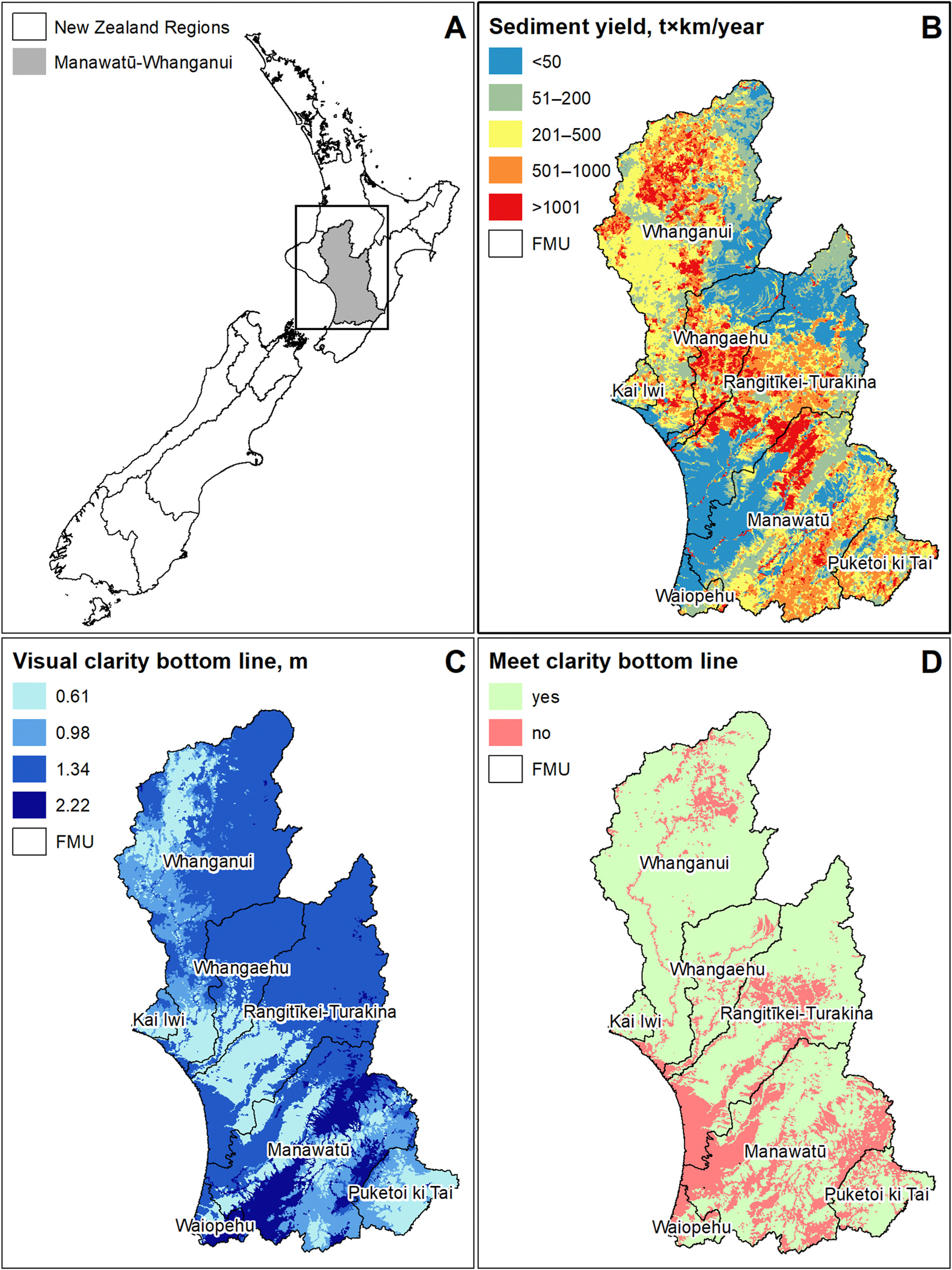
Manawatū-Whanganui Region: location map (panel A); sediment yields (panel B); national bottom line for water clarity (panel C); and watersheds that met national bottom line for water clarity in 2021 (Vale et al., 2022) (panel D).
The region has a diverse landscape, including mountain ranges and volcanic plateaus in the headwaters of the major rivers, dissected hill country, marine terraces, and alluvial plains in most of the middle reaches before flowing through coastal lowlands and sand dunes. The dominant geology in the region includes tertiary sandstone, mudstone, and siltstone varying in age from Jurassic/Triassic to present-day alluvial and marine deposits (Dymond et al., 2006; Heerdegen and Shepherd, 1992). Volcanic bedrock occurs in the central volcanic plateau surrounding the Tongariro and Ruapehu mountains and forms the headwaters of the Whanganui and Whangaehu rivers. The Tararua and Ruahine ranges are fault-bounded mountain ranges, rising to 1500 m with steep slopes and consisting of uplifted Torlesse Greywacke sandstone and argillite. These mountain ranges form an axial divide through the Manawatū catchment and serve as the catchment’s main headwaters (Vale et al., 2016, 2023). Steep hillslope terrain is common throughout the region, primarily underlain by soft mudstone which is prone to shallow landslides (Basher, 2013). Uplift and repeated downcutting have resulted in dissected hills and river terrace sequences, resulting in semi-confined channels through mudstone bedrock cliffs and alluvial terraces in much of the middle reaches of the major rivers (e.g. Manawatū, Whanganui, and Rangitīkei). Loess deposits are also common on top of many of the terraces and rolling land between the coastal sand country and inland hill country (Cowie, 1964). Extensive alluvial floodplains and coastal sand country occur in the lower reaches of the Manawatū.
The dominant soils in the region are Brown soils (particularly Orthic and Firm) according to the New Zealand Soil Classification (NZSC) after Hewitt (2010). These soils have a brown or yellow-brown subsoil below a relatively stable dark grey-brown topsoil. They are found throughout the hill country, typically where summer drought is uncommon, and are not waterlogged during winter. Pallic soils (including Perch-Gley, Immature, and Argillic) commonly derive from loess and greywacke parent material and tend to be dry in summer and wet in winter. Allophanic soils (including Allophanic brown) are mostly found in volcanic ash and from weathering products of other volcanic rocks in the northern part of the region. Gley soils are found throughout the lowland floodplains, where there are high ground-water tables and are often extensively drained (Hewitt, 2010).
The region’s climate is characterized by disturbed westerly airflow and anticyclones, modified by local topography, and generally has few climatic extremes, except in higher elevation areas (Chappell, 2015). The region has warm summers and mild winters, with annual rainfall between 800 and 1800 mm but reaching 5000 mm at higher altitudes (Dymond et al., 2006). Before human settlement, indigenous forests covered the hills and lowlands. Most of these forests were cleared for pastoral agriculture, which now covers 56% of the region. The other major land covers are indigenous forest (24%), scrub and shrubland (13%), and exotic forest (7%), with minor areas of cropland and other vegetation types (Basher et al., 2020). This deforestation accelerated erosion (Glade, 2003). The Manawatu-Whanganui region has the largest area of highly erodible land (as defined by Dymond et al. (2006); Page et al. (2005)) in New Zealand, accounting for 18% of the nation’s total highly erodible land despite comprising only 8.1% of its land area StatsNZ (2019). Additionally, it contains the largest area in the country with a high risk of landslides (StatsNZ, 2019).
2.2. Management of soil erosion in the region
Following the February 2004 storms (Hancox and Wright, 2005), Horizons Regional Council formed the Sustainable Land Use Initiative (SLUI) to reduce hill-country erosion and improve resilience to large storm events by developing whole-farm plans and implementing erosion control works (Manderson et al., 2013). The previously separate Whanganui Catchment Strategy, established before the SLUI, has been integrated into the programme. SLUI is informed by the Highly Erodible Land (HEL) model. The HEL model identifies highly erodible land using land cover, land use, soil, slope, and landslide risk (Dymond et al., 2006; Page et al., 2005).
Horizons Regional Council developed a classification system within the region that separates land into ‘top’, ‘high’, ‘low’, and ‘not’ priority. Top-priority land is estimated to contribute 40–55% of the sediment in the region’s rivers, and high-priority land contributes a further 25–30% of the sediment. By 2018, approximately 5000 km2 of land had whole farm plans. The main erosion mitigation measures were space-planting of trees, afforestation, retirement from grazing, and riparian retirement targeting highly erosion-prone land (Basher et al., 2020). As a result of the implementation of whole farm plans, it was estimated that the average annual sediment load reduced from 2004 to 2018 by 6.2%: from 13.4 Mt/yr in 2004 to 12.6 Mt/yr in 2018 (Basher et al., 2020).
The National Objectives Framework within the NPS-FM requires regional councils to set objectives for suspended fine sediment in their regions (NPS, 2020). Managing suspended fine sediment is a component of the NPS-FM, along with other contaminants such as nitrogen, phosphorus, and Escherichia coli, and visual clarity at measurement sites is used to determine outcomes.
Fig. 1B shows the modelled suspended sediment yield by River Environment Classification v2 (REC2) watersheds (i.e., each REC2 watershed drains to an individual segment of the REC2 digital stream network for the region). Fig. 1C shows the NBLWC for REC2 watersheds. There are 53,564 REC2 watersheds with an average area of 41 ha in the Manawatū-Whanganui Region. Fig. 1D shows REC2 watersheds where modelled water clarity met the NBLWC in 2021. Column 4 in Table 1 shows the proportion of waterways that met the NBLWC in 2021 by Freshwater Management Unit (FMU) and for the region. Column 5 in Table 1 shows the average weighted visual water clarity by FMU and for the region based on modelling by Fraser and Snelder (2020) and Vale et al. (2022).
Table 1.
Characteristics of freshwater management units in 2021.
| Freshwater Management Unit | Area, km2 | Length of waterways, km | Proportion of waterways that meet NBLWC | Average modelled water clarity, m |
|---|---|---|---|---|
|
| ||||
| Kai Iwi | 333 | 558 | 93.6% | 1.15 |
| Manawatū | 5,878 | 9,941 | 58.9% | 1.38 |
| Puketoi ki Tai | 1,168 | 1,825 | 67.8% | 0.92 |
| Rangitīkei-Turakina | 5,203 | 8,563 | 72.0% | 1.40 |
| Waiopehu | 394 | 647 | 53.9% | 1.61 |
| Whangaehu | 1,995 | 3,478 | 84.1% | 1.55 |
| Whanganui | 7,221 | 11,709 | 90.4% | 1.70 |
| Manawatū-Whanganui Region | 22,191 | 36,720 | 75.3% | 1.48 |
3. Materials and methods
The analysis encompasses key components outlined in Fig. 2, including data and assumptions (left) and models and output (right). First, we utilise the SedNetNZ model (Dymond et al., 2016) to forecast mean annual suspended sediment loads for two erosion mitigation scenarios spanning from 2021 to 2100. Second, we use the output of SedNetNZ to derive simplified relationships between mitigation actions and resulting changes in their outcomes (sediment loads and water clarity) that would be practical to use in a cost-benefit analysis. Next, we used these relationships and mitigation costs to calculate spatially explicit marginal costs to achieve water quality targets and improve water clarity. Finally, we developed marginal abatement cost curves. The following subsections describe these steps in detail.
Fig. 2.

Structure of the analysis.
3.1. Modelling soil erosion, sediment yield, and water quality
This analysis utilizes sediment modelling from the spatially explicit SedNetNZ sediment budget model applied in the Manawatū-Whanganui Region (Vale and Smith, 2023). SedNetNZ is a process-based erosion model that estimates the generation and transport of sediment through river networks (Dymond et al., 2016). SedNetNZ represents mean annual suspended sediment loads from hillslope (i.e., shallow landslide, earthflow, gully, and surficial erosion) and riverbank erosion processes (Dymond et al., 2016; Smith et al., 2019), while accounting for overbank floodplain deposition and sediment storage in lakes (Vale et al., 2022).
The SedNetNZ sediment budget model was developed to represent the range of erosion processes that occur in New Zealand (e.g., shallow landslides, earth flows, gully erosion, surficial erosion, and stream bank erosion), and includes parameterisation using erosion process data from New Zealand (e.g., Betts et al., 2017). This makes the model more suited to New Zealand’s diverse landscape and environmental management and planning needs compared to models like RUSLE (the Revised Universal Soil Loss Equation) or SWAT (Soil and Water Assessment Tool). For example, RUSLE represents a limited range of erosion processes (sheet and rill erosion), and SWAT (Soil and Water Assessment Tool) uses MUSLE (the Modified Universal Soil Loss Equation) to model hillslope erosion but does not include mass movement processes such as landslides, which is a significant erosion process in New Zealand, particularly in the Manawatū-Whanganui Region (Basher, 2013; Vale and Smith, 2023). Exclusion of these processes when they are important contributors to the catchment sediment budget, such as in New Zealand, can lead to an underestimation of sediment yields (Neverman et al., 2023).
The present study used SedNetNZ to model mean annual suspended sediment loads for two scenarios of on-farm erosion mitigation implementation and maturation of works across the Manawatū-Whanganui Region at 5-year intervals from 2021 to 2100. The five erosion mitigation measures considered in the analysis included afforestation, bush retirement, riparian retirement, space-planted trees, and gully tree planting. The application of these erosion mitigation works primarily occurs through the implementation of SLUI whole farm plans and the associated SLUI priority class (‘top’, ‘high’, ‘low’, and ‘not’ priority). Also, non-SLUI works (e.g., stream fencing and riparian planting in the lowland areas) occurring through other initiatives are also represented in the scenarios.
The first management scenario (PS1) included the maturation of existing SLUI/Whanganui Catchment Strategy works on farms with existing plans and future SLUI/Whanganui Catchment Strategy works continuing at the current rate. The second management scenario (PS2) included all whole farm plans implemented by 2030 and works on top-priority land implemented by 2035, on high-priority land by 2045, and on low-priority land by 2065. Non-SLUI works were modelled to reflect the full implementation of stock exclusion regulations by July 1, 2025 for both PS1 and PS2. The areas of erosion mitigation measures in each scenario are presented in Table 2. Full descriptions of the model scenarios can be found in Vale and Smith (2023).
Table 2.
Areas of erosion mitigation measures in modelling scenarios PS1 and PS2 and establishment cost for the Manawatū-Whanganui Region.
| Mitigation measures (k) | PS1, area, ha | PS2, area, ha | Establishment Cost, $/ha |
|---|---|---|---|
|
| |||
| Afforestation (forestry-conifer) | 107,816 | 137,438 | 1,700 |
| Bush retirement (reversion-retirement) | 73,799 | 89,825 | 950 |
| Riparian retirement (reversion-riparian) | 9,029 | 10,031 | 3,200 |
| Space-planted trees | 46,087 | 55,028 | 875 |
| Gully tree planting (forestry-conifer) | 1,239 | 1,575 | 1,700 |
3.2. Relationships between mitigation measures and policy-relevant outcomes
SedNetNZ (Dymond et al., 2016) is a complex model that uses multiple parameters to capture the influence of land use on soil erosion and sedimentation. Consequently, it is not feasible to explicitly integrate the biophysical process model into a cost-effectiveness analysis or a cost-benefit analysis tool. Therefore, our aim is to derive simplified relationships between mitigation actions and their outcomes that would be practical to use in a cost-benefit analysis. Specifically, we estimate the marginal costs of achieving the specific NBLWC in each stream segment and the marginal cost of improving the average water clarity across the region’s stream network.
We use outputs from the latest SedNetNZ modelling for the region (Vale and Smith, 2023) and multiple regressions to derive relationships between the areas of mitigation measures, the baseline sediment load for watersheds draining to each stream segment, the changes in the length of the stream network that meet the NBLWC, and the changes in average water clarity. Modelled changes in water clarity in any segment of the stream network depend on mitigations in all watersheds upstream. Therefore, changes in clarity related to mitigations can only be modelled at the catchment level (i.e., comprising multiple segment-level watersheds) or further aggregated into FMUs that are used by the regional council, which combine several catchments draining to the sea.
We find that there is insufficient variability within catchments or FMUs to model water clarity as a function of the five mitigation measures (and other factors) using multiple regression. Therefore, we undertake a two-step process. In step one, we estimate the relationship between the mitigation measures and changes in sediment load at the REC2 watershed level. In step two, we estimate the FMU-level relationship between the changes in sediment load and changes in the length of the stream network that meets the NBLWC and the relationship between sediment yield and the changes in average clarity.
Spatial dependencies between observations are likely because of unobservable or omitted factors such as soil, precipitation, land cover, and spatially correlated explanatory variables. Using Ordinary Least Squares in such circumstances may lead to biased parameter estimates and invalid standard errors. Common approaches to deal with these issues are spatial fixed effect models, spatial heteroskedasticity and autocorrelation consistent (spatial HAC) estimators, and spatial estimators (spatial error and/or lag models). In the REC2-level regression, we use Conley Spatial HAC estimators (Conley, 1999).
First, we estimate the linear relationship between the mitigation measures and the modelled changes in sediment load and clarity. Maturation (or time between the implementation and effectiveness of mitigation measures) takes 2–15 years. Therefore, we assume that mitigation measures implemented during a 10-year period are related to changes in sediment load in the next 10-year period:
| (1) |
where is the change in average annual sediment load generated by the REC2 watershed in a scenario during a 10-year (decadal) period is the area (ha) of mitigation measure implemented in this watershed during the previous 10-year period is the sediment yield in the watershed before the implementation of the measures; are regression parameters to be estimated; and is the residual.
The model is estimated without an intercept because we assume all the modelled change in sediment load is attributed to mitigation measures. Including the intercept would mean there are changes in the sediment load of water clarity without any mitigation works, which is not plausible in this context.
Second, we estimate the linear relationship between changes in the gross sediment load (not accounting for the deposition of sediments) and changes in the length of streams that meet the NBLWC at an FMU level:
| (2) |
where is the change in the length of streams that meets the NBLWC in the FMU , scenario and a 10-year period is the change in gross annual sediment load generated by all the REC2 watersheds within FMU during a 10-year period is the regression coefficient to be estimated; and is the residual.
To estimate the relationship between changes in the sediment load and changes in water clarity, we calculated the water clarity for each REC2 in future periods based on the equation by Hicks et al. (2019):
where is the clarity in REC2 segment in year is the clarity in the base year (2021) from Vale et al. (2022); and are sediment loads in REC2 segment in the base year and year from Vale et al. (2022); and is −0.76 (Hicks et al., 2019).
The average changes in water clarity for every decade and scenario in each FMU were calculated as length-weighted averages of all REC2 segments in a catchment:
where is the change in water clarity in REC2 segment is the change in water clarity in FMU and scenario during a decade ; and is the length of the REC2 segment in FMU .
For consistency, we related the changes in average water clarity to changes in average gross sediment yields, calculated as summed changes in sediment loads divided by the summed areas of REC2 segments in each FMU:
where is the change in average gross sediment yields in FMU , scenario , and decade ; and is the area of REC2 watershed in an FMU .
We estimate the linear relationship between changes in sediment yield and changes in the average water clarity by catchment as:
| (3) |
where is the regression coefficient to be estimated, and is the residual.
3.3. Cost-effectiveness
We modelled the cost of mitigation measures as the sum of initial capital (establishment) cost and annual opportunity cost. The cost of establishing mitigation measures was obtained from Horizons Regional Council’s Hill Country Erosion Programme 2019–2023 application (Table 2). Maintenance costs were not separately included into our calculations. Short-term maintenance costs are factored in establishment costs, while long-term ongoing maintenance costs are uncertain. To address this we used a wide range of variation in establishment costs during sensitivity analysis. The opportunity costs were calculated by capitalizing the net revenue, measured as earnings before interest and taxes (EBIT) of land uses for the Manawatū-Whanganui Region (Table 3) from the New Zealand Forest and Agriculture Regional Model (Daigneault et al., 2018; Greenhalgh and Djanibekov, 2022) at a 5% interest rate. The EBIT for each REC2 polygon was calculated as the area-weighted average of the EBIT of the different land uses in each watershed. We assumed there are no opportunity costs for gully tree planting and for space-planted trees because gullies are not used in agricultural production, and the pastures with space-planted trees are not excluded from grazing.
Table 3.
Earnings before interest and taxes (EBIT) of land uses for the Manawatū-Whanganui Region.
| Land use | Area, ha | Mean EBIT, $/ha/yr |
|---|---|---|
|
| ||
| Arable | 6,229 | 1,650 |
| Dairy | 234,247 | 1,686 |
| Exotic forestry on farm | 266,625 | 273 |
| Fruit | 924 | 7,406 |
| Sheep, beef, and deer | 935,949 | 226 |
| Vegetables | 1,465 | 9,356 |
After estimating the regression models (1–3), we can calculate the marginal cost of achieving NBLWC and reduction of average clarity as:
| (4) |
| (5) |
where is the marginal cost of achieving the NBLWC (i.e., the cost of achieving the NBLWC in an additional meter of stream) from implementing mitigation measure in REC2 watershed is the marginal cost of improving average water clarity in the region (i.e., the cost of increasing the average weighted water clarity by an additional meter) by implementing mitigation measure in REC watershed is the opportunity cost of land use in REC2 watershed is the establishment cost of mitigation action is the sediment yield in REC2 watershed is the area of the region; and , and are the regression coefficients.
3.4. Marginal abatement cost curves
The cost-effectiveness of pollution reductions ordered and mapped out on a chart is known as a marginal abatement cost curve (Kesicki and Strachan, 2011; McKitrick, 1999). A marginal abatement cost curve (MACC) is widely used to analyse options for greenhouse gas mitigation and its costs (Morris et al., 2012), but also for analysing the abatement of water pollution (Hou et al., 2015; Marinoni and van Grieken, 2016). We developed MACCs for achieving NBLWC and improving region-average water clarity using marginal costs and mitigable areas from the PS2 scenario in Vale and Smith (2023).
4. Results
4.1. Results of modelling soil erosion, sediment yield, and water quality
We employed the SedNetNZ model to forecast mean annual suspended sediment loads across the Manawatū-Whanganui Region from 2021 to 2100 under two distinct erosion mitigation scenarios. We derived two datasets from the model outputs for regression analysis. The first dataset contains data by REC2 watershed and decade and includes base-level sediment yield, the spatial extent of mitigation measures over 10-year intervals, and the lagged 10-year changes in annual sediment load. The second dataset is aggregated by the Freshwater Management Unit (FMU) and decade and includes changes over 10-year periods in various parameters, including the length of waterways meeting water quality standards, average weighted water clarity, gross sediment load, and sediment yield. Detailed descriptive statistics of these variables are provided in Table 4.
Table 4.
Descriptive statistics.
| Variables | Mean | SD | Min | Max |
|---|---|---|---|---|
|
| ||||
| By REC2 watershed (n = 588,467) | ||||
| Change in sediment load, t/yr | 13.52 | 38.89 | 0.00 | 1,776.09 |
| Sediment yield, t/km2/yr | 417.31 | 629.37 | 0.00 | 50,470.12 |
| Area of afforestation, ha | 0.38 | 0.86 | 0.00 | 23.36 |
| Area of retirement, ha | 0.26 | 0.62 | 0.00 | 18.53 |
| Area of gully planting, ha | 0.004 | 0.05 | 0.00 | 7.94 |
| Area of riparian retirement, ha | 0.029 | 0.21 | 0.00 | 13.96 |
| Area of space-planted trees, ha | 0.15 | 0.36 | 0.00 | 10.19 |
| By FMU and decade (n = 98) | ||||
| Change in length of waterways that meet NBLWC, m | 76,977.32 | 124,913.47 | 0.00 | 722,601.31 |
| Change in average clarity, m | 0.10 | 0.12 | 0.00 | 0.66 |
| Change in gross sediment load, t/yr | 81,725.52 | 113,914.99 | 14.85 | 505,027.79 |
| Change in sediment yield, t/km2/yr | 23.40 | 26.51 | 0.04 | 129.69 |
| Area, km2 | 3,170.22 | 2,659.91 | 332.80 | 7,221.22 |
4.2. Relationships between mitigation measures and policy-relevant outcomes
The results of estimating Model (1) are presented in Table 5. Due to the correlation between the area of afforestation and the area of bush retirement in the modelling and because their impact is assumed to be identical (Vale and Smith, 2023), we combined these two variables. The coefficients are statistically significant and meaningful and vary across mitigation measures.
Table 5.
Regression results of the relationship between the mitigation measures and changes in sediment load at the REC2 watershed level.
| Variable | Dependent variable: change in sediment load |
|---|---|
|
| |
| Area of afforestation and retirement × sediment yield | 0.017*** (0.001) |
| Area of gully planting × sediment yield | 0.042*** (0.014) |
| Area of riparian retirement × sediment yield | 0.029*** (0.011) |
| Area of space-planted trees × sediment yield | 0.027*** (0.003) |
| Number of observations | 588,467 |
| R2 | 0.779 |
| Standard errors | Conley Spatial HAC (20 km) |
p < 0.1,
p < 0.05,
p < 0.01.
The results of estimating Model (2) are presented in Table 6. Two FMU-specific coefficients are not statistically significant. These are the smallest FMUs in the region (Kai Iwi and Waiopehu) (see Fig. 1 and Table 1). Small values of the coefficients are for the FMUs with a large proportion of the stream network that meets the NBLWC (Kai Iwi and Whanganui), and large values of the coefficients are for the FMUs with the lowest proportions of streams that meet the NBLWC (Manawatū and Waiopehu). This is because reducing sediment load in FMUs with the lowest proportion of the stream network meeting the NBLWC would improve the water clarity. According to the law of diminishing returns, after a certain point (i.e., after some level of investment in something), even if you continue investing in it (in this case, erosion mitigation measures), the return gets lower and lower.
Table 6.
Regression results from the relationship between the changes in sediment load and change in the length of streams that meet the NBLWC at the catchment level.
| Variable | Dependent variable: change in length of waterways that meet the NBLWC |
|---|---|
|
| |
| Gross sediment load × FMU Kai Iwi | 0.367 (1.607) |
| Gross sediment load × FMU Manawatū | 1.348*** (0.056) |
| Gross sediment load × FMU Puketoi ki Tai | 1.394*** (0.221) |
| Gross sediment load × FMU Rangitīkei-Turakina | 0.977*** (0.058) |
| Gross sediment load × FMU Waiopehu | 3.283 (14.821) |
| Gross sediment load × FMU Whangaehu | 0.512*** (0.107) |
| Gross sediment load × FMU Whanganui | 0.637*** (0.055) |
| Number of observations | 98 |
| R2 | 0.921 |
p < 0.1,
p < 0.05,
p < 0.01.
The results of estimating Model (3) are presented in Table 7. All FMU-specific coefficients are statistically significant (except Waiopehu, which is a small FMU) and meaningful.
Table 7.
Regression results from the relationship between sediment yield changes and the average water clarity change.
| Variable | Dependent variable: change in average clarity |
|---|---|
|
| |
| Sediment yield × FMU Kai Iwi | 0.00365*** (0.00095) |
| Sediment yield × FMU Manawatū | 0.00381*** (0.00058) |
| Sediment yield × FMU Puketoi ki Tai | 0.00380*** (0.00046) |
| Sediment yield × FMU Rangitīkei-Turakina | 0.00415*** (0.00054) |
| Sediment yield × FMU Waiopehu | 0.00681 (0.01042) |
| Sediment yield × FMU Whangaehu | 0.00400*** (0.00038) |
| Sediment yield × FMU Whanganui | 0.00387*** (0.00071) |
| Number of observations | 98 |
| R2 | 0.782 |
p < 0.1,
p < 0.05,
p < 0.01.
4.3. Cost-effectiveness
The marginal costs of achieving NBLWC and improving the average water clarity of streams (equations (4) and (5)) depend on the sediment yields and opportunity costs in REC2 watersheds. Both of these factors vary significantly across the region. To compare the values and demonstrate the distribution of marginal costs, we use sediment yields and opportunity costs in mitigable areas of the region. We use REC2 watersheds where mitigation measures were implemented in scenario PS2 (Vale and Smith, 2023) between 2021 and 2100. We also use areas of the mitigation measures in each REC2 watershed as weights to calculate the distributions.
We present the means and the distributions of costs, yields, and marginal costs in Table 8. Panel A of Table 8 shows the means, variations, and ranges of costs (establishment cost plus opportunity cost) for each mitigation measure. The differences between the costs of mitigation measures are driven by the differences in establishment costs and opportunity costs that depend on land uses (and location). There is no variation in the costs of space-planted trees and gully tree planting because they do not include opportunity costs. Riparian retirement has the highest costs due to being implemented in flatter, more productive areas with higher opportunity costs.
Table 8.
Distribution of (A) costs of mitigation measures ($/ha), (B) sediment yield (t/ha/yr), (C) inverse sediment yield (ha/t/yr), (D) marginal costs of achieving NBLWC ($/m), and (E) marginal costs of improving region-average water clarity ($million/m) in REC2 watersheds where erosion mitigation measures are implemented during 2021–2100 according to scenario PS2.
| Mitigation measure | Mean | STD | CV | P05 | Q1 | Median | Q3 | P95 |
|---|---|---|---|---|---|---|---|---|
|
| ||||||||
| (A) Costs of mitigation measures ($/ha) | ||||||||
| Afforestation | 7,180 | 4,155 | 0.58 | 6218 | 6218 | 6366 | 6596 | 7534 |
| Gully tree planting | 1,650 | 0 | 0.00 | 1650 | 1650 | 1650 | 1650 | 1650 |
| Bush retirement | 6289 | 3,723 | 0.59 | 5468 | 5468 | 5635 | 5851 | 6320 |
| Riparian retirement | 11,397 | 11,369 | 1.00 | 7718 | 7718 | 7944 | 8162 | 36,300 |
| Space-planted trees | 875 | 0 | 0.00 | 875 | 875 | 875 | 875 | 875 |
| (B) Sediment yield (t/ha/yr) | ||||||||
| Afforestation | 748 | 532 | 0.71 | 106 | 407 | 669 | 968 | 1604 |
| Gully tree planting | 1,728 | 986 | 0.57 | 160 | 891 | 1727 | 2640 | 3167 |
| Bush retirement | 780 | 544 | 0.70 | 125 | 436 | 703 | 1003 | 1694 |
| Riparian retirement | 146 | 399 | 2.74 | 1 | 10 | 53 | 176 | 527 |
| Space-planted trees | 706 | 539 | 0.76 | 95 | 373 | 606 | 894 | 1656 |
| (C) Inverse sediment yield (ha/t/yr) | ||||||||
| Afforestation | 0.0040 | 0.0167 | 4.22 | 0.0006 | 0.0010 | 0.0015 | 0.0025 | 0.0095 |
| Gully tree planting | 0.0019 | 0.0069 | 3.63 | 0.0003 | 0.0004 | 0.0006 | 0.0011 | 0.0063 |
| Bush retirement | 0.0035 | 0.0150 | 4.26 | 0.0006 | 0.0010 | 0.0014 | 0.0023 | 0.0080 |
| Riparian retirement | 0.2301 | 0.8220 | 3.57 | 0.0019 | 0.0057 | 0.0190 | 0.1047 | 0.8333 |
| Space-planted trees | 0.0042 | 0.0166 | 3.99 | 0.0006 | 0.0011 | 0.0017 | 0.0027 | 0.0106 |
| (D) Marginal costs of achieving NBLWC ($/m) | ||||||||
| Afforestation | 2178 | 18,162 | 8.34 | 246 | 453 | 660 | 1162 | 5431 |
| Gully tree planting | 102 | 418 | 4.11 | 10 | 14 | 23 | 50 | 386 |
| Bush retirement | 1708 | 15,091 | 8.84 | 203 | 391 | 569 | 954 | 4,015 |
| Riparian retirement | 142,738 | 827,365 | 5.80 | 583 | 2,110 | 4,967 | 43,191 | 505,228 |
| Space-planted trees | 157 | 733 | 4.67 | 19 | 39 | 59 | 104 | 373 |
| (E) Marginal costs of improving region-average water clarity ($million/m) | ||||||||
| Afforestation | 10,704 | 66,220 | 6.19 | 1,364 | 2,173 | 3159 | 5,411 | 28,066 |
| Gully tree planting | 432 | 1,573 | 3.64 | 69 | 85 | 132 | 249 | 1,427 |
| Bush retirement | 8,376 | 55,026 | 6.57 | 1,144 | 1,855 | 2650 | 4429 | 20,455 |
| Riparian retirement | 878,262 | 5,220,360 | 5.94 | 3,193 | 8,983 | 30,688 | 219,723 | 2,579,772 |
| Space-planted trees | 761 | 2,986 | 3.92 | 111 | 204 | 305 | 498 | 1,959 |
Notes: CV is the coefficient of variation, P05 and P95 are the 5th and 95th percentiles, and Q1 and Q3 are the 1st and 3rd quartiles.
Panel B of Table 8 presents the means, variations, and ranges of sediment yield by mitigation measure. Because sediment yield enters cost-effectiveness in the denominator (equations. (4) and (5)), we also show the variation of inverse sediment yield (panel C in Table 8). There is a wide variation in sediment yields (as indicated by the coefficient of variation, CV) but even greater variations in inverse sediment yields in REC2 watersheds where each mitigation measure was implemented in scenario PS2. However, riparian retirement was planned and implemented in the REC2 watersheds with the lowest sediment yields, while gully tree planting was implemented in the REC2 watersheds with the highest sediment yields. This has implications for cost-effectiveness, as the effectiveness of all mitigation measures increases with the increase in sediment yield.
We present the means, variation, and distributions of marginal costs of achieving NBLWCs, and of the marginal costs of improving region-average water clarity, in Panels D and E (respectively) of Table 8. Both marginal costs substantially vary because they depend on the baseline sediment load and opportunity costs, which are also correlated. Comparing the coefficients of variations of costs, inverse sediment yields, and marginal costs indicates that most of the variation in the marginal costs is due to variation in sediment yields across the landscape. The lowest marginal costs of both achieving NBLWCs and improving water clarity are for gully tree planting and space-planted trees, partly because of no opportunity costs. The highest marginal costs are for riparian retirement because the mitigation measure is primarily implemented in areas with the lowest sediment yield, on more productive lands (therefore with the highest opportunity costs), and because of the highest establishment costs.
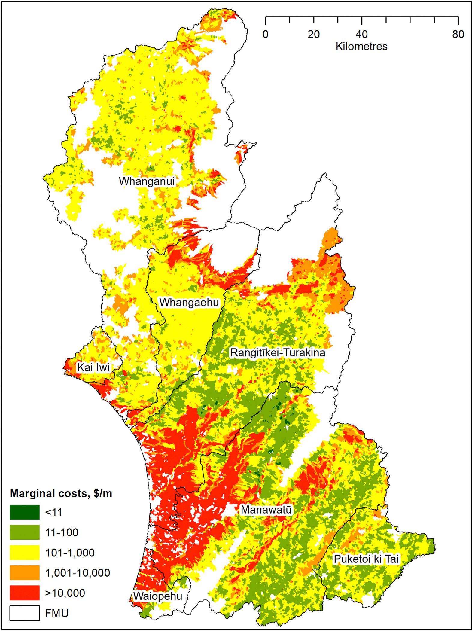
The spatial distributions of marginal costs of achieving NBLWCs by mitigation measure are presented in Fig. 3. In addition, Fig. 4 shows the REC2-level average weighted marginal costs of achieving NBLWC based on a mix of mitigation measures implemented in the PS2 scenario (Vale and Smith, 2023) in each REC2 watershed.
Fig. 3.

The spatial distribution of the marginal cost of achieving the national bottom line for water clarity ($/m) in the Manawatu-Whanganui region, by mitigation measure. The marginal costs are shown only for REC2 watersheds where gully tree planting, afforestation, space planting, bush retirement, and riparian retirement were modelled by Vale and Smith (2023).
Fig. 4.
The spatial distribution of the weighted average marginal cost of achieving the national bottom line for water clarity ($/m), by REC2 watersheds where gully tree planting, afforestation, space-planting, bush retirement, and riparian retirement were modelled by Vale and Smith (2023).
4.4. Marginal abatement cost curves
Fig. 5 shows MACCs for achieving NBLWC. For mitigable areas in each REC2, we estimated marginal costs, total costs, and changes in the length of the stream network that meet the NBLWC as a result of the implementation of mitigation works. We ordered all mitigable areas by marginal costs and grouped them into bins, each representing an increase in the length of stream meeting the NBLWC by 1%. The x-axis is the percentage of the stream network of the region that meets NBLWC, and the y-axis is the cost of achieving 1% of the NBLWC target.
Fig. 5.
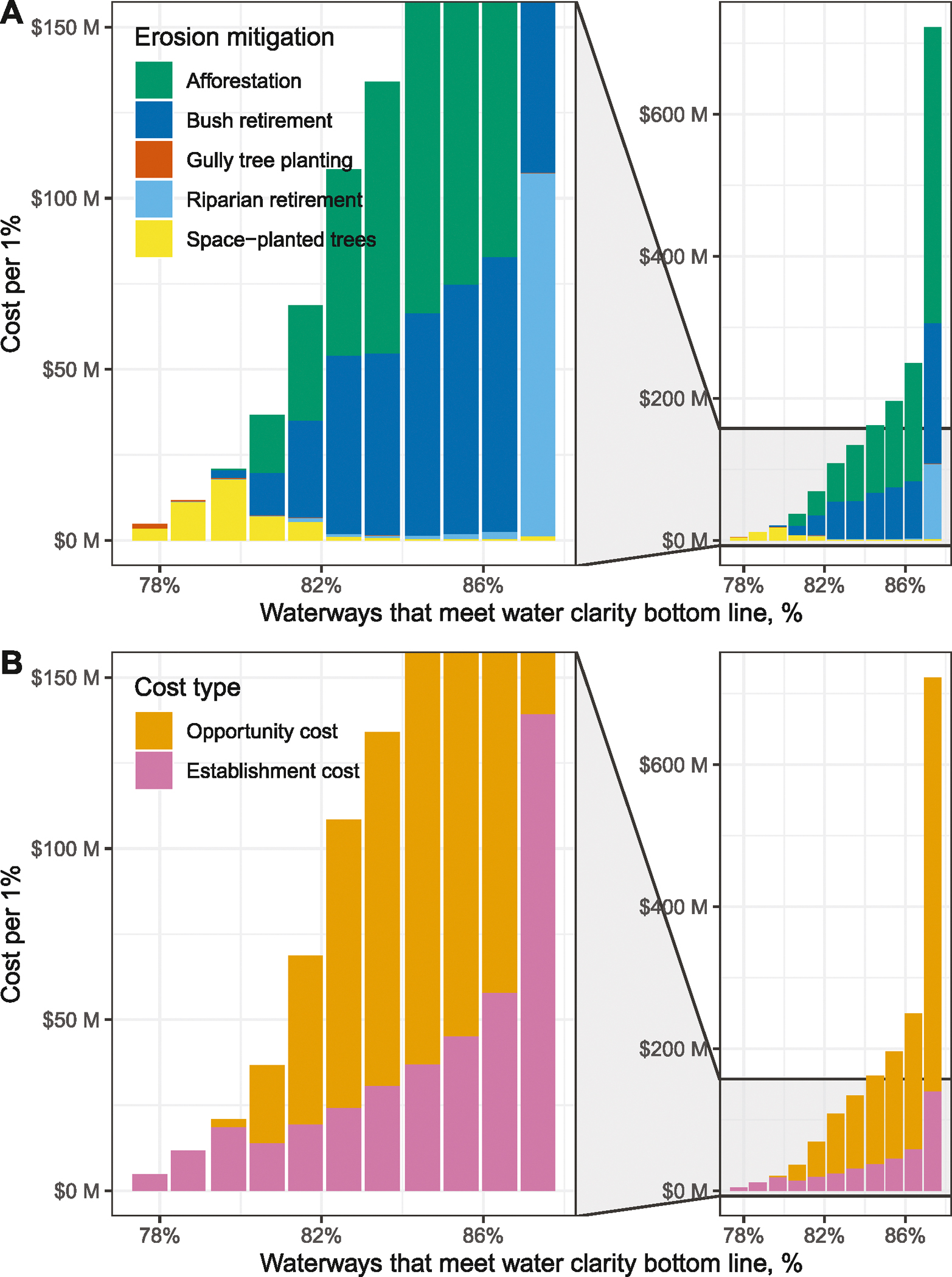
The marginal abatement costs curve of achieving national bottom line for water clarity, with breakdown by mitigation measures (afforestation, bush retirement, gully tree planting, riparian retirement, and space-planted trees) (panel A) and by type of costs (establishment and opportunity) (panel B).
Fig. 5A shows the costs broken down by mitigation works, and Fig. 5B shows the breakdown by establishment and opportunity costs. The resulting graph forms an MACC. The marginal cost of achieving NBLWC increases nearly exponentially, which is typical for water quality abatement costs (Polyakov and White, 2022; Roberts et al., 2012). When prioritised by cost-effectiveness, the mitigation works are ranked as follows: gully tree planting, space-planted trees, afforestation, bush retirement, and, finally, riparian retirement (Fig. 5A). As costs increase, the proportion of opportunity costs rises (Fig. 5B).
Fig. 6 shows MACCs for improving region-average water clarity. The mitigable areas were ordered by marginal costs of improving water clarity and grouped by bins representing a 5 cm improvement in average water clarity, broken down by mitigation measure (Fig. 6A) and cost component (Fig. 6B). The shape of the resulting MACC is similar to that of the MACC for achieving NBLWC. In this case, the marginal costs can be compared with the willingness to pay for the improvement of water clarity. Walsh et al. (2023) estimated region-specific willingness to pay for water quality attributes, including water clarity. The willingness to pay (WTP) for water quality in the Manawatū-Whanganui region is estimated at $135.19/m/household/yr (90% confidence interval 42.21, 228.17), equivalent to $6.75/5 cm/household/yr. The WTP of the population of the Manawatu-Wanganui Region (90,408 households in 2018) for improvement in average water clarity by 5 cm is $611,000/yr. When capitalized at 5% to be comparable with the cost, the Manawatu-Wanganui WTP is $12.2 million/5 cm (black line in Fig. 6). Applying a marginal cost equal to the marginal benefits optimality condition and ignoring co-benefits of mitigation measures, the optimal level of mitigation is where it achieves approximately 15 cm improvement of average water clarity.
Fig. 6.

The marginal abatement costs curve of improving region-average water clarity with the breakdown by mitigation measure (afforestation, bush retirement, gully tree planting, riparian retirement, and space-planted trees) (panel A) and by type of costs (establishment costs and opportunity costs) (panel B).
4.5. Sensitivity analysis
To test the stability of this optimal level of mitigation, we conducted a sensitivity analysis by varying discount rate (2% and 8%), WTP (lower and upper bound of 90% confidence interval), establishment costs (+50%, +25%, and −25%) and opportunity costs (+25%, −25%, and no opportunity costs). We also estimated the optimal level of mitigation for a scenario where afforestation generates annualized EBIT benefits from harvesting (but not including carbon credits) equal to $273/yr (Ministry for Primary Industries, 2022). This last assumption differs from our baseline estimate that afforestation would not produce any revenue and thus have a higher opportunity cost, while, in reality, some afforested blocks might be large enough to produce merchantable timber that could be profitably harvested (Fernandez and Daigneault, 2017). Furthermore, this option may also come with increased sediment yield post-harvest due to increased erosion susceptibility for several years after harvesting.
For each alternative scenario, we estimated the improvement in water clarity where marginal costs equal marginal benefits and presented the optimal level of mitigation, total costs, and areas of mitigation works required to achieve this level (Table 9). The base scenario results in an ‘optimal’ (i.e., where MB = MC) set of mitigation measures being implemented on 20,929 ha, resulting in a 0.134 m improvement in water clarity with a capitalized cost of $19.19 million. Most mitigation measures are spaced tree (94%) and gully (6%) planting, as shown in Fig. 6 and consistent with the maps in Fig. 3.
Table 9.
Sensitivity analysis of the optimal allocation of erosion mitigation measures.
| Scenario: parameter to vary | Change in water clarity, m | Capitalized total costs, $M | Area of mitigation measures, ha |
||||||
|---|---|---|---|---|---|---|---|---|---|
| Afforestation | Gully tree planting | Bush retirement | Riparian retirement | Spaced tree planting | Total | ||||
|
| |||||||||
| Base case | N/A | 0.134 | 19.19 | 0 | 1170 | 0 | 7 | 19,652 | 20,829 |
| Interest rate | High (8%) | 0.067 | 6.29 | 0 | 898 | 0 | 3 | 5477 | 6379 |
| Low (2%) | 0.197 | 41.31 | 0 | 1374 | 0 | 10 | 44,442 | 45,826 | |
| WTP | UB 90% CI | 0.183 | 34.42 | 1 | 1328 | 2 | 13 | 36,693 | 38,037 |
| LB 90% CI | 0.025 | 1.63 | 0 | 208 | 0 | 0 | 1469 | 1677 | |
| Establishment cost | Very High (+50%) | 0.076 | 11.48 | 0 | 951 | 0 | 3 | 6924 | 7879 |
| High (+25%) | 0.103 | 15.58 | 0 | 1062 | 0 | 4 | 12,207 | 13,273 | |
| Low (−25%) | 0.165 | 21.04 | 0 | 1263 | 0 | 8 | 29,592 | 30,864 | |
| Opportunity cost | High (+25%) | 0.133 | 19.16 | 0 | 1170 | 0 | 3 | 19,652 | 20,826 |
| Low (−25%) | 0.134 | 19.19 | 0 | 1170 | 0 | 9 | 19,652 | 20,832 | |
| None | 0.221 | 33.99 | 3873 | 1170 | 8567 | 43 | 19,652 | 33,305 | |
| Timber benefit | Included | 0.204 | 21.53 | 11,836 | 1575 | 0 | 7 | 19,652 | 33,070 |
| All mitigable areas in PS2 scenario (Vale and Smith, 2023) | 0.71 | 1716 | 137,438 | 1575 | 89,825 | 9944 | 55,028 | 293,810 | |
The ‘optimal’ improvement in water clarity varies for different scenarios, ranging from 2.4 cm for a scenario with lower bound of the WTP 90% confidence interval to 22.1 cm for a scenario without opportunity costs. Gully tree planting and space-planted trees are dominant mitigation measures in most scenarios. In scenarios with no opportunity costs (i.e., no assumed loss in EBIT associated with any of the measures), afforestation and bush retirement are also included, and the total implementation area increases by 59% over the base case. When forestry EBIT benefits are included, afforestation becomes a cost-efficient mitigation option, comprising about one-third of the total mitigation area. For comparison, implementation of mitigation in all mitigable areas according to scenario PS2 in Vale and Smith (2023) would result in a 74.1 cm improvement in the region-average water clarity at a total capitalized cost of $1716 million.
5. Discussion and conclusions
New Zealand faces a significant erosion problem, and efforts are underway to manage erosion with new methods and policies. Given constrained budgets, it is essential to consider both the costs and the benefits of erosion mitigation in order to allocate limited resources efficiently to address the problem. In this study, we demonstrate a method for estimating the cost-effectiveness of erosion mitigation measures for achieving water clarity targets. Previous studies have estimated the cost-effectiveness of soil erosion reduction mitigation measures to reduce soil erosion (Girona-García et al., 2023; Jin and England, 2009; Ricci et al., 2020). However, government policies may target other metrics associated with erosion mitigation, such as water quality indicators measured at a catchment or regional scale. Estimates of the cost-effectiveness of erosion mitigation for achieving water clarity facilitate better targeting of investments in erosion mitigation.
Our findings show that cost-effectiveness has a substantial variation (coefficient of variation 3–6) and depends on multiple factors, such as type of mitigation and land-use profitability, but most of all, the sediment yield where the mitigation measures are implemented. Conditional on where each mitigation action is implemented in the landscape, the most cost-effective options for our study site are gully tree planting and spaced-tree planting, while the least cost-effective is riparian retirement. We developed marginal abatement cost curves to achieve the NBLWC and improve water clarity. These curves are commonly used in greenhouse gas mitigation literature and in analysing the abatement of water pollution (Marinoni and van Grieken, 2016). However, they have not been developed for soil erosion mitigation. These curves confirm the variability of marginal costs and show that marginal costs increase nearly exponentially, similar to water quality marginal abatement costs (Roberts et al., 2012).
No monetary estimate of the value of achieving the water clarity targets exists, so we estimated a cost-effective level of erosion mitigation using the willingness to pay for the increase in region-average water clarity. Based on the estimate that the average household in our study region would be willing to pay $1.35/cm/yr, an optimal approach would be to implement 21,000 ha of spaced-tree and gully tree planting at a cost of $19 million, or about $920/ha. Following this cost-effective approach would achieve a 13 cm improvement in the region’s average water clarity.
Our modelling approach did not account for improvements in other water quality attributes (e.g., nutrients and E. coli) that are likely to coincide with the adoption of erosion mitigation measures. Further, we do not include other environmental co-benefits of mitigation actions, such as carbon sequestration, biodiversity, and visual amenity. Accounting for these benefits would be likely to increase the optimal level of erosion mitigation and increase the cost-effectiveness of some mitigation measures, such as afforestation (for carbon sequestration) and riparian retirement (for E. coli and nutrient mitigation). For example, (Daigneault et al., 2017) conducted a benefit-cost analysis of riparian restoration in New Zealand that accounted for impacts on greenhouse gases, nutrients, and sediment and found that sediment accounted for less than 20% of the total monetized benefits.
These results are specific to the study region but may be applied to other areas of New Zealand and internationally where equivalent spatial erosion and sediment load modelling are available. Furthermore, the method may be extended to the cost-effectiveness of improving other policy-relevant water quality attributes, such as nutrients or E. coli concentrations. This spatially explicit analysis can help identify trade-offs in a cost-benefit decision framework if widely used. The estimates depend on existing research on productivity impacts and the quality of erosion and land-use data. These findings can also be combined with other cost-benefit estimates; for example, the non-market values of water quality benefits and the effect of soil erosion on agricultural productivity.
Acknowledgements
We thank participants of the 2023 AARES conference for helpful comments on an earlier version of this article. The work has been supported by funding from the Ministry of Business, Innovation and Employment programme Smarter Targeting of Erosion Control (contract CO9X1804).
Footnotes
Declaration of competing interest
The authors declare that they have no known competing financial interests or personal relationships that could have appeared to influence the work reported in this paper.
CRediT authorship contribution statement
Maksym Polyakov: Writing – original draft, Methodology, Formal analysis, Data curation. Patrick Walsh: Methodology, Conceptualization. Adam Daigneault: Writing – review & editing, Methodology, Formal analysis. Simon Vale: Writing – review & editing, Resources, Formal analysis, Data curation. Chris Phillips: Writing – review & editing, Project administration, Investigation, Funding acquisition, Conceptualization. Hugh Smith: Writing – review & editing, Supervision, Methodology, Conceptualization.
Data availability
The authors do not have permission to share data.
References
- Australian Government, 2018. Charter: National Water Quality Management Strategy. Department of Agriculture and Water Resources, Canberra. [Google Scholar]
- Barry LE, Paragahawewa UH, Yao RT, Turner JA, 2011. Valuing avoided soil erosion by considering private and public net benefits. In: New Zealand Agriculture and Resource Economics Society Conference. Nelson, New Zealand. [Google Scholar]
- Barry LE, Yao RT, Harrison DR, Paragahawewa UH, Pannell DJ, 2014. Enhancing ecosystem services through afforestation: how policy can help. Land Use Pol. 39, 135–145. [Google Scholar]
- Basher L, Djanibekov U, Soliman T, Walsh PJ, 2019. Literature Review and Feasibility Study for National Modelling of Sediment Attribute Impacts. Report prepared for Ministry for the Environment. [Google Scholar]
- Basher L, Spiekermann R, Dymond J, Herzig A, Hayman E, Ausseil A-G, 2020. Modelling the effect of land management interventions and climate change on sediment loads in the Manawatū–Whanganui region. N. Z. J. Mar. Freshw. Res. 54, 490–511. [Google Scholar]
- Basher LR, 2013. Erosion processes and their control in New Zealand. Ecosystem services in New Zealand–conditions and trends 2013, 363–374. [Google Scholar]
- Betts H, Basher L, Dymond J, Herzig A, Marden M, Phillips C, 2017. Development of a landslide component for a sediment budget model. Environ. Model. Software 92, 28–39. [Google Scholar]
- Beverly C, Roberts A, Doole G, Park G, Bennett FR, 2016. Assessing the net benefits of achieving water quality targets using a bio-economic model. Environ. Model. Software 85, 229–245. [Google Scholar]
- Blaschke P, Hicks D, Meister A, 2008. Quantification of the Flood and Erosion Reduction Benefits, and Costs, of Climate Change Mitigation Measures in New Zealand. Ministry for the Environment, Wellington. [Google Scholar]
- Bryan BA, Crossman ND, 2008. Systematic regional planning for multiple objective natural resource management. J. Environ. Manag. 88, 1175–1189. [DOI] [PubMed] [Google Scholar]
- Chappell PR, 2015. The Climate and Weather of Manawatu-Wanganui. NIWA. [Google Scholar]
- Conley TG, 1999. GMM estimation with cross sectional dependence. J. Econom. 92, 1–45. [Google Scholar]
- Cowie JD, 1964. Loess in the Manawatu district, New Zealand. N. Z. J. Geol. Geophys. 7, 389–396. [Google Scholar]
- Crosson P, 1995. Soil erosion estimates and costs. Science 269, 461–464. [DOI] [PubMed] [Google Scholar]
- Daigneault A, Greenhalgh S, Samarasinghe O, 2018. Economic impacts of multiple agro-environmental policies on New Zealand land use. Environ. Resour. Econ. 69, 763–785. [Google Scholar]
- Daigneault AJ, Eppink FV, Lee WG, 2017. A national riparian restoration programme in New Zealand: is it value for money? J. Environ. Manag. 187, 166–177. [DOI] [PubMed] [Google Scholar]
- Dymond JR, Ausseil A-G, Shepherd JD, Buettner L, 2006. Validation of a region-wide model of landslide susceptibility in the Manawatu–Wanganui region of New Zealand. Geomorphology 74, 70–79. [Google Scholar]
- Dymond JR, Daigneault AJ, Burge OR, Tanner CC, Carswell FE, Greenhalgh S, Ausseil A-GE, Mason NWH, Clarkson BR, 2023. Searching for balance between hill country pastoral farming and nature. Land 12, 1482. [Google Scholar]
- Dymond JR, Herzig A, Basher L, Betts HD, Marden M, Phillips CJ, Ausseil A-GE, Palmer DJ, Clark M, Roygard J, 2016. Development of a New Zealand SedNet model for assessment of catchment-wide soil-conservation works. Geomorphology 257, 85–93. [Google Scholar]
- EU WFD, 2010. Technical Guidance for Deriving Environmental Quality Standards. Draft Version 5.0. Implementation Strategy for the Water Framework Directive, 2000/60/EC; ). [Google Scholar]
- Fernandez MA, 2017. Adoption of erosion management practices in New Zealand. Land Use Pol. 63, 236–245. [Google Scholar]
- Fernandez MA, Daigneault A, 2017. Erosion mitigation in the Waikato District, New Zealand: economic implications for agriculture. Agric. Econ. 48, 341–361. [Google Scholar]
- Feuillette S, Levrel H, Boeuf B, Blanquart S, Gorin O, Monaco G, Penisson B, Robichon S, 2016. The use of cost–benefit analysis in environmental policies: some issues raised by the Water Framework Directive implementation in France. Environ. Sci. Pol. 57, 79–85. [Google Scholar]
- Fraser C, Snelder T, 2020. Load Calculations and Spatial Modelling of State, Trends and Contaminant Yields for the Manawatū-Whanganui Region to 30 June 2017. Prepared for Horizons Regional Council. [Google Scholar]
- Gaddis EJB, Voinov A, Seppelt R, Rizzo DM, 2014. Spatial optimization of best management practices to attain water quality targets. Water Resour. Manag. 28, 1485–1499. [Google Scholar]
- Girona-García A, Cretella C, Fernández C, Robichaud PR, Vieira DCS, Keizer JJ, 2023. How much does it cost to mitigate soil erosion after wildfires? J. Environ. Manag. 334, 117478. [DOI] [PubMed] [Google Scholar]
- Gisladottir G, Stocking M, 2005. Land degradation control and its global environmental benefits. Land Degrad. Dev. 16, 99–112. [Google Scholar]
- Glade T, 2003. Landslide occurrence as a response to land use change: a review of evidence from New Zealand. Catena 51, 297–314. [Google Scholar]
- Greenhalgh S, Djanibekov U, 2022. Impacts of climate change mitigation policy scenarios on the primary sector. In: MPI Technical Paper No: 2022/20. Prepared for the Ministry for Primary Industries and the Ministry for the Environment. [Google Scholar]
- Greenhalgh S, Samarasinghe O, 2018. Sustainably managing freshwater resources. Ecol. Soc. 23, 44. [Google Scholar]
- Griffiths C, Klemick H, Massey M, Moore C, Newbold S, Simpson D, Walsh P, Wheeler W, 2012. U.S. Environmental protection agency valuation of surface water quality improvements. Rev. Environ. Econ. Pol. 6, 130–146. [Google Scholar]
- Han XX, Xiao J, Wang LQ, Tian SH, Liang T, Liu YJ, 2021. Identification of areas vulnerable to soil erosion and risk assessment of phosphorus transport in a typical watershed in the Loess Plateau. Sci. Total Environ. 758, 143661. [DOI] [PubMed] [Google Scholar]
- Hancox GT, Wright K, 2005. Analysis of Landsliding Caused by the 15–17 February 2004 Rainstorm in the Wanganui-Manawatu Hill Country, Southern North Island. Institute of Geological & Nuclear Sciences, New Zealand. [Google Scholar]
- Heerdegen RG, Shepherd MJ, 1992. Manawatu landforms: product of tectonism, climate change and process. In: Soons JM, Selby MJ (Eds.), Landforms of New Zealand, second ed. Longman, Auckland, pp. 308–333. [Google Scholar]
- Hewitt AE, 2010. New Zealand Soil Classification. Manaaki Whenua Press. [Google Scholar]
- Hicks M, Semadeni-Davies A, Haddadchi A, Shankar U, Plew D, 2019. Updated Sediment Load Estimator for New Zealand. Prepared for Ministry for the Environment. [Google Scholar]
- Hicks DM, Shankar U, 2020. Sediment Load Reduction Load Reduction to Meet Visual Clarity Bottom Lines. Memo prepared for Ministry for the Environment. [Google Scholar]
- Hou L, Hoag DLK, Keske CMH, 2015. Abatement costs of soil conservation in China’s Loess Plateau: balancing income with conservation in an agricultural system. J. Environ. Manag. 149, 1–8. [DOI] [PubMed] [Google Scholar]
- Jin G, England AJ, 2009. A field study on cost-effectiveness of five erosion control measures. Manag. Environ. Qual. Int. J. 20, 6–20. [Google Scholar]
- Kesicki F, Strachan N, 2011. Marginal abatement cost (MAC) curves: confronting theory and practice. Environ. Sci. Pol. 14, 1195–1204. [Google Scholar]
- Khanna M, Ando AW, 2009. Science, economics and the design of agricultural conservation programmes in the US. J. Environ. Plann. Manag. 52, 575–592. [Google Scholar]
- Khanna M, Yang W, Farnsworth R, Önal H, 2003. Cost-effective targeting of land retirement to improve water quality with endogenous sediment deposition coefficients. Am. J. Agric. Econ. 85, 538–553. [Google Scholar]
- Klauer B, Schiller J, Sigel K, 2017. Is the achievement of “good status” for German surface waters disproportionately expensive?—comparing two approaches to assess disproportionately high costs in the context of the European water framework directive. Water 9, 554. [Google Scholar]
- Krausse MK, Eastwood CR, Alexander RR, 2001. Muddied Waters: Estimating the National Economic Cost of Soil Erosion and Sedimentation in New Zealand. Landcare Research. [Google Scholar]
- Manderson A, Mackay A, Lambie J, Roygard J, 2013. Sustainable land use initiative by Horizons. NZ Journal of Forestry 57, 4–8. [Google Scholar]
- Marinoni O, van Grieken M, 2016. ABATE: a new tool to produce marginal abatement cost curves. Comput. Econ. 48, 367–377. [Google Scholar]
- McKitrick R, 1999. A derivation of the marginal abatement cost curve. J. Environ. Econ. Manag. 37, 306–314. [Google Scholar]
- Melland AR, Fenton O, Jordan P, 2018. Effects of agricultural land management changes on surface water quality: a review of meso-scale catchment research. Environ. Sci. Pol. 84, 19–25. [Google Scholar]
- Ministry for Primary Industries, 2022. Impacts of reducing GhG emissions on sheep & beef farms. Prepared by the Farm Monitoring Team. [Google Scholar]
- Ministry for the Environment, 2022. Guidance for Implementing the NPS-FM Sediment Requirements. Ministry for the Environment, Wellington. [Google Scholar]
- Ministry for the Environment, Stats NZ, 2019. New Zealand’s environmental reporting series. Environment Aotearoa. [Google Scholar]
- Morris J, Paltsev S, Reilly J, 2012. Marginal abatement costs and marginal welfare costs for greenhouse gas emissions reductions: results from the EPPA model. Environ. Model. Assess. 17, 325–336. [Google Scholar]
- Mtibaa S, Hotta N, Irie M, 2018. Analysis of the efficacy and cost-effectiveness of best management practices for controlling sediment yield: a case study of the Joumine watershed, Tunisia. Sci. Total Environ. 616–617, 1–16. [DOI] [PubMed] [Google Scholar]
- Neverman AJ, Donovan M, Smith HG, Ausseil AG, Zammit C, 2023. Climate change impacts on erosion and suspended sediment loads in New Zealand. Geomorphology 427. [Google Scholar]
- NPS, 2020. National Policy Statement for Freshwater Management. Government, New Zealand. [Google Scholar]
- Owens PN, Batalla R, Collins A, Gomez B, Hicks D, Horowitz A, Kondolf G, Marden M, Page M, Peacock D, 2005. Fine-grained sediment in river systems: environmental significance and management issues. River Res. Appl. 21, 693–717. [Google Scholar]
- Page M, Shepherd J, Dymond J, Jessen M, 2005. Defining Highly Erodible Land for Horizons Regional Council. Landcare Research Contract Report LC0506/050: Prepared for Horizons Regional Council, p. 18. [Google Scholar]
- Panagos P, Standardi G, Borrelli P, Lugato E, Montanarella L, Bosello F, 2018. Cost of agricultural productivity loss due to soil erosion in the European Union: from direct cost evaluation approaches to the use of macroeconomic models. Land Degrad. Dev. 29, 471–484. [Google Scholar]
- Polyakov M, White B, 2022. What is the least cost policy mix for nitrogen and phosphorous abatement in a rapidly urbanising catchment? Water Resources and Economics, 100208. [Google Scholar]
- Posthumus H, Deeks LK, Rickson RJ, Quinton JN, 2015. Costs and benefits of erosion control measures in the UK. Soil Use Manag. 31, 16–33. [Google Scholar]
- Ricci GF, Jeong J, De Girolamo AM, Gentile F, 2020. Effectiveness and feasibility of different management practices to reduce soil erosion in an agricultural watershed. Land Use Pol. 90, 104306. [Google Scholar]
- Roberts AM, Pannell DJ, Doole G, Vigiak O, 2012. Agricultural land management strategies to reduce phosphorus loads in the Gippsland Lakes, Australia. Agric. Syst. 106, 11–22. [Google Scholar]
- Samarinas N, Spiliotopoulos M, Tziolas N, Loukas A, 2023. Synergistic use of earth observation driven techniques to support the implementation of water framework directive in Europe: a review. Rem. Sens. 15, 1983. [Google Scholar]
- Smith CM, Williams JR, Nejadhashemi A, Woznicki SA, Leatherman JC, 2014. Cost-effective targeting for reducing soil erosion in a large agricultural watershed. J. Agric. Appl. Econ. 46, 509–526. [Google Scholar]
- Smith HG, Spiekermann R, Dymond J, Basher L, 2019. Predicting spatial patterns in riverbank erosion for catchment sediment budgets. N. Z. J. Mar. Freshw. Res. 53, 338–362. [Google Scholar]
- Soliman T, Walsh P, 2022. The value of lost agricultural production from erosion: a spatial explicit analysis from New Zealand. The Annual Conference of Australasian Agricultural and Resource Economics Society. Online. [Google Scholar]
- Stats NZ, 2019. Highly erodible land. https://www.stats.govt.nz/indicators/highly-erodible-land. (Accessed 1 June 2023). [Google Scholar]
- Syvitski JPM, Vörösmarty CJ, Kettner AJ, Green P, 2005. Impact of humans on the flux of terrestrial sediment to the global coastal ocean. Science 308, 376–380. [DOI] [PubMed] [Google Scholar]
- Uthes S, Matzdorf B, Müller K, Kaechele H, 2010. Spatial targeting of agri-environmental measures: cost-effectiveness and distributional consequences. Environ. Manag. 46, 494–509. [DOI] [PubMed] [Google Scholar]
- Vale S, Smith H, 2023. Application of SedNetNZ Using Updated Erosion Mitigation S with Climate Change Scenarios in the Horizons Region to Support NPS FM 2020 Implementation. Manaaki Whenua – Landcare Research. [Google Scholar]
- Vale S, Smith H, Neverman A, Herzig A, 2022. Application of SedNetNZ with SLUI Erosion Mitigation and Climate Change Scenarios in the Horizons Region to Support NPS FM 2020 Implementation. Manaaki Whenua – Landcare Research. [Google Scholar]
- Vale SS, Fuller IC, Procter JN, Basher LR, Smith IE, 2016. Characterization and quantification of suspended sediment sources to the Manawatu River, New Zealand. Sci. Total Environ. 543, 171–186. [DOI] [PubMed] [Google Scholar]
- Vale SS, Smith HG, Davies-Colley RJ, Dymond JR, Hughes AO, Haddadchi A, Phillips CJ, 2023. The influence of erosion sources on sediment-related water quality attributes. Sci. Total Environ. 860, 160452. [DOI] [PubMed] [Google Scholar]
- von Haefen RH, Van Houtven G, Naumenko A, Obenour DR, Miller JW, Kenney MA, Gerst MD, Waters H, 2023. Estimating the Benefits of Stream Water Quality Improvements in Urbanizing Watersheds: an Ecological Production Function Approach, vol. 120. Proceedings of the National Academy of Sciences, e2120252120. [DOI] [PMC free article] [PubMed] [Google Scholar]
- Walsh PJ, Guignet D, Booth P, 2023. Eliciting policy-relevant stated preference values for water quality: an application to New Zealand. Agric. Resour. Econ. Rev. 1–32. [Google Scholar]
- Wuijts S, Van Rijswick HF, Driessen PP, Runhaar HA, 2023. Moving forward to achieve the ambitions of the European water framework directive: lessons learned from The Netherlands. J. Environ. Manag. 333, 117424. [DOI] [PubMed] [Google Scholar]
- Yang W, Khanna M, Farnsworth R, 2005. Effectiveness of conservation programs in Illinois and gains from targeting. Am. J. Agric. Econ. 87, 1248–1255. [Google Scholar]
- Zeng Y, Cai Y, Tan Q, Dai C, 2020. An integrated modeling approach for identifying cost-effective strategies in controlling water pollution of urban watersheds. J. Hydrol. 581, 124373. [Google Scholar]
- Ministry for the Environment, Stats NZ, 2018. New Zealand’s Environmental Reporting Series: Our Land 2018. Environment Aotearoa. [Google Scholar]
Associated Data
This section collects any data citations, data availability statements, or supplementary materials included in this article.
Data Availability Statement
The authors do not have permission to share data.