Farm-scale soil spatial variability at a mountain research centre in Northwestern Himalayas

Abstract

The appraisal of spatial variability of soil properties is crucial for gaining a comprehensive understanding of the intricate relationships between soil properties and for establishing effective management practices for soil resource utilization. Despite extensive research on regional soil variability, farm-scale assessments in temperate mountainous agro-ecosystems remain scarce, limiting precision soil management strategies. This study aimed to evaluate spatial variability and generate spatial distribution maps. The study area at 75.0916°E and 33.7237°N was the Research Farm of Mountain Research Centre for Field Crops (MRCFC) – Khudwani, characterized by temperate climate conditions. Soil samples were randomly collected from eighty-nine (89) sites across the whole research farm at a depth of 0–15 cm using a global positioning system (GPS). Then, the samples were processed and tested for various physical and chemical properties. Descriptive analysis and data transformation were performed using the SPSS package. The Shapiro-Wilk test assessed the normality of parameters. ArcGIS 10.8 software was used to conduct geostatistical analysis. The physical properties revealed a predominant silty clay loam texture. The soil bulk density, particle density, and porosity distribution were 2.05 to 2.76 g cm⁻³, 38.32–56.93%, and 1.12 to 1.38 g cm⁻³, respectively. The chemical properties analysis revealed soil pH (5.30–8), EC (0.01–0.18 dS m − 1), and SOC (0.52–1.21%) and concentrations of soil available nutrients (AN 187.80–455.83 kg ha − 1, AP 12.04–33.07 kg ha − 1, AK 77.57–195.87 kg ha − 1, AS 8.30–15.90 mg kg − 1, Ex. Ca 7.10–12.40 cmol(+)kg⁻¹, Ex. Mg 1.80–3.90 cmol(+)kg⁻¹, AMn 3.31–27.2 mg kg − 1, AFe 4.64–19.8 mg kg − 1, ACu 0.69–1.88 mg kg − 1 and AZn 0.27–1.64 mg kg − 1). CV values indicated very high variation for EC, K, Cu; high variation for OC, P, Fe, Mn, and Zn; medium for pH, N, S, Ex. Ca and Ex. Mg, while physical parameters indicated low variability in the examined soil. Geostatistical analysis revealed strong (bulk density, porosity, pH, EC, OC, P, K, Ex. Ca, Fe, Mn, Cu, and Zn), moderate (particle density, N and S), and weak (Ex. Mg) spatial dependence for soil parameters with the best-fit models being Spherical for EC, OC, N, P, S, Ex. Ca, Ex. Mg, Cu, and Zn, Gaussian for bulk density, particle density, porosity, pH, K, and Mn, while Exponential for Fe. These findings indicate that historical land-use patterns and long-term fertilization practices have led to significant spatial heterogeneity, underscoring the need for location-specific nutrient management. The generated spatial distribution maps offer practical tools for optimizing experimental site selection and guiding precision agriculture strategies at the research station. The significant variability in soil properties and spatial distribution primarily arises from factors such as land use type, fertilization practices, and historical management. The spatial distribution maps of soil properties could be used for location-specific nutrient management strategies and for identifying the optimum locations for setting up specialized experiments on the research farm.

Introduction

Spatial variability of soil properties refers to the differences in soil characteristics over a given area. It primarily results from multifaceted interactions involving topography, parent material, climate, and land use practices¹, leading to substantial soil variations at both micro and macro scales². Moreover, agricultural practices such as fertilization, liming, tillage, and manure application contribute significantly to this variability across different spatial and temporal scales³. These variations culminate in distinct soil fertility levels within a singular field⁴. Therefore, assessing the spatial heterogeneity of soil properties is imperative to enable customized soil management strategies. This understanding is fundamental to attaining optimal crop production and environmental sustainability⁵. Assessing spatial variability serves to ameliorate nutrient deficiencies⁶ and identify limitations associated with different soil properties. This knowledge guides recommending appropriate corrective actions, promoting optimal production, and encouraging long-term sustainable land use practices in the long term⁷. A thorough understanding of the spatial variation of soil properties is indispensable in precision farming. Precision farming views agricultural fields as heterogeneous areas eligible for customized treatments⁸, facilitating precise fulfilment of crop requirements, improving resource efficiency, and promoting environmental conservation⁹. By acknowledging spatial heterogeneity, variable rate treatments are executed with increased precision through site-specific soil information¹⁰, marking a paradigm shift in agricultural practices.

Since the 1970s, assessing spatial variability in soil characteristics has garnered increased attention¹¹. Digital soil mapping (DSM) provides a vital means to evaluate soil spatial heterogeneity and represents a crucial step in spatial fertility mapping¹². Such maps are generated primarily using geostatistical techniques that facilitate the study of spatial variation patterns of soil properties by predicting values at unsampled locations¹³. Recent studies have further emphasized the significance of geostatistical techniques and GIS-based approaches in precision agriculture. Mandal et al.¹⁴ utilized GIS techniques to map soil properties, demonstrating how spatial analysis aids in identifying soil fertility constraints and optimizing agricultural inputs. Similarly, Munyao et al.¹⁵evaluated the spatial variability of soil properties in a coffee farm using geostatistical methods, highlighting the need for site-specific nutrient management to enhance productivity. Furthermore, Gómez et al.¹⁶ provided a comprehensive review of spatial variability in precision agriculture, discussing advancements in geostatistics for managing soil heterogeneity and improving resource. These studies reinforce the importance of incorporating high-resolution spatial assessments into soil management strategies to promote sustainable agricultural practices.

Researchers have extensively investigated soil parameter variability at farm levels¹⁷, regional^18,19, and local²⁰ to facilitate site-specific soil management. However, existing studies on soil variability in the region have primarily focused on broader spatial scales, leaving a gap in farm-scale assessments. This study is the first to provide a detailed spatial variability analysis at MRCFC-Khudwani, integrating geostatistical tools to generate high-resolution spatial distribution maps. The findings highlight the impact of long-term land use and management practices on soil heterogeneity and advocate for site-specific precision agriculture strategies. The generated spatial maps will also aid in optimizing experimental site selection and future soil fertility research at the farm. This study uniquely captures micro-scale soil heterogeneity within a smallholder-scale farm, revealing spatial dependence ranges as low as 0.84 m, critical for tailoring precision agriculture in fragmented, temperate agro-ecosystems.

The existing information regarding farm-scale soil spatial variability at MRCFC-Khudwani is notably scarce, lacking corresponding digital maps. Prolonged intensive cultivation of field crops at the research station has contributed to sustainability challenges such as soil health degradation, frequent micronutrient deficiencies, and suboptimal crop productivity. We hypothesized significant spatial variation in plant-available nutrients and other soil properties across the farm, necessitating a detailed assessment to improve soil fertility management, guide input applications, and delineate management zones.

The present study aims to:

• Assess spatial variability of soil physical and chemical properties across the research farm.

• Generate spatial distribution maps using geostatistical techniques for precision nutrient management.

• Identify key drivers of variability (e.g., land use, management practices).

Materials and methods

Study area description

Soil samples were collected from the Research Farm of Mountain Research Centre for Field Crops (MRCFC) – Khudwani, SKUAST-Kashmir, in the Kulgam district of Jammu and Kashmir. The site is located at 75.0916°E and33.7237°N, with an elevation of 1600 m AMSL (Fig. 1 (A)). It is spread over a 20-hectare area. The climate in the region is temperate, with mild summers and cold winters. The mean annual precipitation is 850 mm, predominantly occurring from December to April in snow and rain. According to the World Reference Base for Soil Resources (WRB) classification, the soils of the research farm are classified as Fluvisols. The predominant land use in the research farm includes a ‘rice-brown sarson’ cropping sequence on the northern side, designated as the rice-grown area, while wheat-fallow on the southwestern side, designated as the wheat-grown area. Further, in certain small pockets of less than 0.25-acre area on the southwestern side, crops such as sweet corn, sunflower, and groundnut are also grown.

Fig. 1.

(A) Study area location (MRCFC-Khudwani, SKUAST-Kashmir). (B) Sampling points across the research farm. (The study area was mapped using QGIS 3.28 (QGIS.org, https://qgis.org/). The basemap was obtained from USGS Earth Explorer (https://earthexplorer.usgs.gov/), which provides public domain imagery free of copyright restrictions. Sampling points were loaded, and the boundary file was digitized in QGIS. Since the basemap is in the public domain, no copyright permissions are required).

Soil processing and analysis

Samples were systematically collected using the purposive random sampling method. This specific sampling approach was employed to ensure the inclusion of samples from each land-use category, eliminating the possibility of any land use being omitted or left unsampled. A total of 89 samples were collected. GPS technology was employed to precisely determine the location of each sampling point (Fig. 1 (B)), thereby allowing for revisitation to update results as & when needed. The samples were collected at a depth of 0–15 cm. Following collection, the samples were air-dried in the shade, pulverized using a wooden mallet, and sieved through a 2 mm sieve. Moreover, the samples underwent further sieving through a 0.2 mm sieve for organic carbon analysis. The processed samples were used for laboratory investigations, and various soil properties were determined following established standard procedures as outlined below:

Particle density (PD) was determined using the pycnometer method²¹, while Bulk density (BD) was measured with the Tapping method²². Porosity was calculated following²³

Soil pH was measured using Soil pH was measured in a 1:2.5 (weight to volume) soil water suspension¹⁷, Electrical conductivity (EC) using the Solu-bridge conductivity meter method²⁴, Organic Carbon (OC) by rapid titration method²⁵, Available Nitrogen (AN) using alkaline permanganate method²⁶, Available phosphorus (AP) by Olsen et al.²⁷. Available Potassium (AK) with neutral normal ammonium acetate method²⁴, Exchangeable Calcium (Ex. Ca) and Magnesium (Ex. Mg) using the EDTA titration method²⁸, Available Sulfur (AS) using the Turbidimetric method²⁹, and micronutrients (Available Manganese (AMn), Copper (ACu), Iron (AFe), & Zinc (AZn)) were determined following the method as described by Lindsay and Norvell³⁰. The nutrient stocks of available N, P, and K (kg/ha) were calculated by multiplying their respective concentrations with soil bulk density (g/cm³) and sampling depth (cm), followed by unit conversion.

Data analysis

Classical statistics

Descriptive statistics, minimum, maximum, mean, coefficient of variation, standard deviation, skewness, and kurtosis were computed using the SPSS 18.0. The normality of various parameters in the dataset was assessed using the Shapiro-Wilk test. Parameters with p-values less than 0.05 were considered non-normally distributed (Table 1). Except for particle density, all other variables exhibited non-normal distributions, necessitating data transformation. The logarithmic transformation method was used to stabilize the variance. The differences in the spatial distribution patterns between land use categories, rice-grown area & wheat-grown area, have been illustrated using box plots. Pearson’s correlation coefficient matrix was employed to determine the relationship among the examined soil parameters.

Table 1.

Summary statistics of measured soil properties.

Particulars	Maximum	Minimum	Mean	Standard deviation	CV%	Skewness	Kurtosis	Normality test (S-W test)
Bulk density (g cm− 3)	1.38	1.12	1.24	0.05	0.04	0.20	-0.41	0.000
Particle density (g cm− 3)	2.76	2.05	2.38	0.20	0.08	-0.06	-1.45	0.478
Porosity	56.93	38.32	47.45	4.38	0.09	-0.03	-0.81	0.263
pH (1:2.5)	8.00	5.30	6.27	0.72	11.50	1.29	0.33	0.000
EC (dSm− 1)	0.18	0.01	0.05	0.03	62.89	1.45	1.43	0.000
OC (%)	1.21	0.52	0.75	0.15	20.89	1.32	1.3	0.000
Available N (Kg ha− 1)	455.83	187.80	296.75	58.45	19.69	0.56	-0.06	0.039
Available P (Kg ha − 1)	33.07	12.04	23.61	5.71	24.20	-0.44	-0.9	0.001
Available K (Kg ha− 1)	195.87	77.57	112.38	35.65	31.72	1.29	0.05	0.000
Available S (mg kg− 1)	15.90	8.30	11.58	1.47	12.75	0.80	1.15	0.001
Exchangeable Ca (cmolc kg− 1)	12.40	7.10	9.48	1.43	15.11	0.61	-0.55	0.000
Exchangeable Mg (cmolc kg− 1)	3.90	1.80	2.82	0.52	18.75	0.07	-0.87	0.039
Iron (mg kg− 1)	34.67	11.62	22.56	6.25	27.70	-0.08	-0.97	0.011
Manganese (mg kg− 1)	35.80	11.89	27.03	6.65	24.61	-1.09	-0.07	0.000
Copper (mg kg− 1)	8.20	0.61	3.50	1.75	49.96	-0.02	-0.82	0.002
Zinc (mg kg− 1)	1.39	0.42	0.74	0.21	28.38	1.10	1.06	0.000

CV coefficient of variation, S–W test Shapiro–Wilk test.

Geostatistical analysis

ArcGIS 10.8 software was used to conduct geostatistical analysis. Semivariograms were employed to assess spatial variability’s structure using the formula Lark (2000) gave.

1

Where y(h) represents the semivariogram value, h denotes the lag distance, and N(h) refers to the total number of point pairs separated by h. The terms Z(xi) and Z(xi + h) correspond to the measured values of the regionalized variable at locations xi and xi + h, respectively.

The spatial variability of recorded soil parameters was mapped using the Ordinary Kriging (OK) interpolation method. This method was chosen for its superior predictive accuracy and unbiasedness, particularly when soil sample locations are randomly selected³¹. Spherical, Circular, Exponential, and Gaussian models were evaluated. The application of diverse geostatistical models tailored to specific soil properties represents a methodological advancement, enhancing the precision of spatial variability mapping in complex agro-ecosystems. The optimal kriging model was chosen based on the Root Mean Square Error (RMSE), as described by Li et al.³². calculated using the following formula:

2

Where Z’(xi) represents the predicted value at location xi, Z(xi) denotes the measured value at position xi, and N refers to the total number of samples.

The nugget variance was employed to classify spatial dependence classes for soil parameters. A nugget-to-sill (N: S) ratio greater than 0.75 indicated weak spatial dependence, while ratios ranging from 0.25 to 0.75 represented moderate spatial dependence. Ratios less than or equal to 0.25 indicated strong spatial dependence, following the of Cambardella et al.³³. Irrespective of the nugget ratio, when the semivariogram slope approached zero, the variable was considered distributed randomly.

Results and discussion

The results obtained in the study are discussed below. Throughout the study, it was observed that such factors as—land use type, duration, and management history—constitute the predominant drivers of the extensive spatial variability found across the farm. By integrating these factors, this study provides a novel multi-scale framework for understanding soil spatial variability, offering a model for similar agro-ecosystems globally. To put the results obtained in the study in the proper context, it is important to note that the northern side of the farm has been under rice cultivation for over eighty years, with a rice-rapeseed cropping sequence being practiced for approximately fifty years. Conversely, the southwestern area brought under cultivation around a decade ago has since been dedicated mainly to wheat cultivation. Further, management practices, especially in the northeastern portion, have been highly variable, differing even within individual plots.

Physical properties

Summary statistics of soil bulk density in the research farm indicated a range of 1.12 to 1.38 g cm⁻³, having a mean value of 1.24 g cm⁻³ (Table 1). The coefficient of variation (CV) (0.04%) showed a low level of variability. These values are below the 1.47 g cm⁻³ threshold, beyond which root development becomes restricted³⁴. Similar findings were reported by Abad et al.³⁵. The Particle density in the study site ranged from 2.05 to 2.76 g cm^− 3, with a mean value of 2.38 cm^− 3 (Table 1). The CV indicated a low level of variability (0.08%), and the skewness and kurtosis values were − 0.06 and − 1.45, respectively. This observed particle density in the study area corroborates with the findings of Maqbool³⁶, who reported particle density values of 2.63, 2.45, and 2.44 g cm⁻³ for wasteland, pasture, and forest soils, respectively, in the Ganderbal district of Kashmir. The range of porosity was 38.32–56.93%, with a mean value of 47.45%. The coefficient of variation (0.09%) signified a low level of variability. This corroborates the findings of Haque et al.³⁷, who reported porosity ranges of 43.3–57.91% and 48.90–51.64%, respectively. The geostatistical analyses’, as detailed in Table 2, revealed that the Gaussian model best fitted bulk density, particle density, and porosity. The model was selected based on root mean square error (RMSE) values, with the model predicting data at unsampled locations with the lowest RMSE considered as the best-fitted semi-variogram model for a particular parameter (Figs. 2, 3, 4 and 5). The nugget/sill ratio (C₀/(C₀ + C₁)), showed strong spatial dependence for bulk density and porosity (0.11% and 0%, respectively), while moderate dependence for particle density (0.52%). Similar results are also indicated by Tesfahunegn et al³⁸. Further, Table 2 shows that the physical parameters’ spatial autocorrelation (range) varied widely from 0.92 m for porosity to 11.55 m for bulk density. Cambardella and Karlen³³ suggested a grid interval finer than 15 to characterize variability under intensively cultivated fields. The significant spatial variability in physical properties across the farm directly impacts soil fertility and crop productivity. Addressing these variations through site-specific management, such as adjusting tillage and organic amendment practices, will help improve soil health and optimize root growth. The significant variability in spatial distribution resulted mainly from factors such as land use type and historical management practices (Fig. 6 A, B,C). The bulk density was found to be low (1.17 to 1.21 g cm^− 3) towards the Northeast part (rice-grown area) and gradually increased (1.26 to 1.34 g cm^− 3) as one moved towards the southwestern part (wheat-grown area) of the farm (Fig. 7 A, B,C). Moreover, soil porosity exhibited higher values (49.16 to 52.99%) in the central part of the study area, while lower values (42.67 to 45.83%) were observed in plots having lower PD values.

Table 2.

Semi-variogram characteristics of measured soil properties.

Parameters	Model	Nugget (C0)	Partial sill (C1)	Sill (C0 + C1)	Range (m)	Ratio (Nugget/sill)	Spatial dependence	RMSE
BD	Gaussian	0.001	0.007	0.008	11.55	0.11	Strong	0.03
PD	Gaussian	0.003	0.003	0.007	1.14	0.52	Moderate	0.17
Porosity	Gaussian	0.000	0.009	0.009	0.92	0	Strong	4.14
pH	Gaussian	0.000	0.043	0.044	9.33	0.01	Strong	0.02
EC	Spherical	0.000	0.561	0.561	7.62	0	Strong	0.01
OC	Spherical	0.000	0.020	0.021	1.32	0.04	Strong	0.06
N	Spherical	0.01	0.014	0.026	1.07	0.45	Moderate	41.26
P	Spherical	0.00	0.088	0.095	3.56	0.07	Strong	3.19
K	Gaussian	0.00	0.025	0.025	0.84	0.02	Strong	14.24
S	Spherical	0.51	0.544	1.060	0.93	0.48	Moderate	0.98
Ex. Ca	Spherical	0.00	0.014	0.014	1.32	0	Strong	0.63
Ex. Mg	Spherical	0.03	0.00	0.036	2.88	0.84	Weak	0.49
Fe	Exponential	0.00	31.30	36.088	0.92	0.13	Strong	3.52
Mn	Gaussian	0.00	0.05	0.052	1.41	0.01	Strong	2.77
Cu	Spherical	0.00	1.01	1.011	10.26	0	Strong	1.00
Zn	Spherical	0.00	0.03	0.039	1.23	0.17	Strong	0.10

RMSE root-mean-square error.

Fig. 2.

Fitted semi-variogram models for soil physical properties.

Fig. 3.

Fitted semi-variogram models for soil chemical properties.

Fig. 4.

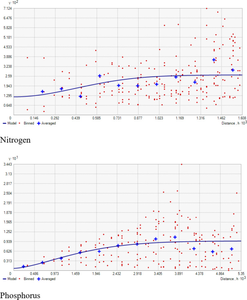
Fitted semi-variogram models for available soil macronutrients.

Fig. 5.

Fitted semi-variogram models for available soil micronutrients.

Fig. 6.

Effect of land use and management history on soil properties. The middle line of the box represents the median, and the lower and upper lines represent the lower and upper quartiles. Outliers are shown as points outside the box.

Fig. 7.

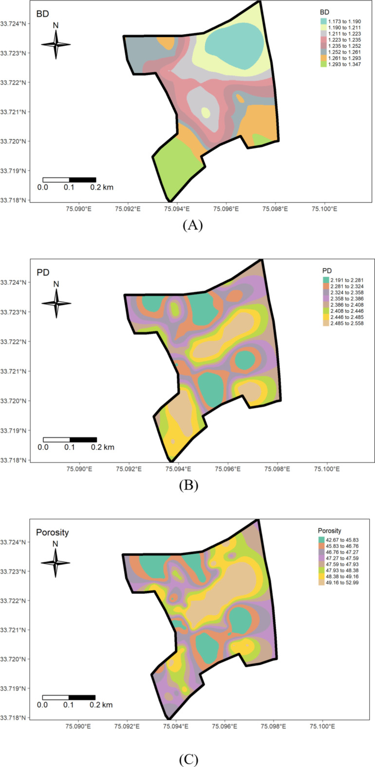
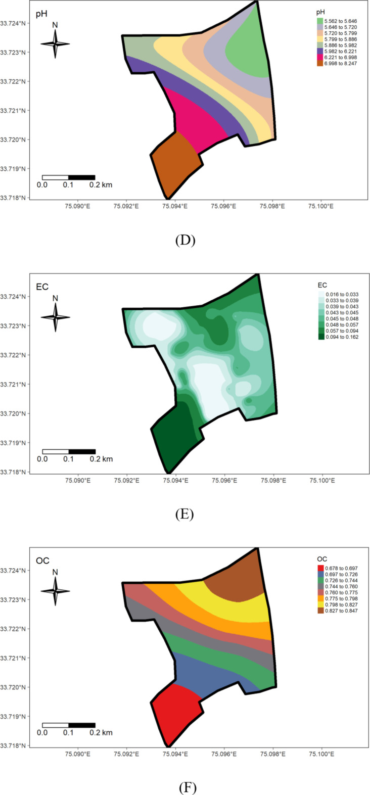
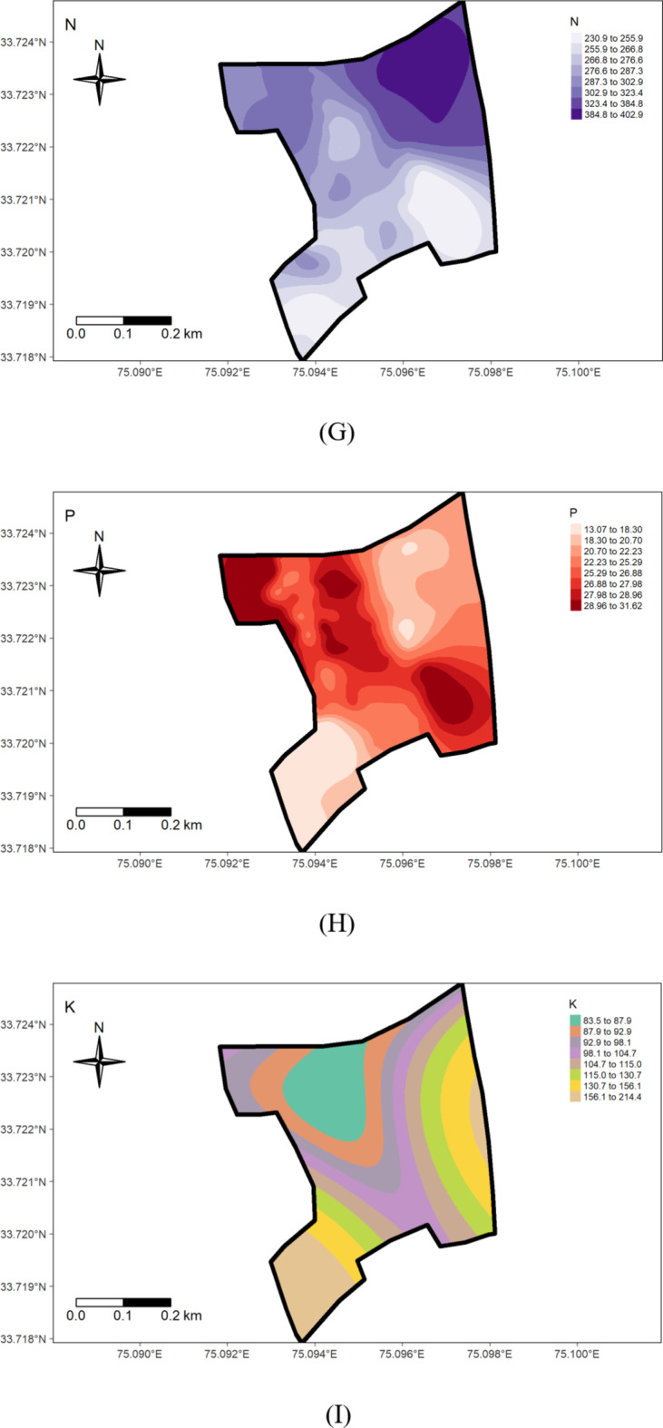
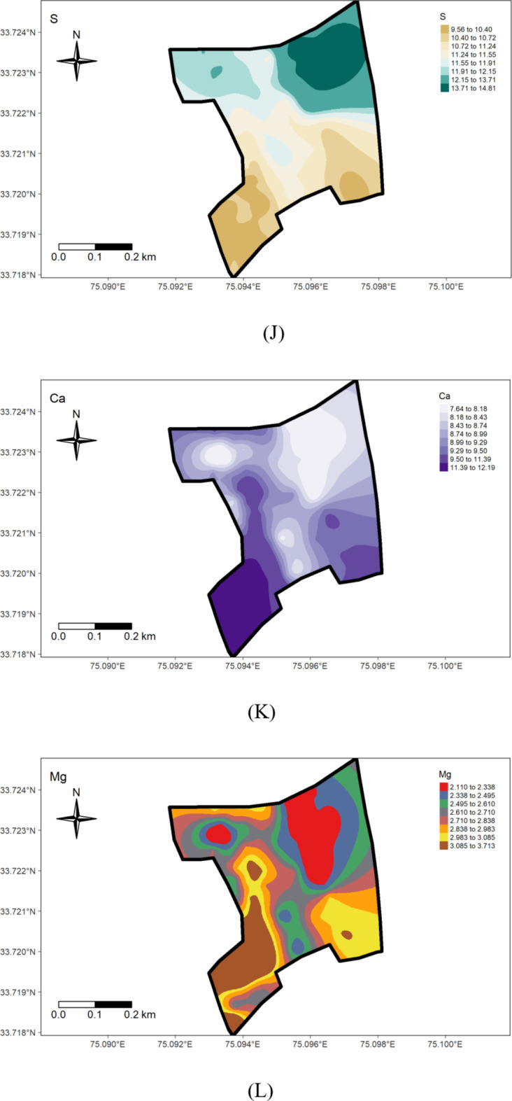
Spatial distribution maps of measured soil properties.

The improvement in the physical properties, especially in the northeast part of the rice-grown area, can be mainly ascribed to the beneficial impact of green manuring. This practice, consistently adopted during Rabi seasons over the past decade, has facilitated the incorporation of organic matter, resulting in concurrent increases in porosity and decreases in bulk density and particle density. The improvement in physical properties, particularly in the rice-grown area, suggests that expanding green manuring practices into other areas could help restore soil health, enhance water retention, and boost nutrient availability. Conversely, the higher bulk density values observed in the wheat-grown area (southwestern part) may be related to its comparatively lower organic matter content.

Chemical properties

Soil pH, the so-called “master variable, is a critical factor affecting microbial activity, nutrient availability & toxicity, and root growth, etc. The soils in the research farm displayed a pH range from strongly acidic (5.3) in the rice-grown area to slightly alkaline (8) in the wheat-grown area), with an average of 6.27. The coefficient of variation (CV) at 11.50% indicates medium variability, consistent with Yan et al.‘s (2019) findings, which reported a CV value of 17.18% for soil pH (Table 1) (Fig. 3). The lower pH in rice-grown areas may be attributed to prolonged use of ammoniacal (DAP) and ammonium-forming (urea) fertilizers³⁹ or the influence of high organic matter content, releasing organic acids during decomposition. Large evidence also indicates that excessive fertilizer application and removal of base cations through crop harvesting significantly contribute to soil acidification in agricultural systems⁴⁰. Similar findings were reported by Ramzan et al.⁴¹, which link pH decline in agricultural soils to lower basic cation saturation and/or organic acid production. The observed pH variation across the farm suggests that soil acidification in rice areas should be mitigated through appropriate management practices, while pH adjustment in wheat-growing areas could improve nutrient availability, especially for phosphorus. The wheat field’s highest pH value (8.0) (Fig. 7D) could be associated with land use practices and management history (Fig. 6D). Many studies have underscored the significant impact of land use on the spatial distribution of soil properties⁴¹.

Electric conductivity (EC) is an important indicator of soil health. Soils with EC values lower than 1 dS m^− 1 are ideal for plant growth. The EC values in the soils under study (Table 1; Fig. 7E) ranged from 0.01 d Sm^− 1 to 0.18 dS m^− 1, with mean values of 0.05 dS m^− 1 and variability coefficient of 62.89%. This agrees with Mansoor’s⁴² (2022) findings which recorded electrical conductivity in the range of 0.08 to 0.18 dS m^− 1 in Kashmir soils. Furthermore, considerable variation in EC corroborates with findings by Tekin et al.⁴⁴, who, in their study on soils in Turkey, reported EC exceeding 35% CV, indicating a strong degree of variability. The observed differences may be attributed to variations in soil management history, cropping system nutrient management, and irrigation practices (Fig. 6E). The high variability in EC suggests that localized management practices could influence soil salinity. Future farm practices should consider optimal irrigation and nutrient management to manage salt buildup, particularly in areas with higher EC.

The organic carbon content ranged from 0.52 to 1.21%, with a mean value of 0.75% (Table 1). This observation corroborates with Mahapatra et al.⁴⁵, who reported that organic carbon content ranges from 0.2 to 1.6% in certain soil profiles of the Kashmir valley. The coefficient of variation for soil organic carbon in the field was 20.89%, indicating a high degree of variability, possibly influenced by differences in land use type (Fig. 6F) & management history. The variability in organic carbon suggests that areas with lower organic matter, especially in wheat fields, could benefit from more intensive organic management practices such as green manuring or composting to improve soil fertility. The variability in organic matter content could also be attributed to intensive tillage practices in certain areas over the past few decades without sufficient external application of organic matter. Notably, areas with high organic matter correspond to locations where green manuring has been consistently practised for nearly a decade (Fig. 7F). The coefficient of variability was 20.89%. This observation is in agreement with the findings of Bangroo et al.⁴⁵, who reported a 30.0% coefficient of variation for organic carbon, indicating a high degree of variability in the soils of the Kashmir valley.

Geostatistical analyses, detailed in Table 2, showed that the Gaussian model best-suited pH, while EC and OC found their optimal fit in the Spherical model. Model selection was based on root mean squared error values. The nugget/sill ratio (C₀/(C₀ + C₁)) for pH, EC, and OC (0.01, 0, and 0.04%, respectively) suggested strong spatial dependence. Similar results are also indicated by Tesfahunegn et al³⁸. The range values were 9.33, 7.62, and 1.32 for pH, EC, and OC, respectively. This suggests that the sampling intensity employed in the present study may not have been adequately intensive to capture the spatial variability comprehensively. Notably, range values as low as 6 m for soil organic matter have been reported previously by Negassa et al.²⁰ in the Warnow Valley soils of Northern Germany.

Available macro-nutrients

The present study shows that nitrogen availability ranged from 187.80 to 455.83 kg ha^− 1, with a mean of 296.75 kg ha^− 1 (Table 1). The coefficient of variability was 19.69%, indicating a medium variation in the soils. The minimum available N (187.80 kg ha^− 1) was recorded in the wheat growing section (Fig. 6G) and can be attributed to the low organic matter content, nutrient management, crop demand, and previous cropping history (Fig. 7G). A positive correlation between organic carbon (OC) and soil nitrogen was observed (Table 3), aligning with the observations of Ye et al.⁴⁷. These results agree with the findings of Maqbool et al.³⁶, who recorded 175.1 to 485.1 kg ha^− 1 of available nitrogen in the agricultural soils of Kashmir valley. The nitrogen deficiency observed in wheat-growing areas suggests the need for nitrogen supplementation through targeted fertilization strategies to optimize crop yields.

Table 3.

Pearson correlation matrix showing the relationship among the studied soil properties.

	pH	OC (%)	AN (kg ha¯¹)	AP (kg ha¯¹)	AK (kg ha¯¹)	AS (mgkg¯¹)	AZn (mgkg¯¹)	AFe (mgkg¯¹)	AMn (mgkg¯¹)	ACu (mgkg¯¹)	Ex. Ca (cmolkg¯¹)	Ex. Mg (cmol kg¯¹)
pH	1.000
OC (%)	−0.558**	1.000
AN (kg ha¯¹)	−0.390**	0.823**	1.000
AP (kg ha¯¹)	−0.630**	−0.100NS	−0.126NS	1.000
AK (kg ha¯¹)	0.852**	−0.331**	−0.239*	−0.684**	1.000
AS (mgkg¯¹)	−0.594**	0.789**	0.704**	0.059NS	−0.430**	1.000
AZn(mgkg¯¹)	−0.665**	0.824**	0.641**	0.094NS	−0.413**	0.684**	1.000
AFe (mgkg¯¹)	−0.689**	0.091NS	0.047NS	0.749**	−0.705**	0.196NS	0.218*	1.000
AMn(mgkg¯¹)	−0.879**	0.303**	0.171NS	0.751**	−0.874**	0.396**	0.459**	0.854**	1.000
ACu(mgkg¯¹)	−0.635**	−0.028NS	−0.149NS	0.751**	−0.746**	0.146NS	0.123NS	0.760**	0.835**	1.000
Ex. Ca (cmol kg¯¹)	0.879**	−0.566**	−0.426**	−0.492**	0.829**	−0.644**	−0.676**	−0.628**	−0.822**	−0.601**	1.000
Ex. Mg (cmol kg¯¹)	0.598**	−0.509**	−0.354**	−0.217*	0.490**	−0.538**	−0.636**	−0.353**	−0.542**	−0.327**	0.813**	1.000

Pearson correlation analysis was conducted at a significance level of 0.05.

The symbols * and ** indicate significance at p ≤ 0.05, and p ≤ 0.01 respectively, while NS denotes a non-significant correlation.

The available phosphorus content in the research farm ranged from 12.04 to 33.07 kg ha^− 1, with a mean value of 23.61 kg ha^− 1 (Table 1). The coefficient of variability for phosphorous was 24.20%, suggesting high variation in the soils. The highest value (33.07 kg ha^− 1) was observed in the rice-grown area (Fig. 7H), possibly due to extensive applications of phosphatic fertilizers, especially DAP, to rice (Fig. 6H) and rapeseed crops over several decades, leading to phosphorus buildup in the soils. Conversely, the lowest value noted in the wheat-grown area could be due to insufficient application of phosphatic fertilizers, leading to phosphorus depletion. These findings underscore the need for site-specific treatments for effective and sustainable soil and crop management in the research farm. The observed phosphorus depletion in the wheat-growing area highlights the need for a more balanced fertilization approach, especially for phosphorus, to maintain soil fertility and optimize crop production.

The status of available potassium content in examined soil samples ranged from 77.57 to 195.87 kg/ha in the wheat-grown area (Fig. 7I), with an average value of 112.38 kg/ha (Table 1), (Fig. 6I). The coefficient of variability for potassium was 31.72%, indicating very high variation in the soil. The findings highlight an overall potassium-deficient status and huge within-field spatial variability in the examined soils, possibly attributed to variation in management practices and prolonged intensive cropping sequences with inadequate use of potassium fertilizers. This underscores the need for a reassessment and revision of potassium management practices on the research farm to address the area’s specific requirements and prevent further depletion of this critical element. Future nutrient management strategies should prioritize building up potassium levels above critical levels. Further, the results presented in Table 1 reveal that Sulphur (S) content in the research farm soils varied from 8.30 to 15.90 mg/kg, with a mean of 11.27 mg/kg. These results corroborate Maqbool’s³⁶ findings, showing 6.5 to 18.00 mg kg^− 1 sulphur in the Ganderbal district of Kashmir soils. The coefficient of variability for sulfur was 12.75%, suggesting medium variation in the soils. Throughout the research farm, sulfur levels were low, except in the portion subjected to green manuring for about the last decade, where sulfur content fell within the medium range. The lowest values were observed on the south-western side (Figs. 6 J & 7 J). The deficiency of sulfur in the examined soils may be attributed to the prolonged cultivation of rapeseed crops (brown sarson), leading to sulfur mining, a crucial component of the oil content. The medium levels of sulfur in the green manuring area are likely due to a relatively high level of soil organic matter. Sulfur deficiency may also result from using high-analysis-low-S-fertilizers, low sulfur returns with organic manure, and high-yielding varieties. Insufficient sulfur supply can impact crop yield and health, affecting protein and enzyme synthesis, chlorophyll synthesis, and seed oil content⁴⁸. Therefore, to achieve sustainable crop production, sulfur fertilizers should be applied to the area’s soils on a site-specific basis throughout the research farm.

The examination of data reveals that the Exchangeable Calcium in the research farm ranges from 7.10 to 12.40 cmol(+)kg^− 1, with a mean value of 9.48 cmol(+)kg^− 1 (Table 1; Fig. 4). Exchangeable Magnesium ranged from 1.80 to 3.90 cmol(+)kg^− 1, averaging 2.82 cmol(+)kg^− 1. These results are consistent with the findings of the literature reported by Maqbool³³—the coefficient of variation for ex. Ca and Mg were 15.11% and 18.75%, respectively, indicating a medium variation in the soil. The higher level of calcium content in the wheat-cultivated area (Fig. 7 K, J). suggests a significant influence on the management practices (Fig. 6 K, L).

Geostatistical analyses of soil macro-nutrients (Table 2) indicate that the Spherical model is a suitable fit for N, P, S, Exchangeable Ca, and Mg, while the Gaussian model fits for K (Fig. 3). The nugget/sill ratio (C₀/(C₀ + C1)) for P, K, and Ex. Ca stands at (0.07, 0.02, 0%), signifying strong spatial dependence. For N and S, ratios of (0.45 and 0.48%) suggest moderate spatial dependence, while Ex. Mg exhibits a weak spatial dependence with a ratio of (0.84). The nugget-to-sill (N: S) ratio in Table 2 indicates moderate spatial dependence for Nitrogen and Sulphur, strong for Phosphorus, Potassium, and Exchangeable Calcium, and weak for Exchangeable Magnesium. The near-zero slope observed in the case of Exchangeable Magnesium suggests a nearly random distribution pattern across the studied area. The corresponding range values for these nutrients were 1.07, 3.56, 0.84, 0.93, 1.32, and 2.88 for Nitrogen, Phosphorus, Potassium, Sulphur, Exchangeable Calcium, and Exchangeable Magnesium, respectively. The considerable spatial variability and small ‘range’ values observed in the field could result from diverse nutrient experimental trials that involved the application of various fertilizer treatments within small plots, typically spanning only a few meters. Stark et al.⁴⁹ reported range values as low as 0.13 m for certain soil parameters in the research farm of Lincoln University, New Zealand.

Available micronutrients

The availability of micronutrients under different land uses at the Research Farm revealed a range of 11.62 to 34.67 mg kg^− 1 for Iron, with a mean value of 22.56 mg kg^− 1, 12.8 to 35.80 mg kg^− 1 for Manganese, averaging 27.03 mg kg-1, 0.61 to 8.20 mg kg^− 1 for Copper, with a mean value of 3.50 mg kg^− 1, and 0.42 to 1.39 mg kg^− 1 for Zinc, with an average value of 0.74 mg kg^− 1 (Table 1; Fig. 5). These values are consistent with the literature reported by Wani et al.^50,] who recorded mean values for Fe, Mn, Cu, and Zn as 22.05, 18.59, 0.77, and 0.64 mg kg^− 1, respectively, in soils of J & K. The research farm soils were high in micronutrient status, except for zinc, which was deficient. The micronutrient sufficiency in the study area can be ascribed to the mainly acidic soil pH, as micronutrient availability increases with soil acidity. The relatively low micronutrient content in the wheat-grown area (Fig. 6 M, N,O, P) could be due to higher pH. The widespread zinc deficiency in the farm could be attributed to prolonged cultivation spanning over 8 decades of rice, a zinc-loving crop. Amanullah & Inamullah,^51,52 reported that the substantial increase in growth and yield of high-yielding rice genotypes caused considerable decreases in zinc concentration in soils. This suggests that an inadequate amount of zinc fertilizers is added to the soil to compensate for the loss of zinc in crop uptake and other losses. Therefore, to ensure sustainable soil health and crop production, a revised zinc management program must be tailored to suit the site-specific requirements of the research farm. This study uncovers a critical zinc deficiency linked to long-term rice cultivation, offering novel insights into micronutrient management for sustainable intensification in temperate rice-based systems.

The geostatistical analyses of (Fe, Mn, Cu, and Zn) as presented in Table 2, indicated that the suitable model for iron was Exponential, for Manganese was Gaussian, and the Spherical model best fitted Copper and Zinc. The nugget/sill ratio C₀/(C₀ + C1) for Fe, Mn, Cu, and Zn (0.13, 0.01, 0, 0.17%) suggested strong spatial dependence for micronutrients. Spatial distribution maps for Iron (Fe), Manganese (Mn), Copper (Cu), and Zinc (Zn) are depicted in Fig. 7M, N,O, P), respectively. The nugget-to-sill (N: S) ratio in Table 2 indicates a strong spatial dependence for all four studied micronutrients. The corresponding range values for these nutrients were 0.92, 10.26, 1.41, and 0.93, 1.23, and 2.88 for Iron (Fe), Copper (Cu), Manganese (Mn), and Zinc (Zn), respectively. The very small ‘range’ values observed in the field again underscore that the sampling intensity employed hasn’t been sufficient to capture the spatial variability comprehensively. The differential ranges of spatial dependence among the soil properties may be ascribed to variations in response to management practices, land use-cover, physical disturbances, etc. To address this challenge, it is recommended that future sampling strategies adopt shorter sampling distances to obtain more reliable results.

Correlations among the measured soil properties

The correlation analysis revealed significant relationships among the studied soil properties, reflecting their interdependence (Table 3). Soil pH exhibited strong negative correlations with organic carbon (OC: -0.558), available nitrogen (AN: -0.390), sulfur (AS: -0.594), zinc (AZn: -0.665), and micronutrients such as iron (AFe: -0.689), manganese (AMn: -0.879), and copper (ACu: -0.635). These relationships indicate that acidic conditions favor organic matter accumulation and enhance micronutrient availability, consistent with findings by Behera et al.¹. Organic carbon (OC) demonstrated strong positive correlations with AN (0.823) and AS (0.789), highlighting its critical role in nutrient retention and availability. OC also showed a significant positive correlation with zinc (AZn: 0.824), emphasizing the importance of organic matter in maintaining micronutrient availability. Exchangeable calcium (Ex. Ca) and magnesium (Ex. Mg) were positively correlated (0.813), reflecting their similar behavior in soil.

Phosphorus (AP) and potassium (AK) exhibited contrasting trends. AP was negatively correlated with pH (-0.630) and showed no significant relationship with OC (-0.100 NS). In contrast, AK showed a strong positive correlation with pH (0.852) and a negative correlation with OC (-0.331). The negative correlation between AP and AK (-0.684) further underscores the need for balanced fertilization to avoid antagonistic effects on nutrient availability.

Micronutrients such as iron (AFe), manganese (AMn), and copper (ACu) were strongly intercorrelated (AFe-AMn: 0.854; AFe-ACu: 0.760; AMn-ACu: 0.835), indicating their shared dependence on soil pH and organic matter. Zinc (AZn) showed moderate correlations with OC (0.824) and AS (0.684), but its overall deficiency in the study area highlights the need for targeted zinc fertilization, particularly in rice-grown zones where prolonged cultivation has depleted soil reserves.

Overall, the correlations underscore the complex interactions among soil properties and emphasize the importance of integrated, site-specific management strategies to address spatial variability, optimize nutrient availability, and promote sustainable agricultural practices.

Summary and conclusion

This study provides a comprehensive appraisal of farm-scale soil spatial variability at the MRCFC-Khudwani research farm, revealing significant heterogeneity in both physical and chemical soil properties. Geostatistical analysis demonstrated strong spatial dependence for bulk density, porosity, pH, EC, OC, P, K, Ex. Ca, Fe, Mn, Cu, and Zn; moderate dependence for particle density, N, and S; and weak dependence for Ex. Mg. Soil pH ranged from strongly acidic (5.3) in rice-grown areas to slightly alkaline (8.0) in wheat-grown areas, while organic carbon varied from 0.52 to 1.21%, reflecting high variability due to historical land use and fertilization practices. The spatial distribution of available nutrients showed high phosphorus buildup in rice-growing areas (up to 33.07 kg ha⁻¹) and severe potassium depletion in wheat-growing areas (as low as 77.57 kg ha⁻¹), highlighting the impact of long-term nutrient mismanagement. Zinc deficiency was widespread (0.27–1.64 mg kg⁻¹), particularly in continuously cultivated rice fields, underscoring the need for targeted micronutrient interventions. The findings emphasize the necessity of site-specific soil management strategies to optimize nutrient use efficiency and maintain soil health. The spatial distribution maps generated in this study provide a practical framework for precision nutrient management, optimized experimental site selection, and sustainable land-use planning at the research farm.

While this study offers valuable insights, certain limitations remain. The sampling intensity, although sufficient for broad-scale assessments, may not have fully captured micro-scale variability. Further, the study did not account for seasonal variations in soil properties, which could influence nutrient availability over time. Future research should focus on higher-resolution sampling grids to refine spatial predictions and incorporate remote sensing techniques for real-time soil monitoring. Moreover, integrating machine learning models with geostatistical techniques could enhance the accuracy of soil mapping and improve decision-making.

Author contributions

Conceptualization, R.K., A.H.L., and Z.A.S.; methodology, R.K., and A.H.L.; software, Z.A.S., and E.A.D., L.A.A., L.A.A., A.H. and B.S.; validation, M.A.G.,J.A.B. ; formal analysis, L.A.A., L.A.A., M.A.A., A.H, and S.S., L.A.A., L.A.A., A.H. and B.S. investigation, O.A.W.; resources I.A.J., and F.J.W.; data curation, L.A.A., L.A.A.; M.A.G.,J.A.B.; writing—original draft preparation Z.A.B.,N.R.S., and T.M.; writing—review and editing, L.A.A., L.A.A.; R.K., A.H., B.S., M.S., S.S. and Z.A.S.; visualization, R.K., and A.H.L.; supervision, M.S., S.S., M.A.G., and J.A.B .; project administration, I.A.J., and F.J.W. funding acquisition, L.A.A., L.A.A. and S.S., All authors have read and agreed to the published version of the manuscript.

Funding

The authors wish to thank Princess Nourah bint Abdulrahman University Researchers Supporting Project (number PNURSP2025R365), Princess Nourah bint Abdulrahman University, Riyadh, Saudi Arabia, for supporting this study.

Data availability

The datasets used and/or analysed during the current study available from the corresponding author on reasonable request.

Declarations

Competing interests

The authors declare no competing interests.

References

- 1.Behera, S. K. et al. Spatial variability of some soil properties varies in oil palm (Elaeis guineensis Jacq.) plantations of West coastal area of India. Solid Earth. 7, 979–993. 10.5194/se-7-979-2016 (2016). [Google Scholar]
- 2.Shukla, A. K. et al. Spatial variability of soil micronutrients in the intensively cultivated trans-genetic plains of India. Soil Tillage. Res.163, 282–289. 10.1016/j.still.2016.07.004 (2016). [Google Scholar]
- 3.Kathumno, V. M. Establishment of Soil Management Zones Based on Spatial Variability of Soil Properties for Precision Agriculture Using GIS in Katumani, Machakos District of Kenya. MSc. Thesis. University of Nairobi. (2007).
- 4.Bhatt, R. & Dwivedi, D. K. Digital soil mapping of PAU-Regional Research Station, Kapurthala, Punjab, India. Article Proc. Indian Natl. Sci. Acad. 88, 205–212 10.1007/s43538-022-00077-2 (2022).
- 5.Li, C., Wang, X. & Qin, M. Spatial variability of soil nutrients in seasonal rivers: A case study from the Guo river basin, China. Public. Libr. Sci. ONE. 16 (3), e0248655. 10.1371/journal.pone.0248655 (2021). [DOI] [PMC free article] [PubMed] [Google Scholar]
- 6.Brevik, E. C. et al. Soil mapping, classification, and pedologic modeling: history and future directions. Geoderma264, 256–274. 10.1016/j.geoderma.2015.05.017 (2015). [Google Scholar]
- 7.Pandey, S. et al. Improving fertilizer recommendations for Nepalese farmers with the help of soil-testing mobile Van. J. Crop Improv.32, 19–32. 10.1080/15427528.2017.1387837 (2018). [Google Scholar]
- 8.Aubert, B. A., Schroeder, A. & Grimaudo, J. IT as enabler of sustainable farming: an empirical analysis of farmers adoption decision of precision agriculture technology. Decis. Support Syst.54 (1), 510–520. 10.1016/j.dss.2012.07.002 (2012). [Google Scholar]
- 9.Eastwood, C., Klerkx, L. & Nettle, R. Dynamics and distribution of public and private research and extension roles for technological innovation and diffusion: case studies of the implementation and adaptation of precision farming technologies. J. Rural Stud.49, 1–12. 10.1016/j.jrurstud.2016.11.008 (2017). [Google Scholar]
- 10.Lindblom, J., Lundström, C., Ljung, M. & Jonsson, A. Promoting sustainable intensification in precision agriculture: review of decision support systems development and strategies. Precis. Agric.18 (3), 309–331. 10.1007/s11119-016-9491-4 (2017). [Google Scholar]
- 11.Kerry, R. & Oliver, M. A. Comparing sampling needs for variograms of soil properties computed by the method of moments and residual maximum likelihood. Geoderma140, 383–396. 10.1016/j.geoderma.2007.04.019 (2007). [Google Scholar]
- 12.Lagacherie, P. Digital soil mapping: a state of the art. In.: Hartemink AE, McBratney A, Mendonça-Santos M, de L, (Eds.). Digital Soil Mapping with Limited Data. 10.1007/978-1-4020-8592-5_1 (2008).
- 13.Saito, H., McKenna, A., Zimmerman, D. A. & Coburn, T. C. Geostatistical interpolation of object counts collected from multiple strip transects: ordinary kriging versus finite domain kriging. Stoch. Env Res. Risk Asst. 19, 71–85. 10.1007/s00477-004-0207-3 (2005). [Google Scholar]
- 14.Mandal, U. K., Sharma, K. L., Ghosh, P. K. & Mandal, B. Assessment of Spatial variability and mapping of soil properties for sustainable agricultural production using geographic information system techniques (GIS). Cogent. Food Agric.3 (1). 10.1080/23311932.2017.1279366 (2017).
- 15.Munyao, J. N., Macharia, P. N. & Mutua, B. M. Assessing Spatial variability of selected soil properties in upper Kabete campus coffee farm, university of Nairobi, Kenya. Int. J. Environ. Res. Public Health. 19 (16), 10045 https://pmc.ncbi.nlm.nih.gov/articles/PMC9424958/ (2022). [DOI] [PMC free article] [PubMed] [Google Scholar]
- 16.Gómez, D., White, J. G. & Whelan, B. M. Spatial variability in precision agriculture. In J. Stafford (Ed.), Precision Agriculture for Sustainability (pp. 1652–1674). Springer. https://link.springer.com/referenceworkentry/10.1007/978-3-319-17885-1_1652 (2020).
- 17.Amirinejad, A. A. et al. Assessment and mapping of Spatial variation of soil physical health in a farm. Geoderma160, 292–303. 10.1016/j.geoderma.2010.09.021 (2011). [Google Scholar]
- 18.Shukla, A. K. et al. Pre-monsoon Spatial distribution of available micronutrients and sulphur in surface soils and their management zones in Indian Indo-Gangetic plain. PLoS ONE. 15 (6), e0234053. 10.1371/journal.pone.0234053 (2020). [DOI] [PMC free article] [PubMed] [Google Scholar]
- 19.Wang, R., Zou, R., Liu, J., Liu, L. & Hu, Y. Spatial distribution of soil nutrients in farmland in a hilly region of the Pearl river delta in China based on geostatistics and the inverse distance weighting method. Agriculture11, 50. 10.3390/agriculture11010050 (2021). [Google Scholar]
- 20.Negassa, W., Baum, C., Schlichting, A., Müller, J. & Leinweber, P. Small-scale Spatial variability of soil chemical and biochemical properties in a re-wetted degraded peatland. Front. Environ. Sci.7, 116. 10.3389/fenvs.2019.00116 (2019). [Google Scholar]
- 21.Gupta, R. P. & Dakshinamoorthy, C. Procedures for Physical Analysis of Soils and Collection of Agrometeorological Data, Division of Agricultural Physics (Indian Agricultural Research Institute, 1980).
- 22.Jalota, S. K., Khera, R. & Ghuman, B. S. Methods in Soil Physics, Narosa Publishing House, New Delhi. 65–67 (1998).
- 23.Rattan, R. K. Fundamentals of soil science. National Agricultural Sci. Centre Complex. New. Delhi91 (2009).
- 24.Jackson, M. L. Soil Chemical Analysis (Prentice Hall of India Private Limited, 1973).
- 25.Walkley, A. J. & Black, C. A. An Estimation of the Degtjareff method for determining soil organic matter and a proposed modification of the chromic acid Titration method. Soil Sci.37, 29–38. 10.1097/00010694-193401000-00003 (1934). [Google Scholar]
- 26.Subbiah, B. V. & Asija, G. L. A rapid procedure for the Estimation of available nitrogen in soils. Curr. Sci.25, 259–260 (1956). [Google Scholar]
- 27.Olsen, S. R., Cole, C. V. & Watanabe, F. S. and Dean. L. A. Estimation of available phosphorus in soils by extraction with sodium carbonate. U S Department Agric. Circular 939 (1954).
- 28.Richard, L. A. Diagnosis and improvement of saline and alkali soils. USDA. Hand Book No. 80. Oxford and IBH Publishing Co. Kolkata, Bombay, New Delhi. (1954).
- 29.Chesnin, L. & Yien, C. H. Turbidimetric determination of available sulphur. Proc. Soil Sci. Soc. Am. 15, 149–151 (1951).
- 30.Lindsay, W. L. & Norvell, W. A. Development of a DTPA soil test for zinc, iron, manganese and copper. Soil Sci. Soc. Am. J.42, 421–428 (1978). [Google Scholar]
- 31.Triantafilis, J., Odeh, I. & McBratney, A. Five Geostatistical models to predict soil salinity from electromagnetic induction data across irrigated cotton. Soil Sci. Soc. Am. J.65, 869–878. 10.2136/sssaj2001.653869x (2001). [Google Scholar]
- 32.Li, C., Wang, X. & Qin, M. Spatial variability of soil nutrients in seasonal rivers: A case study from the Guo river basin, China. Public Libr. Sci.. 16 (3), e0248655. 10.1371/journal.pone.0248655 (2021). [DOI] [PMC free article] [PubMed] [Google Scholar]
- 33.Cambardella, C. A. & Karlen, D. L. Spatial analysis of soil fertility parameters. Precis. Agric.1, 5–14. 10.1023/A:1009925919134 (1999). [Google Scholar]
- 34.USDA (United States Department of Agriculture) Staff. Soil Quality Kit Guide (USDA-NRCS-ARS-SQI, 1999).
- 35.Abad, J. R. S., Khosravi, H. & Alamdarlou, E. S. Assessment of the effects of land use changes on soil physicochemical properties in Jafarabad Golestan Province, Iran. Bull. Environ. Pharmacol. Life Sci.3 (3), 296–300 (2014). [Google Scholar]
- 36.Rasool., M. M. & Ramzan, S. R. Soil physico-chemical properties as impacted by different land use systems in district Ganderbal, Jammu and Kashmir: India. Int. J. Chem. Stud. 5(4), 832–840. (2007)
- 37.Haque, A. A. M., Jayasuriya, H. P. W., Salokhe, V. M., Tripathi, N. K. & Parkpian, P. Assessment of Influence and Inter-Relationships of Soil Properties in Irrigated Rice Fields of Bangladesh by GIS and Factor Analysis. Agric. Eng. Int. CIGR E-J. (2017).
- 38.Tesfahunegn, G. B., Tamene, L. & Vlek, P. L. G. Catchment-scale Spatial variability of soil properties and implications on site-specific soil management in Northern Ethiopia. Soil. Tillage Res.117, 124–139. 10.1016/j.still.2011.09.005 (2011). [Google Scholar]
- 39.Haile, G., Lemenhi, M., Itanna, F. & Senbeta, F. Impacts of land uses changes on soil fertility, carbon and nitrogen stock under smallholder farmers in central highlands of Ethiopia: implication for sustainable agricultural landscape management around Butajira area. New. York Sci. J.7, 27–44 (2014). [Google Scholar]
- 40.Guo, X. et al. Drivers of spatio-temporal changes in paddy soil pH in Jiangxi Province, China from 1980 to 2010. Sci. Rep.8, 1–11 (2018). https://www.nature.com/articles/s41598-018-20873-5 [DOI] [PMC free article] [PubMed] [Google Scholar]
- 41.Ramzan, S., Bhat, M. A., Kirmani, N. A. & Rasool, R. Fractionation of zinc and their association with soil properties in soils of Kashmir Himalayas. Int. Invent. J. Agric. Soil Sci.2 (8), 132–142 (2018). [Google Scholar]
- 42.Fang-fang, S. et al. Spatial variability of soil properties in red soil and its implications for site-specific fertilizer management. J. Integr. Agric.19 (9), 2313–2325. 10.1016/S2095-3119(20)63221-X (2020). [Google Scholar]
- 43.Mansoor, M. et al. Effect of depth-wise distribution of physico-chemical properties of different land-use systems of district Baramulla of Kashmir. Pharm. Innov. J.11 (2), 2516–2519 (2022). [Google Scholar]
- 44.Tekin, A. B., Gunal, H., Sındır, K. & Balc, Y. Spatial structure of available micronutrient contents and their relationships with other soil characteristics and corn yield. Fresenius Environ. Bull.20, 775–783 (2011). [Google Scholar]
- 45.Mahapatra, S. K., Walia, C. S., Sidhu, G. S., Rana, K. P. C. & Tarsem, L. Characterization and classification of the soils of different physiographic unit in the subhumid ecosystem of Kashmir region. J. Indian Soc. Soil. Sci.48, 572–577 (2000). [Google Scholar]
- 46.Bangroo, S. A. et al. Quantifying Spatial variability of soil properties in Apple orchards of Kashmir, India, using Geospatial techniques. Arab. J. Geosci.14, 1–10. 10.1007/s12517-021-08457-6 (2021). [Google Scholar]
- 47.Ye, Y. et al. Predicting Spatial distribution of soil organic carbon and total nitrogen in a typical human impacted area. Geocarto Int. 1–19 (2021).
- 48.Jamal, A., Fazli, I. S., Ahmad, S., Abdin, M. Z. & Yun, S. J. Effect of sulphur and nitrogen application on growth characteristics, seed and oil yield of soybean cultivars. Korean J. Crop Sci.50, 340–345 (2005). [Google Scholar]
- 49.Stark, C. H. E., Condron, L. M., Stewart, A., Di, H. J. & O’Callaghanc, M. Small-scale Spatial variability of selected soil biological properties. Soil Biol. Biochem.36, 601–608. 10.1016/j.soilbio.2003.12.005 (2004). [Google Scholar]
- 50.Sharma, W. O. A. et al. Digital mapping of soil physicochemical properties of Ramban district of Jammu and Kashmir using geographic information system. Indian J. Ecol.49 (5), 1654–1660 (2023). [Google Scholar]
- 51.Amanullah & Inamullah Preceding rice genotypes, residual phosphorus and zinc influence harvest index and biomass yield of subsequent wheat crop under rice-wheat system. Pak J. Bot.47, 265–273 (2015). [Google Scholar]
- 52.Amanullah & Inamullah. Residual phosphorus and zinc influence wheat productivity under rice–wheat cropping system. Springer Plus. 5, 255. 10.1186/s40064-016-1907-0 (2016). [DOI] [PMC free article] [PubMed] [Google Scholar]
Associated Data
This section collects any data citations, data availability statements, or supplementary materials included in this article.
Data Availability Statement