Easy‐to‐use R functions to separate reduced‐representation genomic datasets into sex‐linked and autosomal loci, and conduct sex assignment

Abstract

Identifying sex‐linked markers in genomic datasets is important because their presence in supposedly neutral autosomal datasets can result in incorrect estimates of genetic diversity, population structure and parentage. However, detecting sex‐linked loci can be challenging, and available scripts neglect some categories of sex‐linked variation. Here, we present new R functions to (1) identify and separate sex‐linked loci in ZW and XY sex determination systems and (2) infer the genetic sex of individuals based on these loci. We tested these functions on genomic data for two bird and one mammal species and compared the biological inferences made before and after removing sex‐linked loci using our function. We found that our function identified autosomal loci with ≥98.8% accuracy and sex‐linked loci with an average accuracy of 87.8%. We showed that standard filters, such as low read depth and call rate, failed to remove up to 54.7% of sex‐linked loci. This led to (i) overestimation of population F _IS by up to 24%, and the number of private alleles by up to 8%; (ii) wrongly inferring significant sex differences in heterozygosity; (iii) obscuring genetic population structure and (iv) inferring ~11% fewer correct parentages. We discuss how failure to remove sex‐linked markers can lead to incorrect biological inferences (e.g. sex‐biased dispersal and cryptic population structure) and misleading management recommendations. For reduced‐representation datasets with at least 15 known‐sex individuals of each sex, our functions offer convenient resources to remove sex‐linked loci and to sex the remaining individuals (freely available at https://github.com/drobledoruiz/conservation_genomics).

1. INTRODUCTION

Population genetic datasets are a rich source of information for wildlife managers (Hoffmann et al., 2015; Hohenlohe et al., 2021). They provide data on genetic structure, adaptation and evolutionary trajectories of species and populations (e.g. local adaptation, hybridisation, population dynamics and evolutionary potential; Willi et al., 2022). They can reveal biological and ecological processes that could not otherwise be studied (e.g. mating systems and sex‐specific dispersal and gene flow; Amos et al., 2014; Ellegren, 2014). In addition, they help to identify genetic problems in small populations—notably loss of genetic diversity, inbreeding and inbreeding depression—and develop simple and cost‐effective management solutions towards their conservation (e.g. genetic augmentation, genetic rescue; Frankham et al., 2017; Harrisson et al., 2019; Kardos, 2021).

With the massive amount of genomic data that can be generated, the level of expertise in bioinformatics required for analysing genomic datasets has increased (Hohenlohe et al., 2021; Holderegger et al., 2019; McMahon et al., 2014). Conservation geneticists spend a great part of their time learning the use of new software, which reduces their availability to engage in other important activities needed to bridge the gap between research and conservation practice (e.g. facilitating communication with wildlife managers, building relationships with primary industry, informing and shaping policy; Britt et al., 2018; Galla et al., 2016; Taylor et al., 2017). Accordingly, there is much interest in creating easy‐to‐use resources to automate and streamline dataset filtering and genomic analyses. This has included the development of packages for R, which tends to be a more welcoming environment for biologists than does command‐line software (e.g. dartR: Gruber et al., 2018, Mijangos et al., 2022; SambaR: de Jong et al., 2021; snpR: Hemstrom & Jones, 2023; SNPfiltR: DeRaad, 2022, Hogg et al., 2022).

Most population genetic analyses assume autosomal loci; thus, best‐practice filtering includes the removal of sex‐linked loci from SNP datasets. If sex‐linked loci are not removed, estimates of population genetic diversity such as heterozygosity, Wright's fixation indices including F _IS, polymorphism, and allelic richness may be biased depending on the sex ratio of the sample and the sex‐chromosome‐to‐autosome diversity ratio (Allendorf et al., 2022; Ellegren, 2009; Frankham et al., 2017). Assessment of population genetic structure also benefits from the removal of sex‐linked loci because they can mask genetic structure that is due to evolutionary processes (e.g. gene flow, natural selection and genetic drift; Benestan et al., 2017; Pritchard et al., 2000; Radosavljević et al., 2015). Similarly, parentage analyses assume autosomal Mendelian inheritance, and so their accuracy can be affected by the presence of sex‐linked loci because they create apparent genetic mismatches between true parent‐offspring pairs (Jones & Wang, 2010). On the other hand, focusing on sex‐linked markers can help assign sex to individuals of sexually monomorphic species, as well as reveal interesting patterns of sex‐specific ecology and evolution (e.g. natural selection, philopatry; Arnold & Wilkinson, 2015; Castella et al., 2001; Pavlova et al., 2013). Thus, correct identification of sex‐linked loci is important for making appropriate management recommendations.

In animal species, the two most common chromosomal sex‐determination systems are XY and ZW. In an XY system, typical for mammals and some insects, males are the heterogametic sex with one X and one Y chromosome, and females are the homogametic sex with two X chromosomes. In contrast, in the ZW system, typical for birds and some reptiles and insects, females are heterogametic (ZW) and males are homogametic (ZZ) (Beukeboom & Perrin, 2014). The SNP markers on sex chromosomes can be classified into three types with different inheritance and characteristics (Figure 1; Käfer et al., 2021; Peneder et al., 2017):

1. Those present only on the W or Y chromosome (hereafter ‘W‐linked/Y‐linked’; Figure 1 in yellow). In SNP datasets, such markers are called only in the heterogametic sex and are missing in the homogametic sex.

2. Those present only on the Z or X chromosome (hereafter ‘Z‐linked/X‐linked’; Figure 1 in orange). In SNP datasets, the heterogametic sex possesses only one allele (i.e. they are hemizygous), and individuals appear homozygous when genotyped. The homogametic sex, which possesses two alleles, can be heterozygous or homozygous, as for an autosomal locus.

3. Those present in homologous regions of both sex chromosomes, Z and W or X and Y, and are similar enough to be considered alleles of the same locus (hereafter ‘gametologs’, Figure 1 in green). In some cases, gametologous loci have one allele that is found exclusively on one sex chromosome while the other allele appears exclusively on the other. As a result, all members of the heterogametic sex appear heterozygous, and the homogametic sex homozygous. These loci are known as ‘fixed’ gametologs and are common in old sex chromosomes. In other cases (e.g. in recently evolved [neo‐] sex chromosomes), the ‘Z‐allele’ (or ‘X‐allele’) is still found on some versions of the W (or Y) chromosome, and thus, some individuals of the heterogametic sex are homozygous. In these cases, the gametologs are ‘non‐fixed’.

FIGURE 1.

Schematic of the distribution patterns of three types of sex‐linked loci in the ZW sex‐determination system: W‐linked loci are found only in the W chromosome (yellow); Z‐linked loci are found only in the Z chromosome (orange); gametologous loci are present in both chromosomes (green). The same principles apply to the XY sex‐determination system, but males are heterogametic (XY) and females homogametic (XX).

The simplest way to distinguish sex‐linked loci from autosomal ones is to identify those found in reads that mapped to the sex chromosomes of the reference genome. However, this is not possible when (i) a reference genome is not available–as is the case for most wildlife species—and de novo genotyping is required, (ii) there is little conserved synteny between the studied genome and the reference, or (iii) the W/Y chromosome of the reference genome is fragmented into numerous unmapped scaffolds, as is common in many genome projects (Carvalho & Clark, 2013).

Some methods to identify sex‐linked SNPs have been developed. MendelChecker, for example, uses the deviation from Mendelian inheritance to calculate the probability that a specific SNP is sex‐linked, with the disadvantage that it requires genotype probabilities and pedigree information for analysis (Chen et al., 2014). Other methods use a set of individuals of known sex to test whether the allele frequencies of a given locus differ between the sexes. For instance, RADSEX is a command‐line software that uses identical raw reads as non‐polymorphic markers and uses their presence or absence in males and females to identify those significantly associated with sex (Feron et al., 2021). SDpop and the R method SATC require the mapping of raw reads to a reference genome in order to identify sex‐linkage (Käfer et al., 2021; Nursyifa et al., 2022). Some other studies have identified sex‐linked markers by testing for differentiation between the sexes using F _ST, but this approach can be used only for Z‐linked/X‐linked and gametologous loci (Benestan et al., 2017; Drinan et al., 2018; Trenkel et al., 2020). Function gl.report.sexlinked from dartR package (v2; Mijangos et al., 2022) uses arbitrary heterozygosity thresholds as default parameters to identify fixed gametologs and can be used to identify non‐fixed gametologs and Z‐linked/X‐linked loci by fine‐tuning parameters (Pavlova et al., 2022). Nevertheless, this approach has the disadvantages that there are no clear instructions on how to tune parameters, the user has to manually adjust thresholds on a trial‐and‐error basis for each genomic dataset, and its precision declines with low heterozygosity, risking either the erroneous removal of autosomal loci with rare alleles or the failure to remove sex‐linked loci with low heterozygosity. Overall, these methods could be improved upon by developing an intuitive statistical approach that systematically identifies and distinguishes among types of SNPs (autosomal, W‐linked/Y‐linked, Z‐linked/X‐linked, and gametologs) that is automated in a ready‐to‐use R function with little user intervention needed.

In the same way that it is possible to use a set of known‐sex individuals to identify sex‐linked loci, the opposite is also possible: use a set of known sex‐linked loci to identify the sex of an individual. Sex assignment is usually done utilising a handful of sex‐linked loci of only one type (Trenkel et al., 2020). For example, if using non‐fixed ZW‐gametologs (for which heterozygous individuals are never male), an individual is declared female if it is heterozygous for at least one locus, yet by chance, depending on allelic frequencies and the number of evaluated gametologs, some females may not be heterozygous for any of the loci. On the other hand, depending on genotyping error rates, some males may appear heterozygous for some loci. To our knowledge, despite the rich information that the three types of sex‐linked loci contain to improve sex assignment, the comparison of their information is rarely, if ever, done. Thus, the sexing of individuals using large SNP datasets can benefit from a methodical procedure that uses the information from all available sex‐linked loci and can be integrated as a standard step in bioinformatics pipelines.

Another best‐practice during filtering of autosomal and sex‐linked datasets is minimising the presence of ‘multilocus’ SNPs (also known as multilocus contigs, multicopy loci or homeologs; Hohenlohe et al., 2011; O'Leary et al., 2018; Willis et al., 2017). These artefactual SNPs arise during bioinformatic processing of raw reads and are the product of erroneously fusing multiple physically separate loci that are very similar because they are paralogs, repetitive elements or otherwise very much alike. Because a multilocus SNP is actually multiple loci, multilocus SNPs tend to present abnormally high read depths. This characteristic allows their removal by setting a maximum read depth threshold during filtering (usually twice the mode or mean; Willis et al., 2017). In some cases, there are fixed or near‐fixed differences between the artificially fused loci, which makes multilocus SNPs exhibit heterozygosity well‐above the expectation of 0.5 for biallelic markers at Hardy–Weinberg proportions. As a consequence, these SNPs can inflate estimates of heterozygosity (O'Leary et al., 2018). A common practice to identify these artefactual loci using heterozygosity is to set an arbitrary maximum threshold (e.g. heterozygosity ≥0.6). It has been found that using more than one approach to identify multilocus SNPs–and removing those that are flagged by any method—constitutes the best strategy (Willis et al., 2017).

Lastly, parentage analyses and sibship reconstruction using molecular markers have great relevance in wildlife conservation. Resolving unknown parent‐offspring relationships gives insights into the behaviour, ecology and evolution of plant and animal populations (e.g. extra‐pair mating, inbreeding avoidance, dispersal, natural selection and effective population size; Flanagan & Jones, 2019). Their application extends into very practical instances such as monitoring the success of translocations and genetic rescue, and spotting illegal trade of wild individuals (Fitzpatrick et al., 2020; Mucci et al., 2020; Van Rossum, 2022). Moreover, captive breeding programmes also benefit from parentage analyses that allow them to estimate founder relationships (typically assumed unrelated), validate pedigrees and correct errors (Galla et al., 2022; Moran et al., 2021; Overbeek et al., 2020). Among the variety of parentage analysis software in existence, one of the most popular is COLONY, which simultaneously infers sibship and parentage and can handle thousands of SNPs (Jones & Wang, 2010). However, handling large amounts of genetic data in order to format it into the specific input file for COLONY requires some degree of bioinformatics expertise (Flanagan & Jones, 2019). Often, researchers need to create different input files because several runs are usually required to maximise the detection of true relationships. This can be a time‐consuming task worth automating.

In this study, we aim to create four R functions to assist researchers analysing reduced‐representation genomic datasets. The study consists of three parts. First, we describe four R functions that we designed to automate common tasks in conservation genomic studies: (1) identify and remove sex‐linked loci (function filter.sex.linked), (2) use sex‐linked loci to identify the genetic sex of individuals (function infer.sex), (3) filter out excessively heterozygous loci that are likely to be genotyping errors (function filter.excess.het), and (4) create input files for parentage analyses in COLONY (function gl2colony). Second, we apply the functions on empirical genomic data for two bird and one mammal species with chromosome‐length reference genomes available and test the accuracy of functions filter.sex.linked and infer.sex. Third, we show how incomplete removal of sex‐linked loci affects downstream analyses of (i) population genetic diversity, (ii) individual heterozygosity, (iii) population genetic structure and (iv) parentage.

2. METHODS

2.1. Design of functions

The following four R functions were designed for SNP datasets, such as those produced by reduced‐representation technologies (DArT, RAD or ddRAD; Baird et al., 2008; Davey & Blaxter, 2010; Kilian et al., 2012; Peterson et al., 2012). The functions require the data to be imported to R as a genlight object (adegenet; Jombart & Ahmed, 2011). The functions make use of the information stored in genlight object's ‘ind.metrics’ (stored in slot ‘@other$ind.metrics’) as implemented by dartR package (Gruber et al., 2018; Mijangos et al., 2022). The functions and three small test datasets are available at https://github.com/drobledoruiz/conservation_genomics.

2.1.1. Function filter.sex.linked

Purpose

Detecting and filtering out sex‐linked loci.

Input

One genlight object with at least 30 individuals of known sex (15 of each sex; see Section 3), and a user‐specified parameter declaring the sex‐determination system of the species (‘zw’ or ‘xy’). Known sex is provided in ‘ind.metrics’ with a column named ‘sex’ and individuals assigned ‘F’ (females) or ‘M’ (males). Individuals with unknown sex (i.e. assigned anything other than ‘F’ or ‘M’) are ignored by the function.

How it works

The rationale behind this function is that the scoring rate and heterozygosity of autosomal loci should not differ between the sexes, but they do differ for sex‐linked loci. Based on this, the function works in two phases:

• Phase I. Use locus call rate to identify W‐linked/Y‐linked loci and other loci with sex‐biased call rates. The function counts, for each locus, the number of known females and the number of known males with NA (i.e. missing data) and with a called genotype (i.e. ‘0’, ‘1’ or ‘2’). These four counts are used to build a 2 × 2 contingency table per locus on which a Fisher's exact test is performed in order to test for the independence of call rate and sex (α = 0.01). The logic is that autosomal loci should present roughly the same call rate for males and females (Figure 2a, diagonal cloud in grey), and therefore, a locus in which one sex has significantly more missing data than the other is likely to be sex‐linked. The p‐values of all loci are adjusted for False Discovery Rate with R function p.adjust (Benjamini & Hochberg, 1995). Of the loci with adjusted p < 0.01, those whose male call rate is ≤ 0.1 are assigned as W‐linked (because males lack a W chromosome; Figure 2a, in yellow) or as Y‐linked if female call rate is ≤ 0.1 (because females lack a Y chromosome). The remaining loci with adjusted p < 0.01 are identified as ‘sex‐biased’ (Figure 2a, in blue).

• Phase II. Use locus heterozygosity to identify Z‐linked/X‐linked loci and gametologs. The function counts, for each locus, the number of known females and the number of known males that are heterozygous (i.e. ‘1’), and homozygous (i.e. ‘0’ or ‘2’). In the same way as for Phase I, these four counts are used to build a 2 × 2 contingency table per locus and to perform a Fisher's exact test to test for the independence of heterozygosity and sex (α = 0.01). Under the logic that autosomal loci should present no difference in the proportion of heterozygous individuals between sexes (Figure 2b, diagonal cloud in dark grey), a locus in which one sex has significantly more heterozygous individuals than the other is likely to be sex‐linked. p‐values are adjusted for False Discovery Rate with R function p.adjust (Benjamini & Hochberg, 1995). Of the loci with adjusted p < 0.01, those whose proportion of heterozygous males is greater than the proportion of heterozygous females are identified as Z‐linked (because females have only one Z chromosome and should be mainly scored as homozygous; Figure 2b, in orange). On the other hand, loci whose proportion of heterozygous females is larger than the proportion of heterozygous males are identified as gametologs (because males have two Z chromosomes, and thus should present only the Z‐associated allele and be scored as homozygous; Figure 2b, in green). The same logic, with reversed expectations for sexes, is applied to the XY sex‐determination system (X‐linked: proportion of heterozygous females > proportion of heterozygous males; gametologs: proportion of heterozygous males > proportion of heterozygous females).

The loci that are not identified as belonging to any category of sex‐linkage are inferred autosomal. The function finishes by splitting each category of loci into its own genlight object.

FIGURE 2.

Graphical representation of the expected call rate and proportion of heterozygous individuals for autosomal and sex‐linked loci. (a) Autosomal loci (grey) are expected to present roughly the same call rate for males and females. W‐linked loci (yellow) are expected to be called in females but absent in males because males lack a W chromosome. We refer to other loci whose call rate is biased by sex as ‘sex‐biased’ (blue, drawn here for male‐bias in call rate). (b) Autosomal loci (grey) are expected to present roughly the same proportion of heterozygous males and females. For Z‐linked loci (orange), females are expected to be homozygous because they have only one Z chromosome. For gametologous loci (green), males are expected to be homozygous because they have two Z chromosomes, each with the same Z‐associated allele.

Output

1. A list containing six elements: one table—with per‐locus counts, Fisher's exact test estimates, p‐values and true/false columns for each type of sex‐linked loci—and five genlight objects: one with autosomal loci, and one with each type of sex‐linked loci (Fig. 2).

2. Two sets of ‘before’ and ‘after’ plots: one set with female call rate plotted against male call rate with each data point representing one locus (one plot before and one plot after removing W‐linked/Y‐linked and sex‐biased loci identified by call rate). The other set with the proportion of heterozygous females plotted against the proportion of heterozygous males, each point representing one locus (one plot before and one after removing Z‐linked/X‐linked and gametologous loci identified by heterozygosity).

Recommended use

In order to minimise the number of loci analysed by the function to speed computation time, it is advantageous to use the filter.sex.linked function after the removal of secondary loci (i.e. those in the same sequenced fragment). This may not be needed when computation time is not a concern or the number of loci is smaller than 50,000 SNPs, which will help identify sex‐linked markers in species with short or little‐differentiated sex chromosomes. We also included the option of running the function in parallel, which reduces run time. Additionally, it is strongly recommended to use this function before other quality filters in order to ensure that (i) variation in call rate has not been truncated and (ii) downstream filtering is done on autosomal loci only. When known‐sex individuals are scarce, we recommend using at least 15 known‐sex individuals of each sex to identify as many sex‐linked loci as possible (even if few), then use those sex‐linked loci to sex all individuals with function infer.sex, and then use the new sex assignments to identify the remaining sex‐linked loci with function filter.sex.linked (see Sections 2.2.4 and 3.3).

2.1.2. Function infer.sex

Purpose

Identify the genetic sex of individuals.

Input

The output of function filter.sex.linked (list of six elements), a user‐specified parameter that declares the sex‐determination system of the species (‘zw’ or ‘xy’), and a seed number.

How it works

This function uses the types of loci available in the input (W‐linked/Y‐linked, Z‐linked/X‐linked and gametologous loci) to assign one preliminary sex for each type of sex‐linked loci:

• W‐linked/Y‐linked loci. For a ZW system, it preliminarily assigns ‘M’ (male) to an individual if it presents more loci with NA (i.e. missing data) than loci with called genotype (i.e. ‘0’, ‘1’ or ‘2’), and ‘F’ (female) otherwise. For an XY system, the assignment is the opposite.

• Z‐linked/X‐linked loci. It uses the matrix of genotypes for all individuals to perform k‐means clustering with two centres (using the provided seed number). The rationale is that individuals would form two distinctive clusters, one per sex. As a result, individuals are assigned to one of two sex clusters. The individual with the most loci scored as heterozygous is used to identify the sex of its cluster (‘M’ for ZW system and ‘F’ for XY system), while the other cluster is identified as the opposite sex.

• Gametologs. It identifies the five gametologous loci with the smallest adjusted p‐value (i.e. those that deviate the most from autosomal expectations) and performs k‐means clustering in which individuals are assigned to one of two sex clusters. It also uses the individual with the most loci scored as heterozygous to identify the sex of its cluster (‘F’ for ZW system, and ‘M’ for XY system).

If a type of sex‐linked locus was not available (e.g. less than five gametologs), it assigns NA to that preliminary assignment. The function uses the preliminary assignments to output a final sex assignment: ‘F’ or ‘M’ if all available preliminary assignments match, ‘*F’ or ‘*M’ if they do not.

Output

A table with the three preliminary and final sex assignments per individual. The table also includes the raw data on which the preliminary assignments were based on: the number of W‐linked/Y‐linked loci with missing/called genotype, the number of Z‐linked/X‐linked loci scored as homozygous/heterozygous and the number of gametologs scored as homozygous/heterozygous (even if < 5).

Recommended use

We created this function with the explicit intent that a person inspects the final sex assignments for which not all three preliminary assignments agree (denoted as ‘*M’ or ‘*F’). Some individuals may have ambiguous genotypes for one type of sex‐linked loci, and given the nature of k‐means clustering, they may be assigned the wrong preliminary sex. It is recommended that the user checks the output table to make a decision on the final assignment. We recommend this function being used straight after using function filter.sex.linked.

2.1.3. Function filter.excess.het

Purpose

Remove loci with excessively high heterozygosity that are suspected to be bioinformatic artefacts (i.e. multilocus SNPs).

Input

A genlight object in which ‘ind.metrics’ contains a column named ‘pop’, and each individual is assigned to one population.

How it works

This function considers a locus to be ‘excessively heterozygous’ if its heterozygosity exceeds 0.5 and it significantly deviates from Hardy–Weinberg (HW) proportions. The rationale is that applying an absolute heterozygosity cut‐off (e.g. 0.5 or 0.6) may remove some loci that conform to HW proportions but exceed the threshold due to sampling error (i.e. imperfect sampling of individuals or genotyping). The function starts by dividing the genlight object by population and identifying loci whose heterozygosity > 0.5. It then performs a χ ² test to detect significant heterozygote excess assuming HW proportions in a given population (α = 0.05), and adjusts the p‐values for False Discovery Rate with R function p.adjust (Benjamini & Hochberg, 1995). Loci whose adjusted p‐values ≤ 0.05 in any population are considered excessively heterozygous and are removed from the input genlight object.

Output

1. A table with information on each excessively heterozygous locus, including its number of observed genotypes, number of expected genotypes, χ ² statistic, and p‐values.

2. A genlight object without excessively heterozygous loci.

3. A vector with the names of the removed loci (i.e. excessively heterozygous ones).

4. Two plots: one ‘before’ plot with the heterozygosity of the loci present in the input genlight, and one ‘after’ plot with the heterozygosity of the loci present in the output genlight (i.e. without excessively heterozygous loci).

Recommended use

We recommend caution when using this function because it has the potential to remove loci that reflect population processes. For example, some loci may exhibit excessive heterozygosity due to (i) recent admixture between previously isolated populations (i.e. Wahlund‐breaking), (ii) inbreeding avoidance and (iii) balancing selection, such as heterozygous advantage. Therefore, the use of this filter is best suited when there is a previous understanding of the system and for studies assuming neutral loci.

2.1.4. Function gl2colony

Purpose

Automate the creation of a COLONY input file from a genlight object.

Input

A genlight object in which ‘ind.metrics’ contains three columns named ‘offspring’, ‘mother’ and ‘father’, taking values ‘yes’ or ‘no’ to indicate if an individual should be considered a candidate offspring, mother and/or father. The desired name of the exported file.

Output

A ready‐to‐analyse COLONY file with the specified name.

Recommended use

We recommend using this function after all filtering is finished.

2.2. Testing the functions on biological datasets

We tested the designed functions (available at https://github.com/drobledoruiz/conservation_genomics) on the de novo‐scored DArT SNP datasets of three species: eastern yellow robin (EYR, Eopsaltria australis), yellow‐tufted honeyeater (YTH, Lichenostomus melanops), and Leadbeater's possum (LBP, Gymnobelideus leadbeateri). We tested functions filter.sex.linked and infer.sex in two ways. First, in order to validate the findings of function filter.sex.linked and calculate its accuracy, we extracted the DNA sequences of all loci and aligned them to the chromosome‐length reference genomes of the three species. Second, we tested what is the minimum number of known‐sex individuals required by function filter.sex.linked to being able to identify any sex‐linked loci and explored whether these sex‐linked loci could be used to find the rest through repeated use of functions infer.sex and filter.sex.linked.

2.2.1. Empirical SNP datasets

DNA samples from two species of common eastern Australian passerine birds, and one endangered Australian marsupial, were genotyped commercially with Diversity Arrays Technology Pty. Ltd. (Kilian et al., 2012). Briefly, DArTseq started with DNA digestion, adapter ligation and amplification of adaptor‐ligated fragments. Amplification products were pooled and sequenced (single‐read) on the Illumina HiSeq 2500 in batches of 94 samples per sequence lane, with 25% random technical replicates to enable assessment of loci scoring repeatability. Sequencing reads were processed using DArT proprietary analytical pipelines (for details, see Harrisson et al., 2019). The end product was a spreadsheet with locus information and individual genotypes for each locus. Both species are sexually monomorphic, with most individuals sexed using PCR‐based methods (Pavlova et al., 2013).

Eastern yellow robin

The EYR (Eopsaltria australis) is an avian model system for climate adaptation through mitonuclear interactions, with two diverged mitochondrial lineages occurring roughly east and west of the Great Dividing Range and corresponding differentiation on neo‐sex chromosomes enriched with mitonuclear genes (Gan et al., 2019; Morales et al., 2018; Pavlova et al., 2013). In this study, we used data for 782 individuals sampled between 2016 and 2021 in four locations in Central Victoria (Crusoe, Muckleford, Timor and Wombat) in the zone of contact between the mitochondrial lineages (Austin et al., unpublished manuscript). Blood samples were collected under DELWP permit 10007910 under the Wildlife Act 1975 and the National Parks Act 1975, and NW11047F under section 52 of the Forest Act 1958, Australian Bird and Bat Banding Scheme permit, and approval 24225 of Monash University animal ethics committee. DArTseq yielded 53,324 binary SNPs for 238 Crusoe, 421 Muckleford, 52 Timor and 71 Wombat individuals.

Yellow‐tufted honeyeater

The YTH (Lichenostomus melanops) is a bird comprising four subspecies (‘cassidix’, ‘gippslandicus’, ‘melanops’ and ‘meltoni’, Pavlova et al., 2014). Of these, cassidix (helmeted honeyeater) is Critically Endangered (Environment Protection and Biodiversity Conservation Act 1999, Advisory List of Threatened Vertebrate Fauna in Victoria 2013), restricted to a single small population, and supplemented by a captive breeding programme (Harrisson et al., 2016). We used existing DArT SNP data of 641 YTH individuals used in a previous study (Harrisson et al., 2019). Of these, 540 were cassidix, 48 gippslandicus, 12 melanops, 33 meltoni, 4 cassidix × gippslandicus crosses (hereafter ‘hybrids’), 2 presumed hybrids, 1 presumed gippslandicus and 1 presumed gippslandicus × melanops F1 individual. The initial DArTseq dataset consisted of 118,732 binary SNPs for 641 individuals.

Leadbeater's possum

The LBP (Gymnobelideus leadbeateri) is a Critically Endangered marsupial restricted to Victoria, Australia (Woinarski & Burbidge, 2016; Zilko et al., 2020). We used existing data of 376 individuals sampled between 1997 and 2019 from two populations, Lake Mountain and Yellingbo, used in previous studies (Zilko et al., 2020; Zilko et al., 2021). These populations are from isolated highland and lowland parts of the species' range, respectively, and differ in population size and level of inbreeding (Hansen et al., 2009; Zilko et al., 2020). DArTseq yielded 9,508 binary SNPs for 95 Lake Mountain and 281 Yellingbo individuals.

2.2.2. Application to empirical datasets

The genetic datasets were imported into R as genlight objects and filtered using dartR package v2.0.4 (Mijangos et al., 2022) in R v4.2.1 (R Core Team, 2022). Individual genotypes for each locus are scored as ‘0’ (homozygous reference), ‘1’ (heterozygous) and ‘2’ (homozygous alternate; Gruber et al., 2019) in the genlight objects created by dartR. We started filtering by keeping only one randomly‐selected SNP per sequenced fragment in order to control for very close physical linkage (i.e. remove secondaries; method = ‘random’). We then identified candidate sex‐linked loci with function filter.sex.linked. For EYR, all but one individual in the input genlight were of known‐sex (352 females and 429 males, 782 individuals in total). For YTH, 636 out of 641 individuals had known sex (289 females and 347 males). For LBP, all but three individuals had known‐sex (162 females and 211 males, 376 in total). The outputs of function filter.sex.linked were used to infer the genetic sex of all individuals with function infer.sex.

2.2.3. Validation of autosomal and sex‐linked loci identified by function filter.sex.linked

For each of the five genlight objects produced as output by function filter.sex.linked (containing candidate autosomal, W‐linked/Y‐linked, sex‐biased, Z‐linked/X‐linked and gametologous loci, respectively), we extracted the adaptor‐trimmed DNA sequences of all loci—stored in ‘loc.metrics’—and converted them to fasta format. We aligned the loci sequences to the chromosome‐length genome assembly of EYR (female inland lineage, available at https://www.dnazoo.org/assemblies/Eopsaltria_australis_inland_lineage; Low et al., in prep.; Dudchenko et al., 2017, 2018; Gan et al., 2019), helmeted honeyeater (female L. m. cassidix, assembly HeHo_2.0 available at NCBI; Robledo‐Ruiz, Gan, et al., 2022), and Leadbeater's possum (female, available at https://www.dnazoo.org/assemblies/Gymnobelideus_leadbeateri; Pavlova et al. unpublished data; Dudchenko et al., 2017, 2018). The methods used for the identification of the X chromosome in the LBP genome are described in Methods S1. We used BLASTn v2.9.0 to find a maximum of 500 alignments per query sequence (max_target_seqs) with minimum expected value ≥10 (both default; Altschul et al., 1990). For each loci sequence, we kept only alignments with the smallest e‐value, allowing for ties. For EYR and YTH—with genome assembly of the heterogametic sex—we identified the number of sequences that aligned to W chromosome, Z chromosome, W and Z chromosomes, known autosomes and unassigned scaffolds. We considered null results in the cases in which a locus sequence produced no alignment or aligned to unassigned scaffolds (due to the uncertainty of unassigned scaffolds representing autosomal micro‐chromosomes or unassembled regions of sex chromosomes). For LBP—with genome assembly of the homogametic sex—due to the absence of Y chromosome in the genome assembly, we only aligned candidate X‐linked and autosomal sequences to the genome and registered the number of sequences that aligned to the X chromosome and to the rest of the scaffolds (which we assumed to be autosomes but see Section 2).

We refer to as ‘true loci’ the candidate loci that aligned to their predicted chromosome (e.g. candidate Z‐linked loci that aligned to the Z chromosome are ‘true’ Z‐linked loci), for EYR and YTH, candidate autosomal, W‐linked and Z‐linked loci were predicted to align to autosomes, W chromosome and Z chromosome, respectively. Sex‐biased loci and gametologs were predicted to align to at least one sex chromosome (e.g. candidate sex‐biased loci that aligned to at least one sex chromosome are ‘true’ sex‐biased loci). The accuracy of function filter.sex.linked on identifying true autosomal and sex‐linked loci was calculated as the number of true loci divided by the number of candidate loci minus the number of loci that produced null results. For LBP, candidate autosomal and X‐linked loci were predicted to align to autosomes and X chromosome, respectively. The accuracy of function filter.sex.linked on identifying true autosomal and sex‐linked loci for LBP was calculated as the number of true loci divided by the number of candidate loci minus the number of loci that produced no alignment. Given the absence of Y chromosome in the LBP genome assembly, we considered candidate Y‐linked loci, sex‐biased loci and gametologs as ‘true’. The identities of true loci were stored for later analyses (see below).

2.2.4. Minimum number of known‐sex individuals for function filter.sex.linked

We used the three biological datasets (with varying number of sex‐linked loci) to estimate the number of true sex‐linked loci that are identified with subsets of known‐sex individuals of variable size. We created eight subsets: 20, 24, 30, 40, 50, 100, 200 and 400 individuals chosen at random, all with 1:1 sex ratio, and applied function filter.sex.linked to each. We then applied function infer.sex to each subset in order to sex all remaining individuals and registered the number of ‘M’ or ‘F’ sex assignments produced (hereafter referred to as ‘definite’ sex assignments) and whether they matched the previously‐known sex. We considered the matching rate a measure of the accuracy of function infer.sex.

The smallest subset with which function filter.sex.linked was still able to identify any sex‐linked loci—and therefore allowed the use of function infer.sex—was 30 known‐sex individuals for EYR, YTH and LBP (see Section 3). We explored whether it was possible to use the sex‐linked loci identified with 30 known‐sex individuals to sex more individuals and, in turn, use the new sex assignments to identify all true sex‐linked loci (hereafter referred to as ‘loop run’). For this, we created five random replicates of 30 known‐sex individuals for EYR, YTH and LBP (see Section 3), applied function filter.sex.linked followed by function infer.sex, and used the new sex assignments to re‐run filter.sex.linked. We registered the number of true sex‐linked loci that we were able to retrieve at the end of each ‘loop run’.

2.3. Impact of incomplete removal of sex‐linked loci on biological inferences

With the purpose of assessing how the presence of sex‐linked loci affects biological inferences, we compared the results of population genetic analyses before and after using function filter.sex.linked to remove sex‐linked loci (hereafter referred to as ‘before’ and ‘after’). For that, we applied two filtering regimes to each empirical dataset:

1. ‘Standard’ regime. First, we removed secondary SNPs with dartR (method = ‘random’). We removed SNPs with exceptionally low (<5) and twice the average read depth, followed by the removal of SNPs with large amounts of missing data (>70th percentile). At this point, individuals with >20% missing data were dropped from the datasets, as were loci that became monomorphic as a result. The final (‘before’) dataset for EYR consisted of 13,925 SNPs, 16,421 SNPs for YTH, and 4290 SNPs for LBP. The tally of filtering steps and remaining loci and individuals is presented in Table 1.

2. ‘Removing sex‐linked loci’ regime. This regime is the continuation of the application of our functions described in Section 2.2 (“Application to empirical datasets”). After removing secondaries and using functions filter.sex.linked and infer.sex, we kept only candidate autosomal loci and removed highly heterozygous SNPs with function filter.excess.het. The rest of the steps (i.e. filtering for read depth, missing data and monomorphic loci) were done using the same parameters as for the ‘Standard’ regime. The final (‘after’) SNP dataset for EYR consisted of 12,894 SNPs, of 15,872 SNPs for YTH, and of 4215 SNPs for LBP (Table 1).

TABLE 1.

Count of remaining loci and individuals after each step of two filtering regimes (‘Standard’ and ‘Removing sex‐linked loci’) applied to the genetic datasets of eastern yellow robin (EYR), yellow‐tufted honeyeater (YTH), and Leadbeater's possum (LBP). Minor Allele Count filter was used as an extra filtering step before performing PCA and parentage analyses.

Filter	EYR			YTH			LBP
		Standard	Removing sex‐linked loci		Standard	Removing sex‐linked loci		Standard	Removing sex‐linked loci
	# ind	# loci	# loci	# ind	# loci	# loci	# ind	# loci	# loci
No filtering	782	53,324	53,324	641	118,732	118,732	376	9508	9508
Secondaries	782	35,663	35,663	641	74,470	74,470	376	8436	8436
Sex‐linked			31,939			71,176			8365
Excessively heterozygous			31,915			71,158			8309
Read depth	782	21,577	19,584	641	53,179	50,939	376	6095	5998
Locus missing data	782	13,972	12,940	641	16,481	15,914	376	4290	4215
Individual missing data	753	13,925	12,894	628	16,421	15,872	376	4290	4215
Minor Allele Count	753	13,693	12,667	628	14,908	14,340	376	4062	3987

For the ‘before’ dataset, we registered (i) the proportion of true sex‐linked loci that were removed by each standard filter and (ii) the number of true sex‐linked loci that remained in the final SNP dataset.

We performed on ‘before’ and ‘after’ datasets four types of population genetic analyses: population genetic diversity, individual heterozygosity (Ho), genetic structure and parentage analyses.

2.3.1. Population genetic diversity

Six measures of population genetic diversity were calculated for ‘before’ and ‘after’ datasets: observed (Ho) and expected heterozygosity (He), Wright's fixation index (F _IS), polymorphism (P), number of private alleles not present in any other population (PA), and allelic richness (AR). Ho, He, F _IS and PA were calculated with dartR package v2.0.4 (function gl.report.heterozygosity method = ‘pop’, and function gl.report.pa method = ‘one2rest’). AR was calculated using hierfstat package v0.5‐11 (function allelic. richness; Goudet, 2005). P was calculated as the proportion of loci that were polymorphic in a given population.

2.3.2. Individual observed heterozygosity (Ho)

Individual Ho was calculated with dartR function gl.report.heterozygosity (method = ‘ind’). In order to measure whether individual Ho changed when sex‐linked loci were removed, we compared ‘before’ and ‘after’ individual Ho with a paired t‐test (α = 0.05) per sex. We also tested for significant differences in individual Ho between males and females (independent sample t‐test), with ‘before’ and ‘after’ datasets. Cohen's d was used to measure effect sizes.

2.3.3. Genetic structure

Genetic structure between populations was qualitatively assessed with Pearson Principal Component Analyses (PCA, dartR function gl.pcoa). In order to reduce computation time, loci whose minor allele count (MAC) was below 3 were removed from all datasets (dartR function gl.filter.maf, threshold = 3; Table 1). We report results for the first two PCs, but the six major PCs were explored.

2.3.4. Parentage analyses

Given the potential for sex‐linked chromosomes to affect the inference of parentage relationships, we performed separate parentage analyses using ‘before’ and ‘after’ datasets of EYR and YTH. We analysed 677 EYR individuals, and 527 YTH individuals (cassidix only). In both cases, MAC = 3 was applied to keep only loci shared between at least two individuals in order to reduce computation time. The genetic datasets for EYR consisted of 13,685 and 12,659 SNPs for the ‘before’ and ‘after’ datasets, respectively. For YTH cassidix, the ‘before’ dataset comprised 11,477 SNPs, and the ‘after’ dataset, 10,910 SNPs.

Parentage analyses were run in COLONY v2.0.6.8 (Jones & Wang, 2010). The function gl2colony was used to transform the genetic datasets into a COLONY input file. We assigned all individuals as candidate offspring, all females as candidate mothers (EYR: n = 308, cassidix: n = 255), and all males as candidate fathers (EYR: n = 369, cassidix: n = 272). In the case of EYR, candidate parents for 203 offspring were excluded based on year of birth, year of death (when known) and excessive geographical distance (Austin et al., unpublished manuscript). For both species, we used a full‐likelihood approach (‘likelihood = 1’) with medium runs (‘length_run = 2’) at medium precision (‘precision_fl = 1’). We assumed polygamy (‘polygamy_male = 0’, ‘polygamy_female = 0’) and a prior probability that the true parent is present in the sample of 0.5 (‘probability_mother’, ‘probability_father’). Allele frequencies were not updated in order to minimise the computational time (‘update_allele_freq = 0’). For cassidix, we indicated the presence of inbreeding (‘inbreed = 1’) and set genotyping error to 0.05 (‘other_typ_err = 0.05@’) after Robledo‐Ruiz, Pavlova, et al. (2022). Genotyping error for EYR was set to empirically‐determined 0.03, following Austin et al. (unpublished manuscript). Due to the stochasticity of the method implemented in COLONY (Jones & Wang, 2010), we performed five independent runs per dataset (each with a different seed) to better explore the space of potential pedigree configurations.

Parentage assignments per run were compared to a set of known parentage relationships: 119 social EYR mothers observed consistently attending the nest and incubating (Austin et al., unpublished manuscript), and 45 YTH known parent‐offspring relationships from cassidix captive breeding (Robledo‐Ruiz, Pavlova, et al., 2022). The accuracy of parentage assignments was measured in two ways: (i) by counting how many runs out of five correctly identified a parent per known parentage relationship and comparing before and after averages using a paired t‐test, and (ii) by assigning as final parents those that were identified in at least three out of five runs (following Robledo‐Ruiz, Pavlova, et al., 2022) and testing whether the number of correct final assignments was positively associated with the removal of sex‐linked loci with a χ ²‐test.

3. RESULTS

3.1. Application to empirical datasets

The function filter.sex.linked identified 3724 candidate sex‐linked loci in EYR (10.4% of the total 35,663 loci tested; Table 2). Of these, 70.9% were identified based on differential call rate between the sexes (i.e. W‐linked and sex‐biased; Figure 3a,b) and 29.1% based on differential heterozygosity between the sexes (i.e. Z‐linked and gametologs; Figure 3c,d). For YTH, the function identified 3294 candidate sex‐linked loci (4.4% of the total 74,470 loci tested; Table 2), of which 69.2% were identified by call rate and 30.8% by heterozygosity (Figure S1). For LBP, the function identified 71 candidate sex‐linked loci (0.8% of the total 8436 loci tested; Table 2), of which 5.6% were identified by call rate and 94.4% by heterozygosity (Figure S2).

TABLE 2.

Number of candidate sex‐linked and autosomal loci found by function filter.sex.linked in the genetic datasets of eastern yellow robin (EYR; 35,663 loci tested), yellow‐tufted honeyeater (YTH; 74,470 loci tested), and Leadbeater's possum (LBP; 8436 loci tested). Candidate loci were aligned to their corresponding chromosome‐length genome assembly. Null results are candidate loci that aligned to unassembled scaffolds or did not produce an alignment and are not considered in the estimation of function filter.sex.linked accuracy. True loci are candidate loci that aligned to their predicted chromosomes.

	Candidates	Aligned to W	Aligned to Z	Aligned to W and Z	Aligned to autosome	Null	True loci	Accuracy%
EYR
W‐linked	146	110	5	3	0	28	110	93.2
Sex‐biased	2493	104	2015	23	47	304	2142	97.9
Z‐linked	783	7	668	8	6	94	668	97.0
Gametologs	302	40	201	7	15	39	248	94.3
Autosomal	31,939	0	0	0	27,089	4850	27,089	100
YTH
W‐linked	59	48	0	1	3	7	48	92.3
Sex‐biased	2220	5	1891	3	135	186	1899	93.4
Z‐linked	998	0	905	0	13	80	905	98.6
Gametologs	17	3	1	0	11	2	4	26.7
Autosomal	71,176	0	0	0	63,602	75,74	63,602	100

	Candidates	Aligned to X	Aligned to autosome	No alignment	True loci	Accuracy%
LBP
Y‐linked*	1					—
Sex‐biased*	3					—
X‐linked	66	60	2	4	60	96.8
Gametologs*	1					—
Autosomal	8365	94	7846	425	7846	98.8

^*The LBP genome assembly was of the homogametic sex (female) and had no Y chromosome.

FIGURE 3.

Plots produced by function filter.sex.linked after being used to identify and remove sex‐linked loci from eastern yellow robin (EYR) genetic data. Top panels: plots of female call rate against male call rate in which each point represents a locus, before (a) and after (b) removing 2639 sex‐linked loci with differential call rates between the sexes. Bottom panels: plots of the proportion of heterozygous females against the proportion of heterozygous males with each point representing a locus, before (c) and after (d) removing 1168 sex‐linked loci with differential heterozygosity between the sexes.

For EYR, function infer.sex assigned ‘M’ or ‘F’ (hereafter ‘definite’ assignments) to 96.4% of individuals (754 out of 782), which included one de novo assignment, and the rest matched the previously‐known sex. The remaining 3.6% of individuals were assigned ‘*M’ or ‘*F’ (hereafter ‘indefinite’ assignments; 28 individuals). Of these indefinite assignments, 21 matched the known sex, and seven did not (five of these seven had >80% missing data). After manual inspection of the seven mismatches in the output table, we decided in favour of keeping the previously‐known sex of six individuals, and following the sex assignment suggested by infer.sex for the remaining individual (which was confirmed as a previous transcription error). In the end, the dataset consisted of 351 females and 431 males. All posterior benchmarking is done against these final assignments.

In the case of YTH, function infer.sex made definite sex assignments for 96.6% of individuals (619 out of 641), of which two were de novo assignments, and the rest confirmed the previously‐known sex. The remaining 3.4% of sex assignments were indefinite (i.e. ‘*M’ or ‘*F’; 22 individuals). Of these indefinite assignments, 17 matched the known sex, three were de novo assignments, and two contradicted the known sex (one of these two had >90% missing data). After inspecting the output table, we decided in favour of following the indefinite sex assignment for only two of the three de novo assignments, and for the two individuals with contradictory assignments, we kept the previously‐known sex. The final dataset consisted of 290 females and 351 males.

For LBP, function infer.sex made definite sex assignments for 93.9% of individuals (353 out of 376), including three de novo assignments, 352 that matched the previously‐known sex and one that did not. The remaining 6.1% of assignments were indefinite (23 individuals), of which all but one individual matched the known sex. Because LBP is sexually dimorphic, we decided to keep the previously known sexes for the two individuals in which the assigned sex did not match the previously known one.

3.2. Validation of autosomal and sex‐linked loci identified by function filter.sex.linked

We found that all candidate autosomal loci in EYR and YTH—omitting null results—aligned to autosomes, revealing that the accuracy of function filter.sex.linked for identifying autosomal loci was 100%. For LBP, all candidate autosomal loci aligned to autosomes, except for 94 loci that aligned to the X chromosome, making the accuracy slightly lower: 98.8% (Table 2).

The majority of ‘sex‐biased’ loci aligned to the Z chromosome, which suggests that most of these loci are Z‐linked and present a call rate biased towards males due to the presence of two Z chromosomes in that sex. In other words, the presence of only one Z chromosome in females likely produces lower read depth and loci are more likely to be missing.

The average accuracy of function filter.sex.linked for identifying W‐linked, Z‐linked and X‐linked loci was very high: 92.7%, 97.8% and 96.8%, respectively. However, the accuracy for identifying X‐linked loci in LBP might be higher: we assumed that all scaffolds (except the one identified as the X chromosome) were autosomal, but some may correspond to unassembled regions of the X chromosome. The accuracy on diagnosing gametologs, despite being high on EYR (94.3%), was low in YTH (only 26.7% of candidate gametologs aligned to sex chromosomes, with 11 aligning to autosomes; Table 2).

3.3. Minimum number of known‐sex individuals for function filter.sex.linked

We found that the statistical power of function filter.sex.linked to detect true sex‐linked loci increases with the number of known‐sex individuals in the dataset (Figure 4a–c; Table S1). Of the four types of sex‐linked loci, W‐linked and Y‐linked are the ones that are most easily diagnosable with a small set of known‐sex individuals: 30 known‐sex individuals were enough to detect 95.4% and 95.8% of true W‐linked in EYR and YTH (EYR: 105 out of 110 loci; YTH: 46 out of 48 loci), and 100% of true Y‐linked (LBP: 1 out of 1 loci). Having fewer known‐sex individuals made the function statistically unable to identify any sex‐linked loci for either dataset. Therefore, we consider 30 previously‐sexed individuals (15 females and 15 males) to be a minimum requirement for function filter.sex.linked.

FIGURE 4.

The proportion of true sex‐linked loci that function filter.sex.linked was able to identify with a variable number of known‐sex individuals for EYR (a), YTH (b) and LBP (c) datasets. The sex ratio of known‐sex individuals was 1:1, except for ‘all’ which included the whole set of known‐sex individuals (EYR: 352 females and 429 males, YTH: 289 females and 347 males, LBP: 164 females and 212 males). The proportion of individuals that were assigned a definite sex (‘M’ or ‘F’) by function infer.sex using the sex‐linked loci identified with a variable number of known‐sex individuals for EYR (d), YTH (e), and LBP (f) datasets. In black is the accuracy of definite sex assignments.

We found that function infer.sex made more definite sex assignments using sex‐linked loci identified from the smallest sets of previously‐known sex individuals (e.g. 30 individuals) than from the largest sets (e.g. 200 and 400 individuals; Figure 4d–f, in grey). While initially counter‐intuitive, this is because sex assignments from small sets were done using only one or two types of sex‐linked loci (W‐linked or Y‐linked and gametologs; Figure 4a–c), and therefore, function infer.sex was more likely to produce definite sex assignments (i.e. fewer types of sex‐linked loci decrease the chances of discrepancy, and therefore, of indefinite sex assignments). Definite assignments from small sets, however, were slightly less accurate than those done using sex‐linked loci identified with larger sets of known‐sex individuals (produced using the three types of sex‐linked loci; Figure 4d–f, black points).

When analysing the five random replicates of 30 EYR individuals with a ‘loop run’, the first round of function filter.sex.linked diagnosed, on average, 129.5 candidate W‐linked loci (range = 122–146), and 130.6 candidate gametologs (range = 85–176). These loci allowed function infer.sex to assign definite sexes to an average of 774.2 individuals (range = 772–777) with an average accuracy of 99.1% (range = 99.09%–99.22%). The final round of function filter.sex.linked successfully identified, on average, 88.7% of all true sex‐linked loci (Table 3).

TABLE 3.

Average proportion of true sex‐linked loci found at the end of a ‘loop run’ (preliminary run of function filter.sex.linked, followed by running infer.sex and re‐running filter.sex.linked) that started with five replicates of 30 known‐sex individuals (1:1 sex ratio) of eastern yellow robin (EYR), yellow‐tufted honeyeater (YTH), and Leadbeater's possum (LBP). Range in parentheses (where variation was present).

	W‐linked/Y‐linked (%)	Sex‐biased (%)	Z‐linked/X‐linked (%)	Gametologs (%)
EYR	100	85.4 (83.3–86.3)	99.7 (99.6–99.8)	81.9 (77.2–83.9)
YTH	100	87.4	100	100
LBP	100	100	98.3	100

For the five replicates of 30 YTH individuals, the preliminary run of filter.sex.linked identified on average 53.8 candidate W‐linked loci (range = 51–56), and no other type of sex‐linked loci. Function infer.sex assigned definite sex to the same 641 individuals in all replicates, of which 99.5% were correct. Finally, using those 641 definite assignments, function filter.sex.linked successfully identified 91.6% of all true sex‐linked loci (Table 3). For the five replicates of 30 LBP individuals, the preliminary round of filter.sex.linked identified the single Y‐linked locus, and no other type of sex‐linked loci. Function infer.sex used that Y‐linked locus to assign definite sexes to all 376 individuals in all replicates, of which 99.5% were correct. Finally, using the 376 sex assignments, function filter.sex.linked successfully identified 91.6% of all true sex‐linked loci (Table 3).

3.4. Removal of sex‐linked loci by standard filters

We found that when function filter.sex.linked was not used (i.e. ‘Standard’ regime), 28.6% (n = 905), 19.8% (n = 565), and 54.7% (n = 35) of the true sex‐linked loci remained in the final SNP datasets of EYR, YTH and LBP, respectively. Standard locus‐filters had variable efficiency in removing different types of sex‐linked loci (Figure 5): together, read depth and loci missing data filters were capable of removing all true W‐linked/Y‐linked loci, and an average of 96.7% of true sex‐biased loci from the three datasets. However, they were unable to remove 78%, 61% and 57% of true Z‐linked/X‐linked loci (EYR: n = 522 were not removed; YTH: n = 551; LBP: n = 34), and 75%, 50% and 100% of true gametologs (EYR: n = 186; YTH: n = 2; LBP: n = 1). Other filtering steps such as removing individual missing data and applying a minor allele count (MAC) had little to no effect on removing additional sex‐linked loci (Figure 5). This inefficiency translated in 6.6%, 3.8% and 0.9% of the final dataset SNPs being sex‐linked in EYR, YTH and LBP, respectively.

FIGURE 5.

Progression of four types of sex‐linked loci after different SNP filtering steps (‘Standard’ filtering regime) were applied to eastern yellow robin (EYR), yellow‐tufted honeyeater (YTH), and Leadbeater's possum (LBP) datasets. Arrows to the right indicate the percentage of sex‐linked loci (out of the initial 100%) that were removed. Down arrows indicate the percentage of sex‐linked loci (out of the initial 100%) that remain in the dataset.

3.5. Impact of incomplete removal of sex‐linked loci on population genetic diversity, individual heterozygosity, genetic structure and parentage analyses

3.5.1. Population genetic diversity

In general, the removal of sex‐linked loci produced a decrease in estimates of population genetic diversity (Figures S3–S5). However, the magnitude of this change varied with different measures of genetic diversity and, importantly, the magnitude and direction of the change ranged across populations (Figure 6): the largest impact was on F _IS, which ranged from a 24.4% decrease to 1.4% increase, and private alleles (PA), which ranged from 8% decrease to 0.8% increase. Expected heterozygosity (He) experienced decreases ranging from 0.7% to 2.6%. The direction and magnitude of the change did not correspond to the F:M ratios of samples (EYR: Crusoe = 0.87, Muckleford = 0.93, Timor = 0.79, Wombat = 0.39; YTH: Cassidix = 0.94, Gippslandicus = 0.55, Melanops = 1.0, Meltoni = 0.1; LBP: Lake Mountain = 1.02, Yellingbo = 0.69).

FIGURE 6.

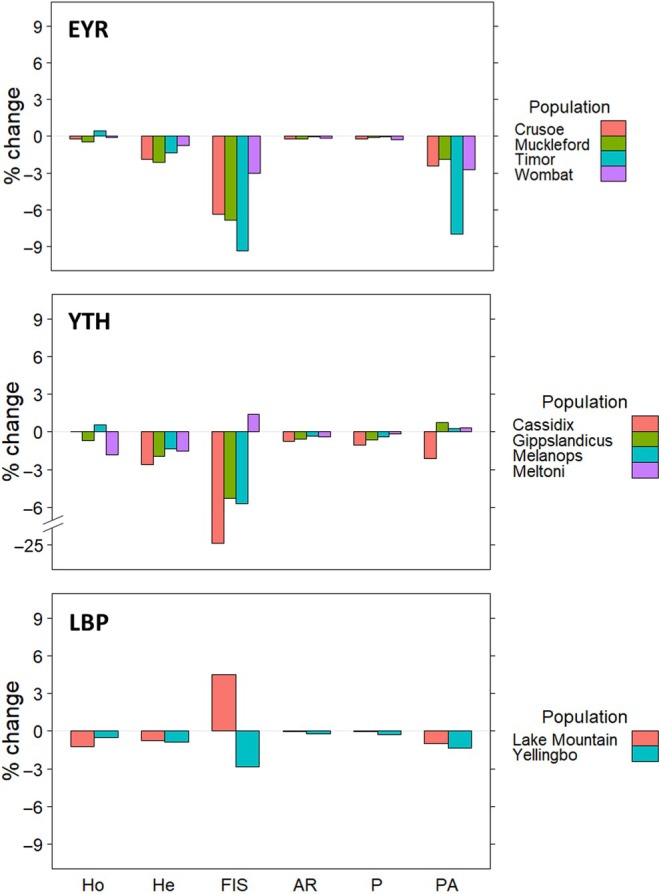
Percentage change of six measures of population genetic diversity after removing sex‐linked loci (AR, allelic richness; FIS, Wright's F _IS; He, expected heterozygosity; Ho, observed heterozygosity; P, polymorphism; PA, private alleles). Estimates are given per population of eastern yellow robin (EYR), yellow‐tufted honeyeater (YTH), and Leadbeater's possum (LBP).

3.5.2. Individual observed heterozygosity (Ho)

The removal of sex‐linked loci produced a statistically significant change in individual Ho, whose magnitude and direction varied between sexes and species (Table 4). For EYR, the decrease in female and male Ho was significant but small (F: 0.2% decrease, Cohen's D = 0.32; M: 0.3% decrease, Cohen's D = 0.42). For YTH, the change was an order of magnitude larger and went in opposite directions between the sexes: female Ho increased by 3.6% (p‐value < .001, Cohen's D = −9.1), and male Ho decreased by 3.0% (p‐value < .001, Cohen's D = 2.0). For LBP, the significant decrease was an order of magnitude larger for females (1.5%, p‐value < 0.001, Cohen's D = 1.7) than for males (0.2%, p‐value < .001, Cohen's D = 0.3). The opposite effect in male and female Ho translated into the disappearance of the significant (but misleading) difference between male and female Ho (mean difference = 5.13%, p‐value < .001) after the removal of sex‐linked loci from the YTH dataset (p‐value = .14; Table 5). There were no significant differences in Ho between the sexes in EYR and LBP before or after removing sex‐linked loci.

TABLE 4.

Paired t‐tests measuring the difference in individual observed heterozygosity (Ho) before and after removing sex‐linked loci, per sex, in each species. Results are presented for eastern yellow robin (EYR), yellow‐tufted honeyeater (YTH), and Leadbeater's possum (LBP). Significant p‐values are signalled in bold letters.

Sex	Mean before	Mean after	% change	Mean Δ	Δ SD	t statistic	df	p‐value	Cohen's D
EYR
F	0.188	0.188	−0.2%	−0.0003	0.0014	6.0	340	<.001	0.32
M	0.187	0.187	−0.3%	−0.0005	0.0015	8.6	411	<.001	0.42
YTH
F	0.156	0.161	3.6%	0.0056	0.0006	−152.8	280	<.001	−9.1
M	0.164	0.159	−3.0%	−0.0050	0.0025	37.2	338	<.001	2.0
LBP
F	0.172	0.169	−1.5%	−0.0026	0.0015	21.7	163	<.001	1.7
M	0.167	0.167	−0.2%	−0.0002	0.0009	4.1	211	<.001	0.28

TABLE 5.

t‐tests measuring the difference in individual observed heterozygosity (Ho) between females and males. Tests were done before and after removing sex‐linked loci, for eastern yellow robin (EYR), yellow‐tufted honeyeater (YTH), and Leadbeater's possum (LBP). Significant p‐values are signalled in bold letters.

	Mean females	Mean males	SE females	SE males	t statistic	df	p‐value	Cohen's D
EYR
Before	0.188	0.187	0.001	0.001	0.8	748.6	.45	0.05
After	0.188	0.187	0.001	0.001	0.9	749.9	.38	0.06
YTH
Before	0.156	0.164	0.001	0.001	−6.4	606.4	<.001	−0.5
After	0.162	0.159	0.001	0.001	1.5	613.9	.14	0.1
LBP
Before	0.172	0.167	0.003	0.003	1.1	343.9	.25	0.12
After	0.170	0.167	0.003	0.003	0.6	345.3	.55	0.06

3.5.3. Genetic structure

Before the removal of sex‐linked loci, PC1 explained 2.4% of the genetic variation in EYR, and divided the individuals into two groups (Crusoe‐Timor and Muckleford‐Wombat; Figure 7a). PC2, on the other hand, explained 1.6% of the variation and captured genetic structure due to the presence of sex‐linked loci: it divided the individuals into males and females (Figure 7b). This division between males and females disappeared from PC2 after removing sex‐linked loci (Figure 7c,d). For YTH and LBP, none of PC1, PC2, PC3 or PC4 showed sex genetic structure before or after using the function filter.sex.linked (Figures S6 and S7).

FIGURE 7.

Principal component analyses (PCA) of the genomic dataset of eastern yellow robin, EYR, before (top panels) and after (bottom panels) removing sex‐linked loci. In (a) and (c), individuals are coloured according to their population. In (b) and (d), individuals are coloured by sex.

3.5.4. Accuracy of parentage analyses

For EYR, before removing sex‐linked loci, an average of 3.83 runs out of five identified the correct parent. After removing sex‐linked loci, the average increased significantly to 4.19 (p‐value = .004; Table 6). We also found a significant association between the removal of sex‐linked loci and the number of correct final parentage assignments (χ ² = 4.8, df = 1, p‐value = .03): before removing sex‐linked loci, 91 out of 119 (76.5%) final assignments were correct, compared to 104 (87.4%) correct final assignments after removing sex‐linked loci. For YTH (cassidix), we found that removing sex‐linked loci did not significantly rise the average number of runs that correctly identified parents, which started with the high average of 4.9 runs (Table 6).

TABLE 6.

Paired t‐tests measuring the difference in the average number of COLONY runs (out of five) that identified the correct parent of an offspring before and after removing sex‐linked loci. Results are presented for eastern yellow robin (EYR) and yellow‐tufted honeyeater (YTH) subspecies cassidix. Significant p‐value is in bold.

Mean before	Mean after	% change	Mean Δ	Δ SD	t statistic	df	p‐value	Cohen's D
EYR
3.83	4.19	9.4%	0.36	1.3	−2.94	118	.004	−0.27
YTH (cassidix)
4.90	4.92	0.5%	0.02	0.4	0.28	39	.570	0.13

4. DISCUSSION

In this study, we developed and tested four R functions that automate tasks commonly needed in conservation genomic analyses: (1) filter.sex.linked to identify and remove sex‐linked loci, (2) infer.sex to infer the genetic sex of individuals using sex‐linked loci, (3) filter.excess.het to remove loci with abnormally high heterozygosity and (4) gl2colony to produce input files for parentage analysis software. Use of these functions on genomic data for two bird and one mammal species revealed that standard filters, such as low read depth and call rate, are inefficient at removing sex‐linked loci, removing fewer than half of Z‐linked/X‐linked loci and only 25%–50% of gametologs. In the three studied species, the failure to comprehensively remove sex‐linked loci led to one or more of: (i) overestimation of up to 24.4% of population F _IS, and up to 8% of the number of PA (ii) incorrectly inferring sex differences in individual heterozygosity, (iii) capturing sex genomic differences instead of population structure and (iv) inferring ~11% fewer parent‐offspring relationships in parentage analyses. We also found that function filter.sex.linked has over 98.8% accuracy for identifying autosomal loci when most individuals in a dataset are sexed, and that an initial set of 15 known males and 15 known females was enough to identify 88.7%–91.6% of all sex‐linked loci (through a preliminary run of function filter.sex.linked, followed by running function infer.sex and then re‐running function filter.sex.linked).

Appropriate filtering is a challenging part of population genomic analyses. It is widely acknowledged that filtering can significantly affect the inferences drawn from different analyses, ranging from ‘simple’ standard measures like heterozygosity, all the way to Genotype‐environment associations (e.g. Ahrens et al., 2021; Fu, 2014; Graham et al., 2020; Linck & Battey, 2019; Pearman et al., 2022; Shafer et al., 2017). Given this awareness, there is surprisingly little mention of best‐practices for filtering out sex‐linked loci from SNP datasets in population genomics research (but see Benestan et al., 2017; Trenkel et al., 2020). Unless using per‐marker F _ST or dartR's gl.report.sexlinked function to explicitly identify sex‐linked markers, studies rarely address them and seem to rely mainly on read depth and loci missing data filters to remove sex‐linked loci from large SNP datasets. We have demonstrated that this untargeted approach failed to remove ~20%–55% of all true sex‐linked loci (Figure 5). Filtering sex‐linked markers based only on assumed synteny with the sex chromosome of a heterospecific reference genome can also result in failing to account for neo‐sex chromosomes in evolutionary studies (Morales et al., 2018). Recent discoveries of neo‐sex chromosome systems in Sylvioidea (Sigeman et al., 2020, 2022), Australian robins (Gan et al., 2019), insects (Wang et al., 2022) and other systems highlight the dangers of assuming synteny with reference genomes of other species while detecting sex‐linked loci. Thus, we propose that the use of our filter.sex.linked function to remove sex‐linked loci before applying SNP quality filters can comprise best‐practice that will ensure that downstream filters are, in fact, evaluating the quality of autosomal loci.

We found that when most individuals on the dataset where correctly sexed, all or almost all of the candidate autosomal loci identified by function filter.sex.linked aligned to autosomes (i.e. the accuracy of function filter.sex.linked on identifying autosomal loci was 98.8%–100%). This points to the usefulness of the function in guaranteeing autosomal loci on which downstream population genetics analyses can be performed safely. On the other hand, a small proportion of candidate sex‐linked loci did not align with sex chromosomes but with autosomes (Table 2). There is the possibility, however, that the accuracy of the function in identifying W‐linked loci is higher than estimated (EYR = 93.2%, YTH = 92.3%; Table 2) because some unassembled scaffolds may belong to the W chromosome (the W chromosome is notorious for its difficulty in being assembled). The poorest performance of function filter.sex.linked was on diagnosing candidate gametologs for YTH (26.7% accuracy), which was much higher for EYR (94.3%). This is because the function wrongly identified as gametologs a small number of autosomal loci (YTH = 11 loci, EYR = 15 loci), and although these numbers were similar, they constituted a large proportion of the loci identified as gametologs in YTH (total = 17; four of them true ‘fixed’ gametologs, as predicted for species with old sex chromosomes), but not in EYR (total = 302; 248 of them true ‘fixed’ and ‘non‐fixed’ gametologs characteristic of neo‐sex chromosomes). Ultimately, we argue that although function filter.sex.linked may wrongly identify as sex‐linked a few autosomal loci, these loci are not “behaving” like autosomal loci in the dataset, and the safest approach is to remove them before downstream analyses of autosomal loci.

After testing the minimum requirements of functions filter.sex.linked and infer.sex, we found that 15 males and 15 females allowed the identification of the most true sex‐linked loci using a ‘loop run’ in the three species (Table 3). Importantly, ‘loop runs’ successfully removed most of the Z‐linked/X‐linked and gametologous loci, which are the ones that standard filters overwhelmingly fail to remove (Figure 5): they removed 100% in YTH, over 77% in EYR, and over 98.3% in LBP (Table 3). We also showed that, despite 15 males and 15 females allowing the initial identification of few sex‐linked loci, these loci permitted function infer.sex to make definite sex assignments with an accuracy that never dropped below 99%. Given that we tested our functions on three very different species—one bird with neo‐sex chromosomes, one bird with old sex chromosomes, and one marsupial mammal with proportionally short sex chromosomes (Gan et al., 2019; Graves, 2016; Marshall Graves & Shetty, 2001)—15 males and 15 females seem to be the minimum number of known‐sex individuals needed to perform a ‘loop run’. Nevertheless, this number may be larger for species with less variable sex chromosomes. Therefore, we recommend the use of at least 15 males and 15 females.

We showed that the failure to remove sex‐linked loci meant that a considerable proportion—3.8% and 6.6%—of the SNPs in the final EYR and YTH datasets were not autosomal and, therefore, yielded incorrect estimates of population diversity. Interestingly, this proportion was much smaller in LBP (0.9%) and still led to a 4.5% underestimation of Lake Mountain's FIS and a 2.8% overestimation of Yellingbo's (Figure 6). The effect of sex‐linked loci on genetic diversity biases varied among populations unpredictably and was not influenced by the within‐population sex ratio (Figure 6). This is likely because there are many factors intervening in addition to sample sex‐bias, such as different allelic frequencies of sex‐linked loci in the populations, the total amount of sex‐linked versus autosomal loci (that may vary between populations due to genotyping error), the sex‐chromosome‐to‐autosome diversity ratio (due to different selective pressures and levels of genetic drift), and the level of recombination between sex chromosomes. This highlights the necessity of searching for and carefully filtering out sex‐linked loci because it would be hard to control for their presence in other ways (e.g. by introducing sample sex ratio in statistical models).

Despite the relatively small impact of the presence of sex‐linked loci on population Ho, there was a significant impact on individual Ho that was large enough to erroneously indicate that YTH females were 5.1% less heterozygous than males (Table 5). This spurious significant difference could have mistakenly suggested that females are philopatric (which is not true in cassidix; Smales, 2004) or that they experience less inbreeding depression for survival (the reverse is true in cassidix; Harrisson et al., 2019). If these hypotheses were not known in advance to be incorrect, they might have been accepted or at least further investigated; thus, poor filtering of sex‐linked loci can lead to incorrect ecological and evolutionary inferences and wasted resources.

Our results also illustrated how the presence of sex‐linked SNPs can obscure population structure. The first PC on EYR data showed population structure due to geographically separated groups. The second PC, however, simply captured the genetic differences between sexes when sex‐linked markers were not removed, obscuring the fact that in reality, the second largest source of genetic variation comes from within the Muckleford population (Figure 7). This masking of population structure has also been observed in the Discriminant Analysis of Principal Components (DAPC) of two species of lobsters due to the presence of a few sex‐linked loci (Benestan et al., 2017). If not properly checked against sex, the PC2 split in two could have been interpreted as, for instance, the presence of two cryptic sympatric species. Researchers studying populations with little genetic variation should be particularly careful, because this effect is expected to be more pronounced for populations with low genetic differentiation.

Importantly, we found that failing to remove sex‐linked loci led to ~11% fewer correct parentage assignments for EYR. Such a substantial loss of correct assignments could have repercussions for the management of endangered species. For example, releases of captive‐bred individuals or translocations/introductions are usually done avoiding the release of close relatives in the same group in order to maximise genetic diversity and discourage inbreeding (e.g. cassidix; Frankham et al., 2017; Harrisson et al., 2016). Removing sex‐linked loci will be even more crucial in the absence of a set of known parentages with which to calibrate parentage analyses as is likely to apply to many species of conservation concern such as (i) those whose breeding season cannot be monitored because it occurs in inaccessible locations or because of lack of resources, (ii) polygamous and cooperative‐breeding species, (iii) those with external fertilisation like amphibian and fish species (Nakamura, 2009). Accounting for sex‐linked loci is also likely to have the largest impact on species with large sex chromosomes (including neo‐sex chromosomes, which have been discovered in many taxa including EYR) because sex‐linked loci will represent a large proportion of the potential genomic markers for parentage analysis (Beukeboom & Perrin, 2014; Gan et al., 2019; Sigeman et al., 2022).

The functions we propose were created with the needs of conservation genomicists and wildlife managers in mind. Function filter.sex.linked requires, in essence, just a SNP matrix and at least 30 sexed individuals. Sexing individuals is especially important for species without sex dimorphism or for sexually dimorphic species whose youngs' sex is undistinguishable. With the combination of the functions filter.sex.linked and infer.sex, we offer a formal statistical framework that systematically identifies and uses sex‐linked loci to make sex assignments with as few as 15 known‐sex individuals of each sex. Unlike current practices, function infer.sex was designed to use the complementary information contained in all types of sex‐linked loci available, which makes the sex assignments more accurate (Figure 4d–f). The use of all types of sex‐linked loci will be advantageous for low‐density marker datasets because it uses information that would otherwise be neglected, and it facilitates the development of SNP panels that include sex‐specific loci (Blåhed et al., 2018; Willis et al., 2020). It also allows for error‐checking and confirming congruence between genetic and phenotypic sex of individuals, which may assist in detecting cases of environmental sex‐reversal (Stelkens & Wedekind, 2010). The separation of sex‐linked loci can be used to validate the assembly of W and Y chromosomes and to study sex‐specific processes (e.g. natural selection and philopatry). Furthermore, it reduces the cost in time, genetic material and resources of using other sexing methods (e.g. PCR amplification of CHD1‐Z and CHD1‐W genes; Fridolfsson & Ellegren, 1999).

The function filter.excess.het provides a statistically‐backed method to identify artefactual multilocus SNPs that show abnormally high heterozygosity. The function circumvents the problem of choosing an arbitrary heterozygosity threshold by, instead, testing loci whose heterozygosity ≥0.5 and also have a significant excess of heterozygotes beyond sampling error. This has the advantage of taking into account random sampling and genotyping errors that affect loci differently. In fact, this approach is available in VCFtools but not yet in dartR, snpR or SNPfiltR (Danecek et al., 2011; DeRaad, 2022; Hemstrom & Jones, 2023; Hohenlohe et al., 2011; Mijangos et al., 2022). Nonetheless, we would like to emphasise that this is not a Hardy–Weinberg equilibrium filter (which requires critical thinking to be correctly applied and interpreted; Waples, 2015) because it does not remove all loci that deviate from Hardy–Weinberg proportions (only those whose heterozygosity ≥0.5). This function should be used only when looking to obtain neutral autosomal loci (cf. looking for signatures of selection).

In conclusion, we demonstrated how incomplete removal of sex‐linked loci can bias conservation genomic inferences. We argue that comprehensively removing sex‐linked loci should be best‐practice when handling genomic data, and we offer convenient, easy‐to‐use resources to automate this and other bioinformatic steps. The functions presented here can be integrated into bioinformatic pipelines and widely used R packages such as dartR, sambaR, SNPfiltR and snpR. By developing functions that can be easily adopted by conservation biologists and incorporated into wildlife management workflows, this study will contribute to a better understanding of the processes occurring in threatened species, such as inbreeding, inbreeding depression and population structure.

AUTHOR CONTRIBUTIONS

Diana A. Robledo‐Ruiz, Alexandra Pavlova and Paul Sunnucks led the initial project conceptualization and design. Lana Austin, J. Nevil Amos and Daniel K. P. Harley collected EYR and LBP field samples and genotyping data and conducted initial analyses of sex‐linked loci. Diana A. Robledo‐Ruiz and Jesús Castrejón‐Figueroa wrote the R functions and analysed the data with guidance from Paul Sunnucks and Alexandra Pavlova. Alexandra Pavlova and Diana A. Robledo‐Ruiz wrote the first draft of the manuscript, and all authors contributed to editing and writing. All authors approved the final version of this manuscript for publication. Paul Sunnucks, Alexandra Pavlova, Michael J. L. Magrath and Lana Austin secured funding for the project.

CONFLICT OF INTEREST STATEMENT

The authors declare no conflicts of interest to declare.

BENEFIT‐SHARING STATEMENT

The contributions of all individuals to the research, including volunteers, are described in the Acknowledgements. The results of this research have been shared with stakeholders and the broader scientific community. Benefits from this research accrue from the sharing of our data and results on public databases as described above.

Supporting information

Data S1

Robledo‐Ruiz, D. A. , Austin, L. , Amos, J. N. , Castrejón‐Figueroa, J. , Harley, D. K. P. , Magrath, M. J. L. , Sunnucks, P. , & Pavlova, A. (2025). Easy‐to‐use R functions to separate reduced‐representation genomic datasets into sex‐linked and autosomal loci, and conduct sex assignment. Molecular Ecology Resources, 25, e13844. 10.1111/1755-0998.13844

DATA AVAILABILITY STATEMENT

The R functions are available at https://github.com/drobledoruiz/conservation_genomics. All data and scripts used in this manuscript have been archived in Bridges Monash University research repository at https://doi.org/10.26180/21608028.v6 (Robledo Ruiz et al., 2022).

REFERENCES

- Ahrens, C. W. , Jordan, R. , Bragg, J. , Harrison, P. A. , Hopley, T. , Bothwell, H. , & Rymer, P. D. (2021). Regarding the F‐word: The effects of data filtering on inferred genotype‐environment associations. Molecular Ecology Resources, 21(5), 1460–1474. [DOI] [PubMed] [Google Scholar]
- Allendorf, F. W. , Funk, W. C. , Aitken, S. N. , Byrne, M. , & Luikart, G. (2022). Conservation and the genomics of populations. Oxford University Press. [DOI] [PMC free article] [PubMed] [Google Scholar]
- Altschul, S. F. , Gish, W. , Miller, W. , Myers, E. W. , & Lipman, D. J. (1990). Basic local alignment search tool. Journal of Molecular Biology, 215(3), 403–410. [DOI] [PubMed] [Google Scholar]
- Amos, J. N. , Harrisson, K. A. , Radford, J. Q. , White, M. , Newell, G. , Mac Nally, R. , Sunnucks, P. , & Pavlova, A. (2014). Species‐ and sex‐specific connectivity effects of habitat fragmentation in a suite of woodland birds. Ecology, 95, 1556–1568. [DOI] [PubMed] [Google Scholar]
- Arnold, B. D. , & Wilkinson, G. S. (2015). Female natal philopatry and gene flow between divergent clades of pallid bats (Antrozous pallidus). Journal of Mammalogy, 96(3), 531–540. [Google Scholar]
- Baird, N. A. , Etter, P. D. , Atwood, T. S. , Currey, M. C. , Shiver, A. L. , Lewis, Z. A. , Selker, E. U. , Cresko, W. A. , & Johnson, E. A. (2008). Rapid SNP discovery and genetic mapping using sequenced RAD markers. PLoS ONE, 3(10), e3376. [DOI] [PMC free article] [PubMed] [Google Scholar]
- Benjamini, Y. , & Hochberg, Y. (1995). Controlling the false discovery rate: A practical and powerful approach to multiple testing. Journal of the Royal Statistical Society, Series B, 57, 289–300. [Google Scholar]
- Benestan, L. , Moore, J. S. , Sutherland, B. J. , Le Luyer, J. , Maaroufi, H. , Rougeux, C. , Normandeau, L. , Rycroft, N. , Atema, J. , Harris, L. N. , Tallman, R. F. , Greenwood, S. J. , Clark, F. K. , & Bernatchez, L. (2017). Sex matters in massive parallel sequencing: Evidence for biases in genetic parameter estimation and investigation of sex determination systems. Molecular Ecology, 26(24), 6767–6783. [DOI] [PubMed] [Google Scholar]
- Beukeboom, L. W. , & Perrin, N. (2014). The evolution of sex determination. Oxford University Press. [Google Scholar]
- Blåhed, I. M. , Königsson, H. , Ericsson, G. , & Spong, G. (2018). Discovery of SNPs for individual identification by reduced representation sequencing of moose (Alces alces). PLoS ONE, 13(5), e0197364. [DOI] [PMC free article] [PubMed] [Google Scholar]
- Britt, M. , Haworth, S. E. , Johnson, J. B. , Martchenko, D. , & Shafer, A. B. (2018). The importance of non‐academic coauthors in bridging the conservation genetics gap. Biological Conservation, 218, 118–123. [Google Scholar]
- Carvalho, A. B. , & Clark, A. G. (2013). Efficient identification of Y chromosome sequences in the human and drosophila genomes. Genome Research, 23(11), 1894–1907. [DOI] [PMC free article] [PubMed] [Google Scholar]
- Castella, V. , Ruedi, M. , & Excoffier, L. (2001). Contrasted patterns of mitochondrial and nuclear structure among nursery colonies of the bat Myotis myotis . Journal of Evolutionary Biology, 14(5), 708–720. [Google Scholar]
- Chen, N. , Van Hout, C. V. , Gottipati, S. , & Clark, A. G. (2014). Using Mendelian inheritance to improve high‐throughput SNP discovery. Genetics, 198(3), 847–857. [DOI] [PMC free article] [PubMed] [Google Scholar]
- Danecek, P. , Auton, A. , Abecasis, G. , Albers, C. A. , Banks, E. , DePristo, M. A. , & 1000 Genomes Project Analysis Group . (2011). The variant call format and VCFtools. Bioinformatics, 27(15), 2156–2158. [DOI] [PMC free article] [PubMed] [Google Scholar]
- Davey, J. W. , & Blaxter, M. L. (2010). RADSeq: Next‐generation population genetics. Briefings in Functional Genomics, 9(5–6), 416–423. [DOI] [PMC free article] [PubMed] [Google Scholar]
- de Jong, M. J. , de Jong, J. F. , Hoelzel, A. R. , & Janke, A. (2021). SambaR: An R package for fast, easy and reproducible population‐genetic analyses of biallelic SNP data sets. Molecular Ecology Resources, 21(4), 1369–1379. [DOI] [PubMed] [Google Scholar]
- DeRaad, D. A. (2022). SNPfiltR: An R package for interactive and reproducible SNP filtering. Molecular Ecology Resources, 22, 2443–2453. [DOI] [PubMed] [Google Scholar]
- Drinan, D. P. , Loher, T. , & Hauser, L. (2018). Identification of genomic regions associated with sex in Pacific halibut. Journal of Heredity, 109(3), 326–332. [DOI] [PubMed] [Google Scholar]
- Dudchenko, O. , Batra, S. S. , Omer, A. D. , Nyquist, S. K. , Hoeger, M. , Durand, N. C. , Shamim, M. S. , Machol, I. , Lander, E. S. , Aiden, A. P. , & Aiden, E. L. (2017). De novo assembly of the Aedes aegypti genome using Hi‐C yields chromosome‐length scaffolds. Science, 356(6333), 92–95. 10.1126/science.aal3327 [DOI] [PMC free article] [PubMed] [Google Scholar]
- Dudchenko, O. , Shamim, M. S. , Batra, S. S. , Durand, N. C. , Musial, N. T. , Mostofa, R. , Pham, M. , Hilaire, B. G. S. , Yao, W. , Stamenova, E. , Hoeger, M. , Nyquist, S. K. , Korchina, V. , Pletch, K. , Flanagan, J. P. , Tomaszewicz, A. , McAloose, D. , Estrada, C. P. , Novak, B. J. , … Aiden, E. L. (2018). The Juicebox Assembly Tools module facilitates de novo assembly of mammalian genomes with chromosome‐length scaffolds for under $1000. BioRxiv, 254797. 10.1101/254797 [DOI]
- Ellegren, H. (2009). The different levels of genetic diversity in sex chromosomes and autosomes. Trends in Genetics, 25(6), 278–284. [DOI] [PubMed] [Google Scholar]
- Ellegren, H. (2014). Genome sequencing and population genomics in non‐model organisms. Trends in Ecology & Evolution, 29(1), 51–63. [DOI] [PubMed] [Google Scholar]
- Feron, R. , Pan, Q. , Wen, M. , Imarazene, B. , Jouanno, E. , Anderson, J. , & Guiguen, Y. (2021). RADSex: A computational workflow to study sex determination using restriction site‐associated DNA sequencing data. Molecular Ecology Resources, 21(5), 1715–1731. [DOI] [PMC free article] [PubMed] [Google Scholar]
- Fitzpatrick, S. W. , Bradburd, G. S. , Kremer, C. T. , Salerno, P. E. , Angeloni, L. M. , & Funk, W. C. (2020). Genomic and fitness consequences of genetic rescue in wild populations. Current Biology, 30(3), 517–522. [DOI] [PubMed] [Google Scholar]
- Flanagan, S. P. , & Jones, A. G. (2019). The future of parentage analysis: From microsatellites to SNPs and beyond. Molecular Ecology, 28(3), 544–567. [DOI] [PubMed] [Google Scholar]
- Frankham, R. , Ballou, J. D. , Ralls, K. , Eldridge, M. , Dudash, M. R. , Fenster, C. B. , Lacy, R. C. , & Sunnucks, P. (2017). Genetic management of fragmented animal and plant populations. Oxford University Press. [Google Scholar]
- Fridolfsson, A. K. , & Ellegren, H. (1999). A simple and universal method for molecular sexing of non‐ratite birds. Journal of Avian Biology, 30, 116–121. [Google Scholar]
- Fu, Y. B. (2014). Genetic diversity analysis of highly incomplete SNP genotype data with imputations: An empirical assessment. G3: Genes, Genomes, Genetics, 4(5), 891–900. 10.1534/g3.114.010942 [DOI] [PMC free article] [PubMed] [Google Scholar]
- Galla, S. J. , Brown, L. , Couch‐Lewis, Y. , Cubrinovska, I. , Eason, D. , Gooley, R. M. , Hamilton, J. A. , Heath, J. A. , Hauser, S. S. , Latch, E. K. , Matocq, M. D. , Richardson, A. , Wold, J. R. , Hogg, C. J. , Santure, A. W. , & Steeves, T. E. (2022). The relevance of pedigrees in the conservation genomics era. Molecular Ecology Resources, 31(1), 41–54. 10.1111/mec.16192 [DOI] [PMC free article] [PubMed] [Google Scholar]
- Galla, S. J. , Buckley, T. R. , Elshire, R. , Hale, M. L. , Knapp, M. , McCallum, J. , Moraga, R. , Santure, A. W. , Wilcox, P. , & Steeves, T. E. (2016). Building Strong Relationships between Conservation Genetics and Primary Industry Leads to Mutually Beneficial Genomic Advances. Molecular Ecology, 25, 5267–5281. 10.1111/mec.13837 [DOI] [PubMed] [Google Scholar]
- Gan, H. M. , Falk, S. , Morales, H. E. , Austin, C. M. , Sunnucks, P. , & Pavlova, A. (2019). Genomic evidence of neo‐sex chromosomes in the eastern yellow robin. GigaScience, 8(9), giz111. [DOI] [PMC free article] [PubMed] [Google Scholar]
- Goudet, J. (2005). Hierfstat, a package for R to compute and test hierarchical F‐statistics. Molecular Ecology Notes, 5(1), 184–186. [Google Scholar]
- Graham, C. F. , Boreham, D. R. , Manzon, R. G. , Stott, W. , Wilson, J. Y. , & Somers, C. M. (2020). How “simple” methodological decisions affect interpretation of population structure based on reduced representation library DNA sequencing: A case study using the lake whitefish. PLoS ONE, 15(1), e0226608. [DOI] [PMC free article] [PubMed] [Google Scholar]
- Graves, J. A. (2016). Did sex chromosome turnover promote divergence of the major mammal groups? De novo sex chromosomes and drastic rearrangements may have posed reproductive barriers between monotremes, marsupials and placental mammals. BioEssays, 38(8), 734–743. [DOI] [PMC free article] [PubMed] [Google Scholar]
- Gruber, B. , Unmack, P. , Berry, O. , & Georges, A. (2019). Introduction to dartR . User Manual 51.
- Gruber, B. , Unmack, P. J. , Berry, O. F. , & Georges, A. (2018). dartr: An r package to facilitate analysis of SNP data generated from reduced representation genome sequencing. Molecular Ecology Resources, 18(3), 691–699. [DOI] [PubMed] [Google Scholar]
- Hansen, B. D. , Harley, D. K. , Lindenmayer, D. B. , & Taylor, A. C. (2009). Population genetic analysis reveals a long‐term decline of a threatened endemic Australian marsupial. Molecular Ecology, 18(16), 3346–3362. [DOI] [PubMed] [Google Scholar]
- Harrisson, K. A. , Magrath, M. J. , Yen, J. D. , Pavlova, A. , Murray, N. , Quin, B. , Menkhorst, P. , Miller, K. A. , Cartwright, K. , & Sunnucks, P. (2019). Lifetime fitness costs of inbreeding and being inbred in a critically endangered bird. Current Biology, 29, 2711–2717. [DOI] [PubMed] [Google Scholar]
- Harrisson, K. A. , Pavlova, A. , Gonçalves da Silva, A. , Rose, R. , Bull, J. K. , Lancaster, M. L. , Murray, N. , Quin, B. , Menkhorst, P. , Magrath, M. J. , & Sunnucks, P. (2016). Scope for genetic rescue of an endangered subspecies though re‐establishing natural gene flow with another subspecies. Molecular Ecology, 25(6), 1242–1258. 10.1111/mec.13547 [DOI] [PubMed] [Google Scholar]
- Hemstrom, W. , & Jones, M. (2023). snpR: User friendly population genomics for SNP data sets with categorical metadata. Molecular Ecology Resources, 23(4), 962–973. [DOI] [PubMed] [Google Scholar]
- Hoffmann, A. , Griffin, P. , Dillon, S. , Catullo, R. , Rane, R. , Byrne, M. , Jordan, R. , Oakeshott, J. , Weeks, A. , Joseph, L. , Lockhart, P. , Borevitz, J. , & Sgrò, C. (2015). A framework for incorporating evolutionary genomics into biodiversity conservation and management. Climate Change Responses, 2(1), 1–24. 10.1186/s40665-014-0009-x [DOI] [Google Scholar]
- Hogg, C. J. , Ottewell, K. , Latch, P. , Rossetto, M. , Biggs, J. , Gilbert, A. , Richmond, S. , & Belov, K. (2022). Threatened Species Initiative: Empowering conservation action using genomic resources. Proceedings of the National Academy of Sciences of the United States of America, 119(4), e2115643118. 10.1073/pnas.2115643118 [DOI] [PMC free article] [PubMed] [Google Scholar]
- Hohenlohe, P. A. , Amish, S. J. , Catchen, J. M. , Allendorf, F. W. , & Luikart, G. (2011). Next‐generation RAD sequencing identifies thousands of SNPs for assessing hybridization between rainbow and westslope cutthroat trout. Molecular Ecology Resources, 11, 117–122. [DOI] [PubMed] [Google Scholar]
- Hohenlohe, P. A. , Funk, W. C. , & Rajora, O. P. (2021). Population genomics for wildlife conservation and management. Molecular Ecology, 30(1), 62–82. [DOI] [PMC free article] [PubMed] [Google Scholar]
- Holderegger, R. , Balkenhol, N. , Bolliger, J. , Engler, J. O. , Gugerli, F. , Hochkirch, A. , Nowak, C. , Segelbacher, G. , Widmer, A. , & Zachos, F. E. (2019). Conservation genetics: Linking science with practice. Molecular Ecology, 28(17), 3848–3856. [DOI] [PubMed] [Google Scholar]
- Jombart, T. , & Ahmed, I. (2011). adegenet 1.3‐1: New tools for the analysis of genome‐wide SNP data. Bioinformatics, 27(21), 3070–3071. [DOI] [PMC free article] [PubMed] [Google Scholar]
- Jones, O. R. , & Wang, J. (2010). COLONY: A program for parentage and sibship inference from multilocus genotype data. Molecular Ecology Resources, 10(3), 551–555. [DOI] [PubMed] [Google Scholar]
- Käfer, J. , Lartillot, N. , Marais, G. A. , & Picard, F. (2021). Detecting sex‐linked genes using genotyped individuals sampled in natural populations. Genetics, 218(2), iyab053. [DOI] [PMC free article] [PubMed] [Google Scholar]
- Kardos, M. (2021). Conservation genetics. Current Biology, 31(19), R1185–R1190. [DOI] [PubMed] [Google Scholar]
- Kilian, A. , Wenzl, P. , Huttner, E. , Carling, J. , Xia, L. , Blois, H. , Caig, V. , Heller‐Uszynska, K. , Jaccoud, D. , Hopper, C. , Aschenbrenner‐Kilian, M. , Evers, M. , Peng, K. , Cayla, C. , Hok, P. , & Uszynski, G. (2012). Diversity arrays technology: A generic genome profiling technology on open platforms. In Pompanon F. & Bonin A. (Eds.), Data production and analysis in population genomics (pp. 67–89). Humana Press. [DOI] [PubMed] [Google Scholar]
- Linck, E. , & Battey, C. J. (2019). Minor allele frequency thresholds strongly affect population structure inference with genomic data sets. Molecular Ecology Resources, 19(3), 639–647. [DOI] [PubMed] [Google Scholar]
- Marshall Graves, J. A. , & Shetty, S. (2001). Sex from W to Z: Evolution of vertebrate sex chromosomes and sex determining genes. Journal of Experimental Zoology, 290(5), 449–462. [DOI] [PubMed] [Google Scholar]
- McMahon, B. J. , Teeling, E. C. , & Höglund, J. (2014). How and why should we implement genomics into conservation? Evolutionary applications, 7(9), 999–1007. [DOI] [PMC free article] [PubMed] [Google Scholar]
- Mijangos, J. L. , Gruber, B. , Berry, O. , Pacioni, C. , & Georges, A. (2022). dartR v2: An accessible genetic analysis platform for conservation, ecology and agriculture. Methods in Ecology and Evolution, 13, 2150–2158. [Google Scholar]
- Morales, H. E. , Pavlova, A. , Amos, N. , Major, R. , Killian, A. , Greening, C. , & Sunnucks, P. (2018). Concordant divergence of mitogenomes and a mitonuclear gene cluster in bird lineages inhabiting different climates. Nature Ecology and Evolution, 2, 1258–1267. [DOI] [PubMed] [Google Scholar]
- Moran, B. M. , Thomas, S. M. , Judson, J. M. , Navarro, A. , Davis, H. , Sidak‐Loftis, L. , Korody, M. , Mace, M. , Ralls, K. , Callicrate, T. , Ryder, O. A. , Chemnick, L. G. , & Steiner, C. C. (2021). Correcting parentage relationships in the endangered California Condor: Improving mean kinship estimates for conservation management. The Condor, 123(3), duab017. 10.1093/ornithapp/duab017 [DOI] [Google Scholar]
- Mucci, N. , Giangregorio, P. , Cirasella, L. , Isani, G. , & Mengoni, C. (2020). A new STR panel for parentage analysis in endangered tortoises. Conservation Genetics Resources, 12(1), 67–75. [Google Scholar]
- Nakamura, M. (2009). Sex determination in amphibians. Seminars in Cell & Developmental Biology, 20(3), 271–282. [DOI] [PubMed] [Google Scholar]
- Nursyifa, C. , Brüniche‐Olsen, A. , Garcia‐Erill, G. , Heller, R. , & Albrechtsen, A. (2022). Joint identification of sex and sex‐linked scaffolds in non‐model organisms using low depth sequencing data. Molecular Ecology Resources, 22(2), 458–467. [DOI] [PubMed] [Google Scholar]
- O'Leary, S. J. , Puritz, J. B. , Willis, S. C. , Hollenbeck, C. M. , & Portnoy, D. S. (2018). These aren't the loci you'e looking for: Principles of effective SNP filtering for molecular ecologists. Molecular Ecology, 27, 3193–3206. 10.1111/mec.14792 [DOI] [PubMed] [Google Scholar]
- Overbeek, A. , Galla, S. , Brown, L. , Cleland, S. , Thyne, C. , Maloney, R. , & Steeves, T. (2020). Pedigree validation using genetic markers in an intensively‐managed taonga species, the critically endangered kaki (Himantopus novaezelandiae). Notornis, 67(4), 709–716. [Google Scholar]
- Pavlova, A. , Amos, J. N. , Joseph, L. , Loynes, K. , Austin, J. J. , Keogh, J. S. , Stone, G. , Nicholls, J. A. , & Sunnucks, P. (2013). Perched at the mito‐nuclear crossroads: Divergent mitochondrial lineages correlate with environment in the face of ongoing nuclear gene flow in an Australian bird. Evolution, 67, 3412–3428. 10.1111/evo.12107 [DOI] [PubMed] [Google Scholar]
- Pavlova, A. , Harrisson, K. A. , Turakulov, R. , Lee, Y. P. , Ingram, B. A. , Gilligan, D. , Sunnucks, P. , & Gan, H. M. (2022). Labile sex chromosomes in the Australian freshwater fish family Percichthyidae. Molecular Ecology Resources, 22(4), 1639–1655. 10.1111/1755-0998.13569 [DOI] [PubMed] [Google Scholar]
- Pavlova, A. , Selwood, P. , Harrisson, K. A. , Murray, N. , Quin, B. , Menkhorst, P. , Smales, I. , & Sunnucks, P. (2014). Integrating phylogeography and morphometrics to assess conservation merits and inform conservation strategies for an endangered subspecies of a common bird species. Biological Conservation, 174, 136–146. [Google Scholar]
- Pearman, W. S. , Urban, L. , & Alexander, A. (2022). Commonly used Hardy–Weinberg equilibrium filtering schemes impact population structure inferences using RADseq data. Molecular Ecology Resources, 22(7), 2599–2613. [DOI] [PMC free article] [PubMed] [Google Scholar]
- Peneder, P. , Wallner, B. , & Vogl, C. (2017). Exchange of genetic information between therian X and Y chromosome gametologs in old evolutionary strata. Ecology and Evolution, 7(20), 8478–8487. [DOI] [PMC free article] [PubMed] [Google Scholar]
- Peterson, B. K. , Weber, J. N. , Kay, E. H. , Fisher, H. S. , & Hoekstra, H. E. (2012). Double digest RADseq: An inexpensive method for de novo SNP discovery and genotyping in model and non‐model species. PLoS ONE, 7(5), e37135. [DOI] [PMC free article] [PubMed] [Google Scholar]
- Pritchard, J. K. , Stephens, M. , & Donnelly, P. (2000). Inference of population structure using multilocus genotype data. Genetics, 155(2), 945–959. [DOI] [PMC free article] [PubMed] [Google Scholar]
- R Core Team . (2022). R: A language and environment for statistical computing. R Foundation for Statistical Computing. https://www.R‐project.org/ [Google Scholar]
- Radosavljević, I. , Satovic, Z. , & Liber, Z. (2015). Causes and consequences of contrasting genetic structure in sympatrically growing and closely related species. AoB Plants, 7, lv106. 10.1093/aobpla/plv106 [DOI] [PMC free article] [PubMed] [Google Scholar]
- Robledo Ruiz, D. , Pavlova, A. , & Sunnucks, P. (2022). Supporting data for Robledo‐Ruiz et al. (2023). Monash University. Dataset. 10.26180/21608028.v6 [DOI]
- Robledo‐Ruiz, D. A. , Gan, H. M. , Kaur, P. , Dudchenko, O. , Weisz, D. , Khan, R. , Lieberman Aiden, E. , Osipova, E. , Hiller, M. , Morales, H. E. , Magrath, M. J. L. , Clarke, R. H. , Sunnucks, P. , & Pavlova, A. (2022). Chromosome‐length genome assembly and linkage map of a critically endangered Australian bird: The helmeted honeyeater. GigaScience, 11, giac025. 10.1093/gigascience/giac025 [DOI] [PMC free article] [PubMed] [Google Scholar]
- Robledo‐Ruiz, D. A. , Pavlova, A. , Clarke, R. H. , Magrath, M. J. , Quin, B. , Harrisson, K. A. , Gan, H. M. , Low, G. W. , & Sunnucks, P. (2022). A novel framework for evaluating in situ breeding management strategies in endangered populations. Molecular Ecology Resources, 22(1), 239–253. 10.1111/1755-0998.13476 [DOI] [PubMed] [Google Scholar]
- Shafer, A. B. A. , Peart, C. R. , Tusso, S. , Maayan, I. , Brelsford, A. , Wheat, C. W. , & Wolf, J. B. W. (2017). Bioinformatic processing of RAD‐seq data dramatically impacts downstream population genetic inference. Methods in Ecology and Evolution, 8(8), 907–917. [Google Scholar]
- Sigeman, H. , Ponnikas, S. , & Hansson, B. (2020). Whole‐genome analysis across 10 songbird families within Sylvioidea reveals a novel autosome–sex chromosome fusion. Biology Letters, 16, 20200082. [DOI] [PMC free article] [PubMed] [Google Scholar]
- Sigeman, H. , Zhang, H. , Ali Abed, S. , & Hansson, B. (2022). A novel neo‐sex chromosome in Sylvietta brachyura (Macrosphenidae) adds to the extraordinary avian sex chromosome diversity among Sylvioidea songbirds. Journal of Evolutionary Biology, 35, 1797–1805. [DOI] [PMC free article] [PubMed] [Google Scholar]
- Smales, I. J. (2004). Population ecology of the helmeted honeyeater Lichenostomus melanops cassidix: Long‐term investigations of a threatened bird (Doctoral dissertation). University of Melbourne, School of Botany. [Google Scholar]
- Stelkens, R. B. , & Wedekind, C. (2010). Environmental sex reversal, Trojan sex genes, and sex ratio adjustment: Conditions and population consequences. Molecular Ecology, 19(4), 627–646. [DOI] [PubMed] [Google Scholar]
- Taylor, H. R. , Dussex, N. , & van Heezik, Y. (2017). Bridging the conservation genetics gap by identifying barriers to implementation for conservation practitioners. Global Ecology and Conservation, 10, 231–242. [Google Scholar]
- Trenkel, V. M. , Boudry, P. , Verrez‐Bagnis, V. , & Lorance, P. (2020). Methods for identifying and interpreting sex‐linked SNP markers and carrying out sex assignment: Application to thornback ray (Raja clavata). Molecular Ecology Resources, 20(6), 1610–1619. [DOI] [PubMed] [Google Scholar]
- Van Rossum, F. (2022). Sibship and parentage reconstruction as a genetic tool for designing and monitoring plant translocations. Restoration Ecology, 31, e13726. 10.1111/rec.13726 [DOI] [Google Scholar]
- Wang, S. , Nalley, M. J. , Chatla, K. , Aldaimalani, R. , MacPherson, A. , Wei, K. H. C. , Corbett‐Detig, R. B. , Mai, D. , & Bachtrog, D. (2022). Neo‐sex chromosome evolution shapes sex‐dependent asymmetrical introgression barrier. Proceedings of the National Academy of Sciences of the United States of America, 119(19), e2119382119. 10.1073/pnas.2119382119 [DOI] [PMC free article] [PubMed] [Google Scholar]
- Waples, R. S. (2015). Testing for hardy–Weinberg proportions: Have we lost the plot? Journal of Heredity, 106(1), 1–19. [DOI] [PubMed] [Google Scholar]
- Willi, Y. , Kristensen, T. N. , Sgrò, C. M. , Weeks, A. R. , Ørsted, M. , & Hoffmann, A. A. (2022). Conservation genetics as a management tool: The five best‐supported paradigms to assist the management of threatened species. Proceedings of the National Academy of Sciences of the United States of America, 119(1), e2105076119. [DOI] [PMC free article] [PubMed] [Google Scholar]
- Willis, S. C. , Hess, J. E. , Fryer, J. K. , Whiteaker, J. M. , Brun, C. , Gerstenberger, R. , & Narum, S. R. (2020). Steelhead (Oncorhynchus mykiss) lineages and sexes show variable patterns of association of adult migration timing and age‐at‐maturity traits with two genomic regions. Evolutionary Applications, 13(10), 2836–2856. [DOI] [PMC free article] [PubMed] [Google Scholar]
- Willis, S. C. , Hollenbeck, C. M. , Puritz, J. B. , Gold, J. R. , & Portnoy, D. S. (2017). Haplotyping RAD loci: An efficient method to filter paralogs and account for physical linkage. Molecular Ecology Resources, 17(5), 955–965. [DOI] [PubMed] [Google Scholar]
- Woinarski, J. , & Burbidge, A. A. (2016). Gymnobelideus leadbeateri . The IUCN Red List of Threatened Species.
- Zilko, J. P. , Harley, D. , Hansen, B. , Pavlova, A. , & Sunnucks, P. (2020). Accounting for cryptic population substructure enhances detection of inbreeding depression with genomic inbreeding coefficients: An example from a critically endangered marsupial. Molecular Ecology, 29(16), 2978–2993. [DOI] [PubMed] [Google Scholar]
- Zilko, J. P. , Harley, D. , Pavlova, A. , & Sunnucks, P. (2021). Applying population viability analysis to inform genetic rescue that preserves locally unique genetic variation in a critically endangered mammal. Diversity, 13(8), 382. [Google Scholar]
Associated Data
This section collects any data citations, data availability statements, or supplementary materials included in this article.
Supplementary Materials