Discrete Representation Learning for Multivariate Time Series

Abstract

This paper focuses on discrete representation learning for multivariate time series with Gaussian processes. To overcome the challenges inherent in incorporating discrete latent variables into deep learning models, our approach uses a Gumbel-softmax reparameterization trick to address non-differentiability, enabling joint clustering and embedding through learnable discretization of the latent space. The proposed architecture thus enhances interpretability both by estimating a low-dimensional embedding for high dimensional time series and by simultaneously discovering discrete latent states. Empirical assessments on synthetic and real-world fMRI data validate the model’s efficacy, showing improved classification results using our representation.

I. Introduction

Interpretable representation learning for multivariate time series aims to reveal explainable latent structures within complex dynamical systems (e.g., biomedical time series data). Often unsupervised methods in such scenarios rely on oversimplified assumptions, such as treating the data as independently and identically distributed (i.i.d.) or assuming a continuous latent representation (assumptions which often do not hold in the context of multivariate time series, in particular when discrete states occur in the generating process [1]). As an illustrative example, consider an experiment in which an individual engages in a sequence of discrete predefined tasks during noninvasive neuroimaging with functional magnetic resonance imaging (fMRI) leading to a series of stateful, task-induced changes in the observed brain hemodynamics. Such data consists of high dimensional autocorrelated time series with underlying low-dimensional dynamics involving discrete brain states driven by the different tasks.

Although learning representations with continuous features has been the focus of much important prior work, we here concentrate on discrete representations as they are a more natural fit for problems like our illustrative example where latent dynamics are expected to be stateful (i.e., where the underlying neurophysiology is believed to involve dynamic transitions between distinct brain states). While using discrete latent variables in deep learning has proven challenging, powerful autoregressive models have recently been developed for modeling distributions over discrete variables. Such discrete representations can make more effective use of the latent space, successfully modeling and compressing signal that spans many dimensions in the ambient data space to more efficiently represent low dimensional signal while yielding explainable results.

Importantly, the learned representation in the lower-dimensional space is inherently temporal and can be used to summarize dynamic behavior over time. In recent years, there has been an increasing integration of such techniques with generative modeling [2]–[5]. However, the learned representations from these models [6] are often difficult to interpret. While a number of recent efforts have been dedicated to enhancing interpretability in such models, these efforts have exclusively concentrated on continuous representations, leaving discrete representations largely unexplored.

In this paper, we introduce a novel deep architecture designed to estimate topologically interpretable discrete representations in a probabilistic manner. To address the non-differentiability inherent in discrete representation learning architectures, we incorporate a Gumbel-Softmax reparameterization trick [7], [8]. We then substantiate our model’s efficacy through empirical assessments of synthetic and real-world medical fMRI data.

Our main contributions are to

• Formulate an innovative framework for discrete representation learning on time series, emphasizing interpretability.

• Demonstrate the enhancement of clustering and interpretability in time series representations through the incorporation of a latent probabilistic model within the representation learning architecture.

• Evaluate the model’s performance on real-world fMRI brain imaging, showing its effectiveness in facilitating downstream tasks.

The remaining sections of the paper are structured as follows: Section II offers an overview of related work in representation learning for time series data. In Section III, we provide the technical background necessary for our model, which is detailed in Section IV. Section V outlines the experimental setup, datasets utilized, and implementation specifics, and presents results and discussions. Lastly, Section VI provides a conclusion, summarizing our contributions and suggesting avenues for future research.

II. Related Work

Using discrete variables in deep learning has proven challenging, as evidenced by the widespread use of continuous latent variable models even when the underlying data modality is inherently discrete. However, there have been considerable recent efforts in certain domains to address this challenge and explore the potential of discrete representations. The NVIL estimator [9] employs a single-sample objective to optimize the variational lower bound and utilizes various variance-reduction techniques to expedite training. VIMCO [10] optimizes a multi-sample objective, accelerating convergence by leveraging multiple samples from the inference network. VQ-VAE [11] extends the line of research that incorporates autoregressive distributions in the decoder of VAEs and/or in the prior. It utilizes vector quantization to represent the discrete latent space. Recently, some authors have proposed the adoption of a novel continuous reparameterization technique based on the Concrete [7] or Gumbel-Softmax [8] distribution. This distribution is continuous and includes a temperature parameter that can be annealed during training to converge to a discrete distribution in the limit. Initially, during training, the gradients exhibit low variance but are biased. As training progresses, the variance of the gradients increases, becoming unbiased towards the end of the training process [7], [8].

III. Background

A. Variational Inference

In Bayesian inference, the predictive distribution for a new test point ${\mathbf{x}}^{*}$ is given by

$$p\left({\mathbf{y}}^{*}\mid {\mathbf{x}}^{*},\mathbf{X},\mathbf{Y}\right)=\int p\left({\mathbf{y}}^{*}\mid {\mathbf{x}}^{*},\mathbf{w}\right)p\left(\mathbf{w}∣\mathbf{X},\mathbf{Y}\right)\text{d}\mathbf{w},$$ (1)

where ${\mathbf{y}}^{*}\in {\mathbb{R}}^D$ represents the output of interest, ${\mathbf{x}}^{*}\in {\mathbb{R}}^Q$ is a test input, $\mathbf{X}$ and $\mathbf{Y}$ denote training input and output data, respectively, and $\mathbf{w}$ is a vector of model parameters, which are unknown. The distribution $p(\mathbf{w}\mid \mathbf{X},\mathbf{Y})$ typically cannot be evaluated analytically. Instead, an approximating variational distribution $q\left(\mathbf{w}\right)$ whose structure is easy to evaluate is defined. We want our approximation distribution to be close to the posterior distribution. We, therefore, minimize the Kullback-Leibler (KL) divergence, a measure of similarity between two distributions [12], and in our case between $q\left(\mathbf{w}\right)$ and $p(\mathbf{w}\mid \mathbf{X},\mathbf{Y})$, i.e.,

$$\text{KL}\left(q\right(\mathbf{w})\Vert p(\mathbf{w}\mid \mathbf{X},\mathbf{Y}\left)\right),$$ (2)

resulting in the approximate predictive distribution

$$q\left({\mathbf{y}}^{*}\mid {\mathbf{x}}^{*}\right)=\int p\left({\mathbf{y}}^{*}\mid {\mathbf{x}}^{*},\mathbf{w}\right)q\left(\mathbf{w}\right)\text{d}\mathbf{w}.$$ (3)

Minimizing the KL divergence is equivalent to maximizing the log evidence lower bound (ELBO) given by

$${ℒ}_{\text{VI}}≔\int q\left(\mathbf{w}\right)\text{log}p(\mathbf{Y}\mid \mathbf{X},\mathbf{w})\text{d}\mathbf{w}-\text{KL}\left(q\right(\mathbf{w})\Vert p(\mathbf{w}\left)\right)$$ (4)

with respect to the variational parameters that define $q\left(\mathbf{w}\right)$. We reiterate that the KL divergence in the last equation is between the approximate posterior and the true posterior over $\mathbf{w}$. Maximizing this objective will result in a variational distribution $q\left(\mathbf{w}\right)$ that explains the data well while still being close to the prior and preventing the model from over-fitting.

B. Approximation of Gaussian Processes

In the proposed method, we rely on Gaussian processes, more precisely, on an approximation of Gaussian processes defined in functional spaces. We briefly explain the approximation. We use Bochner’s theorem to reformulate the covariance function of a Gaussian process in terms of its frequencies [13]. If the covariance function $\kappa \left(\mathbf{x},{\mathbf{x}}^{\prime }\right)$ is stationary, it can be represented as $\kappa \left(\mathbf{x}-{\mathbf{x}}^{\prime }\right)$ for all $\mathbf{x},{\mathbf{x}}^{\prime }\in {\mathbb{R}}^Q$. According to the theorem, $\kappa \left(\mathbf{x}-{\mathbf{x}}^{\prime }\right)$ can be represented as the Fourier transform of some finite measure ${\sigma }^{2}p\left(\mathit{\omega }\right)$ where $p\left(\mathit{\omega }\right)$ is proportional to the power spectral density of the kernel, i.e.,

$$\begin{gathered} \kappa \left(\mathbf{x}-{\mathbf{x}}^{\prime }\right)={\int }_{{\mathbb{R}}^Q}{\sigma }^{2}p\left(\mathit{\omega }\right)e^{-2\pi i{\mathit{\omega }}^T\left(\mathbf{x}-{\mathbf{x}}^{\prime }\right)}\text{d}\mathit{\omega } \\ ={\int }_{{\mathbb{R}}^Q}{\sigma }^{2}p\left(\mathit{\omega }\right)\text{cos}\left(2\pi {\mathit{\omega }}^T\left(\mathbf{x}-{\mathbf{x}}^{\prime }\right)\right)\text{d}\mathit{\omega }, \end{gathered}$$ (5)

where $i=\sqrt{-1}$ and $\sigma$ is a scaling parameter that controls the amplitude of the Gaussian process. It determines the overall magnitude of the variations in the function values modeled by the Gaussian process. The second equality holds because the covariance function is real-valued. The above integration can be approximately computed by the Monte Carlo method as a finite sum with $J$ terms according to

$$\kappa \left(\mathbf{x}-{\mathbf{x}}^{\prime }\right)\approx \frac{{\sigma }^2}{J}\sum _{j=1}^J\text{cos}\left(2\pi {\mathit{\omega }}_j^T\left(\left(\mathbf{x}-{\mathbf{u}}_j\right)-\left({\mathbf{x}}^{\prime }-{\mathbf{u}}_j\right)\right)\right)$$ (6)

with ${\mathit{\omega }}_j~p\left(\mathit{\omega }\right)$ and ${\mathbf{u}}_j$ being $Q$ dimensional vectors for $j=1:J$ that act as inducing inputs. We rewrite the above terms for every $j$ as

$$\text{cos}\left(2\pi {\mathit{\omega }}_j^T\right.\left.\left(\left(\mathbf{x}-{\mathbf{u}}_j\right)-\left({\mathbf{x}}^{\prime }-{\mathbf{u}}_j\right)\right)\right)={\int }_0^{2\pi }\frac{1}{2\pi }\sqrt{2}\text{cos}\left(2\pi {\mathit{\omega }}_j^T\left(\mathbf{x}-{\mathbf{u}}_j\right)+\phi \right)\times \sqrt{2}\text{cos}\left(2\pi {\mathit{\omega }}_j^T\left({\mathbf{x}}^{\prime }-{\mathbf{u}}_j\right)+\phi \right)\text{d}\phi .$$ (7)

This integral can again be approximated as a finite sum using Monte Carlo integration similar as in [14]. To keep the computation cost low, we approximate the integral with a single sample for every $j$. Then we can write

$$\kappa \left(\mathbf{x}-{\mathbf{x}}^{\prime }\right)\approx \frac{{\sigma }^2}{J}\sum _{j=1}^J\sqrt{2}\text{cos}\left(2\pi {\mathit{\omega }}_j^T\left(\mathbf{x}-{\mathbf{u}}_j\right)+{\phi }_j\right)\times \sqrt{2}\text{cos}\left(2\pi {\mathit{\omega }}_k^T\left({\mathbf{x}}^{\prime }-{\mathbf{u}}_j\right)+{\phi }_j\right)=\widehat{\kappa }\left(\mathbf{x}-{\mathbf{x}}^{\prime }\right),$$ (8)

where ${\phi }_j$ is uniformly sampled from the interval $\left[\mathrm{0,2}\pi \right)$, i.e., ${\phi }_j~𝒰[0,2\pi ]$. In summary, with (8) we define our approximation of the covariance function $\widehat{\kappa }$.

We refer to ${\left({\mathit{\omega }}_j\right)}_{j=1}^J$ as inducing frequencies and to ${\left({\phi }_j\right)}_{j=1}^J$ as phases, and we denote $\mathbf{w}={\left({\mathit{\omega }}_j,{\phi }_j\right)}_{j=1}^J$. If we use $\widehat{\kappa }$ as the covariance function of the GP, we obtain the following generative model:

$${\mathit{\omega }}_j~p\left(\mathit{\omega }\right),{\phi }_j~\text{Unif}\left[0,2\pi \right],j=1:J,$$ (9)

$$\mathbf{w}={\left({\mathit{\omega }}_j,{\phi }_j\right)}_{j=1}^J.$$ (10)

Clearly, we can condition this model on the finite set of random variables $\mathbf{w}$. With our assumptions, the model depends on these variables alone, making them sufficient statistics for the model.

C. Gumbel-Softmax Reparameterization

Many applications in deep learning involve categorical or discrete latent processes. However, sampling from the distribution of these processes is not a differentiable operation, making it infeasible when trying to optimize for the model parameters. The Gumbel-Softmax [8] and the Concrete Distribution [7] were simultaneously proposed to address this problem. For i.i.d samples $g_1,\dots ,g_d$ drawn from $\mathit{\text{Gumbel}}\left(\mathrm{0,1}\right)=-\text{log}\left(-\text{log}\left(u_i\right)\right)$ with $u_i~𝒰\left(\mathrm{0,1}\right)$, the Gumbel-softmax generates sample vectors $b\in [\mathrm{0,1}{]}^d$ based on inputs $a\in R^d$ (that can be the output of previous layers) and a temperature hyperparameter $\tau \in (0,\infty )$ according to

$$b_i=\frac{\text{exp}\left(\left(\text{log}\left(a_i\right)+g_i\right)/\tau \right)}{\sum _{j=1}^d\text{exp}\left(\left(\text{log}\left(a_j\right)+g_j\right)/\tau \right)}i=1,\dots ,d.$$ (11)

In contrast to prior work, we aim to discover dynamic discrete representations by employing the Gumbel softmax reparameterization trick to address non-differentiability, and by using sparse spectrum approximation to handle GP intractability. This allows us to perform joint clustering and emebbing within the Gaussian Process (GP) framework.

IV. The Model

A. The generative model

Assume a multivariate times series dataset ${\left\{{\mathbf{y}}_t\right\}}_{t=1}^T$, where ${\mathbf{y}}_t\in {\mathbb{R}}^D$ is a vector observed at time $t$. We are especially interested in cases where each ${\mathbf{y}}_t$ is a high-dimensional vector. Therefore, we assume the existence of a low-dimensional process that governs the generation of the data.

We define a categorical variable $z_t$ with $K$ categories. Firstly, for each category $k$, we model a latent process ${\tilde{\pi }}_{k,t}$ using Gaussian processes (GPs) [15] with mean zero and covariance function $k_z\left(t,t^{\prime }\right)$, where $t$ and $t^{\prime }$ represent time indices. These latent processes are then normalized using the softmax function to obtain probabilities ${\pi }_{k,t}$, ensuring that the sum across all categories equals one at each time point. Next, we sample latent variables $z_t$ from a distribution $p\left(z_t\mid {\mathit{\pi }}_t\right)$, where ${\mathit{\pi }}_t=\left[{\pi }_{1,t},\dots ,{\pi }_{K,t}\right]$ represents the probabilities of each category. Furthermore, we model $Q$ intermediate latent processes $x_{q,t}$ as draws from Gaussian process priors with mean zero and covariance function $k_x\left(\pi ,{\pi }^{\prime }\right)$. Finally, we model the latent function values ${\mathbf{f}}_d$ for $D$ different outputs as draws from another GP. The model is characterized by the following equations:

$${\tilde{\mathit{\pi }}}_k~𝒢𝒫\left(0,k_z\left(t,t^{\prime }\right)\right),k=1,\dots ,K$$ (12)

$${\pi }_k=\frac{\text{exp}\left({\tilde{\pi }}_{k,t}\right.}{\sum _{k^{\prime }=1}^K\text{exp}\left({\tilde{\pi }}_{k^{\prime },t}\right)},$$ (13)

$$z_t~p\left(z_t\mid {\mathit{\pi }}_t\right),{\mathit{\pi }}_t=\left[{\pi }_{1,t},\dots ,{\pi }_{K,t}\right],$$ (14)

$${\mathbf{x}}_q~𝒢𝒫\left(0,k_x\left(\pi ,{\pi }^{\prime }\right)\right),q=1,\dots ,Q,$$ (15)

$${\mathbf{f}}_d~𝒢𝒫\left(0,k_f\left(\mathbf{x},{\mathbf{x}}^{\prime }\right)\right),d=1,\dots ,D,$$ (16)

$$y_{dt}=f_d\left({\mathbf{x}}_t\right)+{ϵ}_{dt},{ϵ}_{dt}~𝒩\left(0,{\beta }^{-1}\right).$$ (17)

The graphical representation of the generative model is illustrated in Fig. 1. It shows the relationships between the latent variable ${\mathbf{z}}_t$, the unobserved variable ${\mathbf{x}}_t$, and the observed output ${\mathbf{y}}_t$. This model captures the dynamic relationships between latent variables, unobserved states, and observed outputs, providing a comprehensive framework for understanding the sequential generation processes. The variable ${\mathbf{z}}_t$ represents an auto-regressive variable and ${\mathbf{x}}_t$ is also auto-regressive with the same orders. This structure reflects the temporal dependencies inherent in the latent variable ${\mathbf{z}}_t$.

Fig. 1:

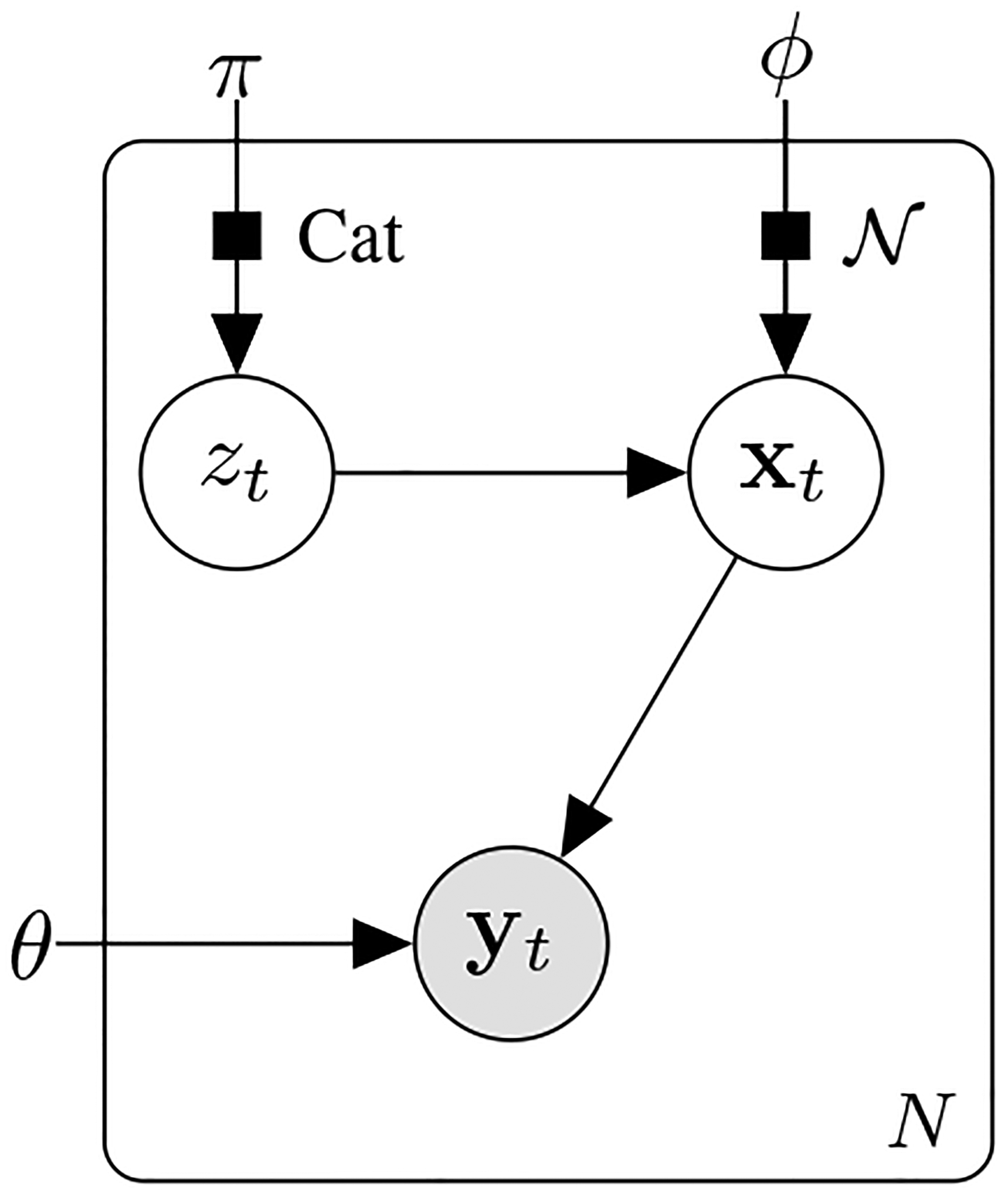
Graphical representation of the generative model.

B. The Inference

The matrix $\mathbf{Y}\in {\mathbb{R}}^{D\times T}$ will collectively denote all observed data so that its $t$-th column corresponds to the data point ${\mathbf{y}}_t$. Similarly, the matrix $\mathbf{F}\in {\mathbb{R}}^{D\times T}$ will denote the mapping latent variables, i.e., $f_{dt}=f_d\left({\mathbf{x}}_t\right)$ is associated with the observations ${\mathbf{y}}_t$. Analogously, $\mathbf{X}\in {\mathbb{R}}^{Q\times T},\mathbf{Z}\in \{1,\dots ,K{\}}^{K\times T}$ and $\mathbf{\Pi }\in [\mathrm{0,1}{]}^{K\times T}$ will store all low dimensional and intermediate latent variables. Further, we will refer to the rows of these matrices by the vectors ${\mathbf{y}}_d,{\mathbf{f}}_d,{\mathbf{x}}_q$, and ${\mathbf{z}}_k$. Given the latent variables, we assume independence over the data features, and given time, we assume independence over the latent dimensions. With these assumptions, we can write

$$p(\mathbf{Y},\mathbf{F},\mathbf{X},\mathbf{Z})=p(\mathbf{Y}\mid \mathbf{F})p(\mathbf{F}\mid \mathbf{X})p(\mathbf{X}\mid \mathbf{Z})P\left(\mathbf{Z}\right)$$ (18)

$$=\prod _{d=1}^{D}p\left({\mathbf{y}}_d\mid {\mathbf{f}}_d\right)p\left({\mathbf{f}}_d\mid \mathbf{X}\right)\prod _{q=1}^{Q}p\left({\mathbf{x}}_q\mid \mathbf{Z}\right)p\left(\mathbf{Z}∣\mathbf{\Pi }\right)\prod _{k=1}^{K}p\left({\pi }_k\mid \mathbf{t}\right).$$ (19)

We use a sparse spectrum approximation [16] of the Gaussian process introduced in the previous section. Common inference methods for Gaussian processes [12] become infeasible due to the non-differentiable sampling of the discrete variable $\mathbf{z}$. To optimize the latent variable $\mathbf{z}$, we therefore employ the Gumbel-Softmax relaxation technique. This method allows for differentiable sampling from a categorical distribution, enabling end-to-end training of the model using gradient-based optimization algorithms. The Gumbel-Softmax distribution approximates the categorical distribution by introducing noise from the Gumbel distribution and applying the softmax function to obtain a continuous relaxation.

V. Experiments and Results

A. Synthetic Data

We generate synthetic data using a Gaussian process framework, where the latent probabilities ${\tilde{\pi }}_{k,t}$ are drawn from a Gaussian process prior with mean zero and a covariance kernel $k\left(t,t^{\prime }\right)$. These latent probabilities are then normalized to obtain the probabilities ${\pi }_{k,t}$ [17]. The latent process $z_t$ is then sampled from a categorical distribution with parameter ${\pi }_t$, forming a discrete representation of the data. Subsequently, the latent processes $x_q\left(t\right)$ are generated from another Gaussian process with a covariance kernel composed of the temporal covariance $k\left(t,t^{\prime }\right)$ and $k\left(\pi ,{\pi }^{\prime }\right)$. Finally, the output ${\mathbf{y}}_{t+1}$ is obtained by applying a function $f_{\theta }$ to ${\mathbf{x}}_t$, with additive noise ${\mathit{ϵ}}_t$. In summary,

$${\tilde{\pi }}_k~𝒢𝒫\left(0,k\left(t,t^{\prime }\right)\right),$$ (20)

$${\pi }_k=\frac{\text{exp}\left({\tilde{\pi }}_{k,t}\right)}{\sum _{k^{\prime }=1}^K\text{exp}\left({\tilde{\pi }}_{k^{\prime },t}\right)},$$ (21)

$$z_t~p\left(z_t\mid {\mathit{\pi }}_t\right),{\mathit{\pi }}_t=\left[{\pi }_{1,t},\dots ,{\pi }_{K,t}\right],$$ (22)

$${\mathbf{x}}_q~𝒢𝒫\left(0,k\left(t,t^{\prime }\right)+k\left(\mathit{\pi },{\mathit{\pi }}^{\prime }\right)\right)$$ (23)

$${\mathbf{f}}_d~𝒢𝒫\left(0,k_f\left(\mathbf{x},{\mathbf{x}}^{\prime }\right)\right)$$ (24)

$$y_{dt}=f_d\left({\mathbf{x}}_t\right)+{ϵ}_{dt}.$$ (25)

The dimension of the categorical variable in this example is one, with $K=3$. The dimension of ${\mathbf{x}}_t$ is three ($Q=3$) and the number of observed time series ${\mathbf{y}}_t$ is 30 $(D=30)$. All kernels are RBF with different hyperparameters. We assumed we knew the onset of the categorical variable and attempted to predict the corresponding task, using only the inferred ${\stackrel{\mathbf{ˆ}}{\mathbf{z}}}_t$, to evaluate how much the model was able to compress the information in ${\stackrel{\mathbf{ˆ}}{\mathbf{z}}}_t$. The accuracy of the task prediction was 82.3%. It is clear that this discrete latent variable ${\stackrel{\mathbf{ˆ}}{\mathbf{z}}}_t$ was able to obtain the information about the task from the generated time series in a fully unsupervised fashion.

B. Real Data

To assess the effectiveness of our model on real data, we employed functional Magnetic Resonance Imaging (fMRI) data acquired from 35 individuals diagnosed with major depressive disorder. The dataset comprises multivariate time series extracted from Regions of Interest (ROIs) known to be implicated in depression.

The data were collected during the execution of diverse cognitive tasks, capturing subjects’ neural activity during both an anticipation phase (Anti) and a feedback phase (FB). The feedback stimuli presented images depicting expressions of happiness (Happy), neutrality (Neutral), or sadness (Sad) on the faces of familiar therapists.

In total, the dataset includes six distinct categorical variables and 375 ROIs. This comprehensive dataset enables a detailed exploration of neural dynamics in response to varied cognitive tasks and emotional stimuli, facilitating a robust assessment of our model’s performance in real-world scenarios. Figure 3 depicts how the read dataset looks like. We attempt to predict the underlying task using both latent processes $\mathbf{x}$ and the discrete latent process $\mathbf{z}$. The confusion matrices of these classifications are depicted in Fig. 4 (a) and (b). The dimensionality of $\mathbf{x}$ is 10, and the dimensionality of $z$ is one. We observe that the model successfully extracts information from the high-dimensional time series and summarizes them in $\mathbf{z}$ and $\mathbf{x}$. However, it’s worth noting that the accuracy using $\mathbf{z}$ alone will likely be lower, as the model is forced to compress the information into such a low dimension. Nevertheless, this low dimensionality is valuable for interpretability purposes. To further interpret the results, we selected one patient with high accuracy and plotted the probability of each task when $z=k$, for $k=1,\dots ,6$. Figure 5 illustrates these probabilities, demonstrating how the model has compressed the information about each task into the latent variable $\mathbf{z}$.”

Fig. 3:

Real Data: The dataset comprises 375 time series. Only five are visualized here.

Fig. 4:

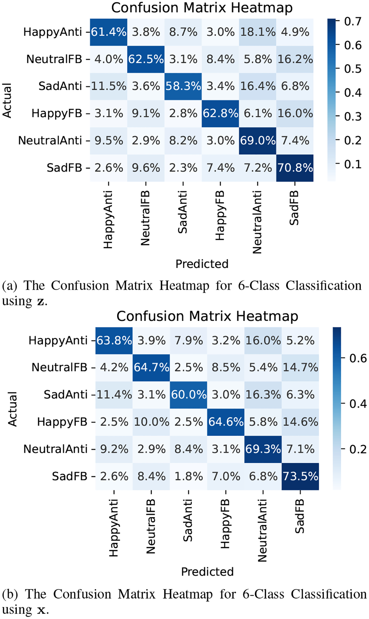
Downstream task using the learnt representation.

Fig. 5:

Task information embedded in $\mathbf{z}$ for a single selected patient.

VI. Conclusion

In this study, we introduced a novel deep architecture for interpretable representation learning in multivariate time series, particularly focusing on fMRI data analysis. Our approach effectively captures significant features while maintaining interpretability, as demonstrated through empirical assessments on synthetic and real-world fMRI data. By emphasizing the importance of interpretability and presenting the model’s efficacy, we contribute to advancing the field of discrete representation learning for complex time series. Future research can explore higher dimensional fMRI data as well as broader applications beyond fMRI analysis.

Fig. 2:

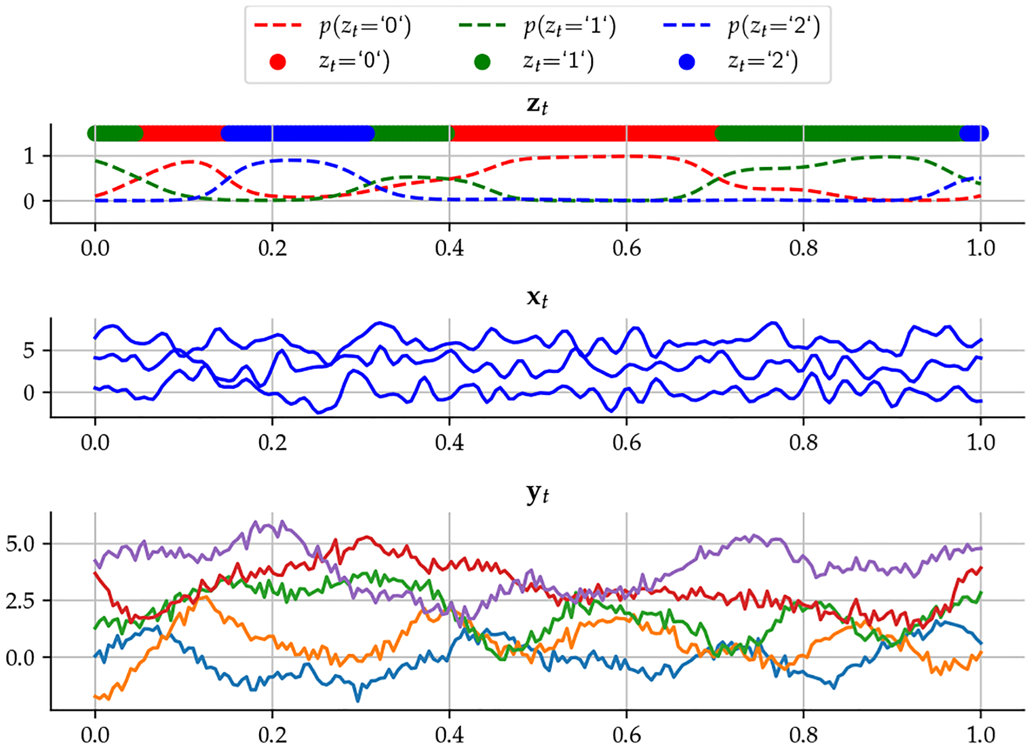
Synthetic data ${\mathbf{y}}_t$ and latent variables ${\mathbf{x}}_t$ and ${\mathbf{z}}_t$.

References

- [1].Ajirak Marzieh, Liu Yuhao, and Djurić Petar M, “Filtering of high-dimensional data for sequential classification,” in 27th International Conference on Information Fusion. IEEE, 2024. [Google Scholar]
- [2].Gal Yarin, Chen Yutian, and Ghahramani Zoubin, “Latent Gaussian processes for distribution estimation of multivariate categorical data,” in International Conference on Machine Learning, 2015, pp. 645–654. [Google Scholar]
- [3].Liu Yuhao, Ajirak Marzieh, and Djurić Petar M, “Sequential estimation of Gaussian process-based deep state-space models,” IEEE Transactions on Signal Processing, 2023. [Google Scholar]
- [4].Ajirak Marzieh and Djurić Petar M, “A Gaussian latent variable model for incomplete mixed type data,” in ICASSP 2023–2023 IEEE International Conference on Acoustics, Speech and Signal Processing (ICASSP). IEEE, 2023, pp. 1–5. [Google Scholar]
- [5].Ajirak Marzieh, Liu Yuhao, and Djurić Petar M, “Ensembles of Gaussian process latent variable models,” in 2022 European Signal Processing Conference (EUSIPCO), 2022. [Google Scholar]
- [6].Ajirak Marzieh, Heidi Preis, Lobel Marci, and Djurić Petar M, “Learning from heterogeneous data with deep Gaussian processes,” in International Workshop on Computational Advances in Multi-Sensor Adaptive Processing (CAMSAP). IEEE, 2023. [Google Scholar]
- [7].Maddison Chris J, Mnih Andriy, and Teh Yee Whye, “The concrete distribution: A continuous relaxation of discrete random variables,” arXiv preprint arXiv:1611.00712, 2016. [Google Scholar]
- [8].Jang Eric, Gu Shixiang, and Poole Ben, “Categorical reparameterization with gumbel-softmax,” arXiv preprint arXiv:1611.01144, 2016. [Google Scholar]
- [9].Mnih Andriy and Gregor Karol, “Neural variational inference and learning in belief networks,” in International Conference on Machine Learning. PMLR, 2014, pp. 1791–1799. [Google Scholar]
- [10].Mnih Andriy and Rezende Danilo J, “Variational inference for monte carlo objectives,” arXiv preprint arXiv:1602.06725, 2016. [Google Scholar]
- [11].Van Den Oord Aaron, Vinyals Oriol, et al. , “Neural discrete representation learning,” Advances in neural information processing systems, vol. 30, 2017. [Google Scholar]
- [12].Blei David M, Kucukelbir Alp, and McAuliffe Jon D, “Variational inference: A review for statisticians,” Journal of the American statistical Association, vol. 112, no. 518, pp. 859–877, 2017. [Google Scholar]
- [13].Rahimi Ali and Recht Benjamin, “Random features for large-scale kernel machines,” Advances in Neural Information Processing Systems, vol. 20, 2007. [Google Scholar]
- [14].Liu Yuhao, Ajirak Marzieh, and Djurić Petar M., “Sequential estimation of Gaussian process-based deep state-space models,” IEEE Transactions on Signal Processing, pp. 1–14, 2023. [Google Scholar]
- [15].Rasmussen Carl Edward, “Gaussian processes in machine learning,” in Summer School on Machine Learning. Springer, 2003, pp. 63–71. [Google Scholar]
- [16].Quiñonero-Candela Joaquin and Rasmussen Carl Edward, “A unifying view of sparse approximate gaussian process regression,” Journal of Machine Learning Research, vol. 6, no. Dec, pp. 1939–1959, 2005. [Google Scholar]
- [17].Damianou Andreas, Titsias Michalis, and Lawrence Neil, “Variational gaussian process dynamical systems,” Advances in neural information processing systems, vol. 24, 2011. [Google Scholar]