

Abstract
Although Chemical Transport Models (CTMs) such as the Community Multiscale Air Quality Model (CMAQ) have been used in linking observations of trace gases to emissions and developing vertical column distributions, there remain consistent biases between CTM simulations and satellite retrievals. Simulated tropospheric NO2 vertical column densities (VCDs) are generally higher over areas with large NO x sources when compared with retrievals, while an opposite bias is found over low NO x regions. Artificial (i.e., numerical) dilution in the model, where emissions are mathematically dispersed uniformly within the originating CTM grid, can impact modeled NO:NO2 ratios, while lower CTM VCD levels often observed over rural areas can be attributed to missing emission sources of NO x or flawed horizontal/vertical transport. Potential causes of both low and high biases are assessed in this study using CMAQ and Tropospheric Monitoring Instrument (TROPOMI) NO2 retrievals. It was found that more detailed modeling of NO x plumes to assess the NO:NO2 ratio in two power plant plumes can mitigate the effect of artificial computational dilution, reducing the bias and overall differences in the observed vs modeled plumes (errors reduced by 30%). Adjustments of upper tropospheric NO2 led to overall improvements, with a reduction in CMAQ bias (−43% to −29%) and improved spatial correlation (0.81 to 0.86). This study highlights the importance of having accurate modeled NO:NO2 ratios when comparing models to retrievals and the impact of unintentional numerical dilution.
Keywords: satellite retrievals, TROPOMI, NO2 vertical column densities, NO x ratio, power plants, chemical transport models


1. Introduction
Comparing satellite-derived nitrogen dioxide (NO2) fields with chemical transport model (CTM) results has proven to be a powerful approach in identifying potential errors in estimated nitrogen oxide (NO x = NO + NO2) emission inventories. − Before 2018, satellite-derived fields were relatively coarse (i.e., about 13 km or more). The new Tropospheric Monitoring Instrument (TROPOMI) has provided much finer resolution fields (approximately 4 km with oversampling on the order of 1 km) since then. These fields have been compared with similarly fine-scale regional CTMs such as the Community Multiscale Air Quality Model (CMAQ) to identify potential errors in emissions estimates. However, comparing modeled and TROPOMI NO2 vertical column densities (VCDs) to identify potential error sources in NO x emissions assumes that the modeled NO to NO2 ratio is correct. If the ratio is not accurate, there will be a mismatch between observed and CTM NO2 VCDs, even if the total modeled NO x in a column is accurate.
CTMs such as CMAQ are used when comparing modeled and observed VCDs because they can capture NO to NO2 conversion in the atmosphere and provide simulated vertical distributions of NO2 for calculating air mass factors (AMFs) used for diagnosing satellite retrievals. Studies have found that satellite observations and modeled VCDs show similar spatial distributions, supporting the use of satellite retrievals for assessing NO x emissions inventories.
However, in most of these high-resolution (i.e., ≤4 km) studies, CTM NO2 VCDs are higher than TROPOMI VCDs near large NO x emission sources (e.g., roadways, urban centers, power plants, and airports) with differences as high as 50–60%. − Some of these sources, such as power plants, have continuous emission monitoring systems (CEMs), common for electricity generating units (EGUs), such that the emissions from those sources are accurately known, and thus it may be assumed that errors in CTM NO x concentrations would be significantly minimized. This would suggest that such sources with CEMs can be used to assess potential biases in satellite retrievals with minimal error; however, the high model bias relative to satellite retrievals for these sources still exists.
One issue that impacts the retrieval comparison with Eulerian models such as CMAQ and GEOS-Chem when no plume-in-grid treatment is incorporated is the immediate dispersion (“well mixed”) of point source emissions within the computational grid cell of the source. The immediate dilution of NO x into the computational cell itself does not impact the total columnar abundance of NO x , but the overdilution allows the NO to react more rapidly with ozone (O3) to form NO2. This is because the artificial dilution increases the relative amount of ozone to NO x available for reaction, leading to more NO being oxidized to NO2 in CTMs. This numerical artifact would be most severe over computational grid sizes that are much larger than the plume width (e.g., >1 km horizontal spacing) so that much more NO is converted to NO2 in the model.
In the actual plume, plume NO2 concentrations are affected by chemical kinetics and thereby the relative initial concentrations of NO x and O3. Here, the large abundance of NO (which makes up 90–95% of fresh NO x emissions) will react to deplete the ozone in the plume such that near the source most of the plume NO x will continue to be found as NO since there is no more available ozone to react within the core of the plume. In this case, O3 serves as the limiting reagent, hindering further conversion of NO x to NO2.
The bias becomes larger when finer scale retrievals and model simulations are compared versus when using larger grids. This is because the modeled NO x levels along the plume are higher when using finer grids. Thus, while the advent of having fine scale (e.g., <5 km) NO2 fields from TROPOMI has led to being able to conduct more detailed and direct comparisons between satellite observations and modeled results, the smaller control volume actually exacerbates the problem of having a higher modeled NO2:NO ratio in the plume than actually occurs. , The well-mixed assumption near the source in smaller grids that have less diluted modeled NO2, in combination with artificial dilution of subgrid scale emissions over larger grids, results in higher modeled NO2 levels, with more NO x being simulated as NO2 instead of NO. This compounds the errors associated with differences in model resolution that influence the nonlinear chemistry of NO x . ,
A closely associated issue impacting the comparison of modeled vs observed NO2 VCDs is that most CTMs rapidly diffuse high pollutant concentrations horizontally and vertically , such that the plumes are quickly diffused not only in the single computational cell where they are emitted but also throughout the entire column that is within the mixed layer, which can be up to 1000 m thick. This also extends to horizontally adjacent grids, as well. Thus, the plume is computationally highly diluted almost immediately, and there is sufficient ozone to convert most of the emitted NO to NO2, further increasing the NO2 VCD differences between CTMs and retrievals.
In this study, the potential contribution from artificial dilution (vertical and horizontal diffusion of the plume) in CMAQ and differences from tropospheric TROPOMI NO2 VCD are assessed using a Gaussian plume model linked to a NO–NO2–O3 pseudosteady state (PSS) model. The focus here is on plumes from high NO x , elevated point sources, primarily EGUs. In high NO x plumes, the concentrations of oxidizing species such as O3 and OH will be reduced due to the high NO and low organic carbon levels. Also considered in this study is an adjustment to simulated NO2 in the upper troposphere to account for low model biases found in the upper troposphere, potentially due to a bias in the tropospheric/stratospheric exchange, underestimates of emission sources (i.e., aircraft cruise NO x or lightning emissions), or chemistry cycling of oxidized nitrogen species to NO x . Overall, we highlight the effect of these possible sources on the differences between the modeled and observed NO2 VCD.
We use TROPOMI retrievals because of their higher resolution and availability of more temporal data than previous satellite instruments such as the Ozone Monitoring Instrument (OMI) and the Global Ozone Monitoring Experiment (GOME), coupled with their superior performance. Using simulated vertical profiles from high resolution models also helps improve satellite retrievals. CMAQ was selected as the CTM due to its heavy reliance by U.S. regulatory agencies such as the Environmental Protection Agency (EPA) in assessing emissions changes and the effectiveness of environmental policies, its capabilities to simulate species concentrations at higher grid resolutions, and its wide use in past studies. We also use direct measurements of EGU emissions which reduces the amount of uncertainty in CTM results. Of note, the term CTM when used herein refers specifically to CMAQ simulated results.
2. Methods
2.1. CMAQ Simulations of VCDs and NO x Ratios
CTM results from Lawal et al., which compared NO2 VCDs derived from the Community Multiscale Air Quality (CMAQv5.3.2) chemical transport model with TROPOMI VCD retrievals over Atlanta, Georgia, were used. A detailed description of CMAQ and its governing chemical and physical processes can be found in Byun and Schere. Modeled NO2 VCDs near two power plants (Bowen and Scherer) whose NO x emissions are well characterized with CEMs were used to assess potential biases in TROPOMI. The WRF-SMOKE-CMAQ platform (Table S1) was used to simulate air quality over the 244 km × 244 km model domain (Figure ), with a horizontal grid spacing of 4 km and 32 vertical layers extending to ∼16 km (100 hPa) during the month of August of 2019. Anthropogenic emissions were from the National Emissions Inventory 2016v1 Emissions Modeling Platform and include a modified airport emissions inventory which integrates NEI ground based airport emissions with full-flight (i.e., cruise) emissions from the Aviation Emissions Inventory Code (AEICv2.1) emissions repository. , Lightning NO x emissions were calculated using a statistical parametrization method. Additionally, simulations with several EGUs (Figure S1), conducted in different parts of the U.S. for a wintertime (January 2016) and summertime period (July 2016) were included for additional analysis.
1.
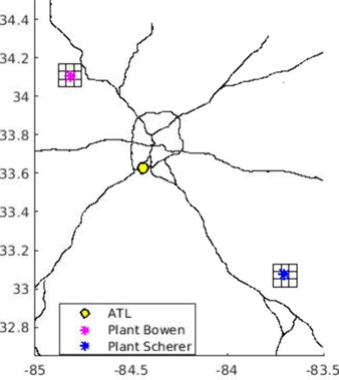
CMAQ modeling domain. Plant Bowen and Plant Scherer (both large electricity generation units) in northern Georgia (USA), with associated adjusted grids are shown, as are interstate highways. ATL is the Atlanta Hartsfield–Jackson International Airport.
2.2. TROPOMI NO2 Retrieval Process
TROPOMI follows a sun-synchronous orbit with an overpass time near 1:30 pm local solar time. The offline Level 2 v1.3 TROPOMI NO2 product developed by the Royal Netherlands Meteorological Institute (KNMI) accessed at NASA’s Goddard Earth Sciences Data and Information Services Center (GES DISC, https://tropomi.gesdisc.eosdis.nasa.gov/) was used in the study. Data are filtered to exclude pixels with solar zenith angles greater than 60°, quality flag (qa_value) less than 0.5, and cloud cover fraction (CLCF) criterion of less than 0.3, such that a total of 24 days out of the 31 days in August are used in this analysis. Seven of the 24 days had to be discarded due to missing data from pixels needed for analysis, resulting in a total of 17 days available for comparison of tropospheric TROPOMI and CMAQ NO2 VCDs. The level 2 (L2) product provides tropospheric VCDs, and the associated air mass factors (AMFs), which are calculated using vertical distributions from the TM5-MP model at 1° × 1°. In line with Cooper et al., , we used the provided averaging kernels and model vertical profiles from our higher resolution model to produce alternative AMFs which are then used to recalculate TROPOMI VCDs. For all CMAQ-TROPOMI tropospheric comparisons, TROPOMI L2 data were remapped to the CMAQ grid using oversampling.
2.3. Gaussian Plume and Pseudosteady State Modeling (Gaussian-PSS)
The potential level of a CTM overestimating the conversion of NO to NO2 in an EGU plume was first evaluated by simulating plume growth using a Gaussian plume model of a NO x containing plume into an atmosphere with pre-existing ozone levels, assuming a pseudosteady state balance (Gaussian-PSS) between O3, NO, and NO2. First, the NO x concentrations in the plume are calculated using eq where x, y, and z are the downwind, crosswind, and vertical locations relative to the effective emission location.
| 1 |
Q is the source strength, U is the wind speed, and σ y and σ z are the horizontal and vertical diffusivities which are functions of x. Of note, the stability class and equations used to calculate σ y and σ z , as referenced from Seinfeld and Pandis can be found in the accompanying Supporting Information (SI). This equation assumes that NO x is conserved, recognizing that oxidation of NO x to nitric acid and other photochemical species will occur relatively slowly in the plume. Of note, our analysis follows the plumes for about 2 h. Next, the NO x concentrations are used in a pseudosteady state model (eqs -), to calculate the distribution of NO, NO2, and O3 where [NO]0, [NO2]0, and [O3]0 are the initial levels of those species (i.e., levels that would occur without chemical conversion).
| 2 |
| 3 |
| 4 |
Here j NO 2 is the photolysis rate of NO2, and k O3+NO is the rate of reaction between NO and O3 to form NO2 and oxygen. In our case, we assume that the initial NO and NO2 concentrations are [NO]0 = 0.9*[NO x ]0 and [NO2]0 = 0.1*[NO x ]0, respectively, using measured ratios from a previous study and where [NO x ] represents the total NO x concentrations resulting from the EGU emissions. The resulting concentration distributions can be integrated numerically over the three-dimensional domain to find the fraction of the NO x in the plume, that is NO.
As a test case, the NO:NO2 ratio in a plume was calculated as a function of distance using the above approach for an elevated plume using a slightly unstable atmosphere. We use the American Society of Mechanical Engineers (ASME) relationships between the dispersion coefficients as a function of x, a NO x source strength of Q = 50 × 103 kg/day (∼50 tons/day: a moderately sized power plant with emission controls), and a wind velocity of 5 m s–1 to obtain [NO x ] from eq . To calculate the pseudosteady state ozone distribution (eq ), we used a 1:30 pm approximate local time of the TROPOMI overpass in the southeastern US, leading to a j NO 2 value of 0.009 s–1 and an O3 + NO reaction rate constant (k O3+NO) of 2 × 10–14 cm3 mol–1 s–1. We set the initial ozone concentration [O3]0 to 60 ppb, similar to what might be expected on a summer day in the Southeast. The resulting concentration fields were then integrated over the plume from its origin downwind for horizontal distances in the x and y directions, between 1 and 10 km and up to 8 km in the vertical direction (z) to calculate the fraction of NO x that is NO and NO2 (eq and eq ) in the plume. Of note, a similar analysis can be done for concentrated ground level sources, including highways (using a line-source model) and for larger areas with high levels of NO x emissions (e.g., the urban cores of cities, airports, and rail yards). Such an analysis and application is more complicated as urban areas have a mix of source and source strengths and will be subject to different NO x chemistry than might be observed in a plume from an EGU. Further, highways are not isolated, and downwind transport of NO x from upstream sources is important. This is discussed in further detail in the SI.
Elshout et al. suggested that a combination of mixing and kinetics dynamics govern NO oxidation; however, Janssen et al. proposed that within a plume this process is largely kinetically driven. To this end, we use our Gaussian-PSS model to test these dynamics with three scenarios, one where the O3 levels are kept at 60 ppb and U is 5 m/s, a scenario where we lower ozone to 10 ppb, keeping U at 5 m/s, and the last, where O3 levels are kept at 60 ppb but wind speed is increased to 10 m/s. The results are in the Supporting Information and are discussed in the Results section.
Lastly, we demonstrate, using the Gaussian-PSS model, how chemical mischaracterization resulting from numerical dilution due to the Eulerian grid size of the CTM changes the distribution of modeled NO x between NO2 and NO in the originating grid of a power plant plume.
2.4. Adjustment of NO2 in Upper-Tropospheric CTM Levels
Modeled rural NO2 from CTMs tends to be biased low when compared with aircraft and satellite-based observations, a trend that is consistent across studies despite differences in season, climate, and regions. These differences are also observed with other Eulerian based CTMs as well, such as GEOS-CHEM. These CTM biases could result from errors in atmospheric mixing, atmospheric reactions, and emission inventories. For example, potential errors related to tropospheric/stratospheric exchange, rapid chemical depletion in the model or an emissions bias (e.g., from aircraft or lightning), and other background sources such as chemical pathways converting oxidized nitrogen species to NO x could account for the biases. Mischaracterization of NO x from lightning which is particularly important for the month of August and aircraft emissions can account for a 30% to 40% increase in upper tropospheric NO x . Given the range of potential reasons why upper level NO2 levels may be biased low, adjustments of modeled simulated upper tropospheric NO2 (i.e., see Figures S2 and S3) are done as a sensitivity study here. Observations of upper tropospheric NO2between 450 hPa and 180 hPausing cloud slicing suggest that NO2 concentrations are usually between 50 and 100 ppt in the Southeastern United States during summertime (Marais et al.), though recent analyses suggest prior estimates of upper tropospheric NO2 might be higher (Shah et al.). In our baseline CTM simulation, we find that the average simulated NO2 concentrations in the upper troposphere are 30–40 ppt (Table S2). Thus, as a sensitivity study to determine the potential impact of errors from underestimated NO2 and missing emission sources, we recalculate the simulated upper tropospheric NO2 concentrations while keeping the simulated NO x mass balance from the CMAQ base case constant at elevations above 8 km from ∼40 to ∼80 ppt. As a result, this adjustment falls more in line with Marais et al.’s observations of NO2 (i.e., ∼100 pt) within the uncertainty of the measurements.
2.5. Sensitivity Assessments for Modeled Domain
We evaluated how changes in the modeled NO:NO2 ratios of two power plant plumes and their adjacent grids (Figure ), and upper tropospheric NO x ratios at altitudes above ∼8 km, impacted the comparison with TROPOMI VCDs. Adjustments are first made to power plant plumes (up to ∼8 km) by using the estimated Gaussian plume calculations described in Section . NO x ratio adjustments in the upper troposphere as described in Section are then incorporated. New AMFs are calculated using the adjusted vertical NO2 profile studies. , The effect of adjusted AMFs on NO2 VCDs between each CTM adjusted case and TROPOMI VCDs is evaluated using several statistical metrics such as the root-mean-square error (RMSE) and normalized mean bias (NMB). Temporal and spatial averaging of TROPOMI VCDs reduces the random component of the uncertainty associated with TROPOMI AMFs, and focus on difference metrics such as bias and RMSE minimizes the systematic component of error in this analysis. ,
3. Results and Discussion
3.1. NO x Ratio EGU Gaussian Plume Calculations vs CMAQ EGU NO x Distributions
For the first 2 km of a plume (corresponding to a grid size of 4 km, assuming that, on average, the source is in the middle of the grid), approximately 90% of the NO x will be in the form of NO (Figure S4). Results from the Gaussian–PSS model show that in each consecutive grid the fraction that is NO decreases as NO is oxidized to NO2 (Figure a). In contrast, in CMAQ, this conversion to NO2 happens rapidly within the same computational grid as that of the EGU plume source. The CMAQ-modeled NO x ratio in the grid cell containing Plant Scherer (and similarly Plant Bowen) shows an ∼0.27/0.73 split between NO and NO2 (Figure b). Overall, it takes up to nearly 8 grid cells (∼30 km) from the source grid before the NO x ratios in the Gaussian model approach those modeled by the CTM. When the vertical profiles of NO and NO2 ratios are plotted, relatively little vertical variation in the ratio is seen (Figure S5).
2.

Fraction of the total NO x that is NO and NO2 plotted at various distances from the plume source. a) NO and NO2 ratios calculated using the Gaussian plume and PSS approximation model. b) NO and NO2 ratios near Plant Scherer (Figure ) as calculated from the CMAQ simulations.
While there are limits to the plume dynamics calculations in the Gaussian–PSS model (e.g., the interaction with both the ground and top of the boundary layer, radial wind shifts), these results provide a more realistic representation of the actual NO x ratios expected in a plume and are comparable to the findings in other similar modeling studies. In Melo et al., for example, modeled results of exiting concentrations of a power plant plume found 49% of total NO x to be NO2 at distances up to 40 km, matching measurements. Additionally, measurements of the fraction of NO x as NO2 in plumes (up to ∼2.7 km) were no larger than 0.17. In Janssen et al., measured NO:NO2 ratios were mostly below 0.5 at distances up to 10 km, only increasing at those distances if higher ozone mixing ratios and wind speeds (i.e., dilution) were observed. The results here can also be compared to other independent observations that show the core of a power plant plume at 11 km and 36 km downwind having greatly reduced ozone due to depletion through reaction with NO and in accord with the observations of NO:NO2 ratios in power plant plumes, lending further support to the calculated plume NO x ratios presented here. Also, 2019 measurements of a plume from Plant Scherer found near equal levels of NO and NO2 within 20 km, supporting calculations in Figure a.
Lastly, while the potential for the rapid numerical vertical dilution of NO x to lead to high NO:NO2 ratios in CTM simulations is not fully quantified here, these results show that it readily explains much of the potential differences in the NO2 VCD comparisons. More detailed quantification could be addressed by using in situ measurements from airborne campaigns that acquire data within plumes, as well as high spatial resolution (i.e., 250 m) NO2 column density information from airborne spectrometers like the GEO-CAPE Airborne Simulator (GCAS). Further, conducting dispersion model calculations (e.g., using AERMOD) for the urban area and comparing NO:NO2 ratios calculated using the Gaussian–PSS or more detailed large eddy simulations can be insightful.
We note that the artificially high rate of NO oxidation to NO2 within the plumes as a result of numerical dilution is not limited to those EGUs but can be seen for other EGUs within the CONUS modeling domain, located in different regions across the U.S. Figure S6 shows similarly modeled NO x ratios for the Navajo Generating Station in Arizona and Plant Mountaineer, located in West Virginia. This is also observed during winter and summer months as well. A similar emission profile of NO and NO2 is shown with Plant Mountaineer and Plant Bowen in Figure S7.
3.2. Plume Dynamics in CMAQ and Gaussian–PSS Models
The physical and chemical processes in plumes such as those originating from power plants differ from ambient (regional) air chemistry and processes, and concentrations of NO, NO2 and O3, and OH will be different from the magnitudes discussed in Valin et al., where the focus was on urban plumes. As noted in Elshout et al., NO oxidation of power plant plumes is strongly dependent upon mixing, and under ambient conditions, high oxidation rates of NO due to ozone entrainment near the plume edges are likely to be observed. In the center of the plume, it is more likely that the level of the O3 will be low due to depletion from high NO concentrations, so less oxidation will occur. We model the relationship between turbulent mixing and oxidant ratios with the Gaussian–PSS model by comparing the three scenarios discussed in the methods in Section . Results presented in Figure S8 show that when O3 is set at 60 ppb NO oxidations to NO2 under two wind speeds (Figure S9(a), U = 5 m/s, and Figure S7(c), U = 10 m/s) are similar. When the levels of O3 are reduced to 10 ppb (Figure S8(b)), NO oxidation is considerably reduced, and a large proportion of NO x remains largely as NO near the source. This has important consequences when using satellite observations to help identify and quantify the emissions from large NO x sources, including power plants and airports because on days with low ozone only a small fraction of the NO will be converted to NO2, and the model bias in the NO2 to NO x ratio can be higher on low ozone days. Similarly, on days when the atmosphere is more stable, the plume would remain more concentrated near the source, leading to less of a NO-to-NO2 transformation.
3.3. Impact of Numerical Dilution and Diffusion
The Gaussian–PSS model described in Section is used to model NO x within the originating grid of a power plant plume to illustrate how chemical mischaracterization resulting from numerical dilution due to the Eulerian grid size of the CTM changes the distribution of modeled NO x between NO2 and NO. The results of this case study with the Gaussian plume model are presented in Figure . Changes in NO x distribution for different CTM grid dimensions of x and y (i.e., Figure a) are plotted for three different emission rates of NO x . Initially, NO/NO2 ratios are similar, irrespective of the emission rates at smaller grid sizes (Figure b), but then the results show an increasing conversion of NO to NO2 as grid size changes. In all cases, an increase in NO x conversion to NO2 is seen as grid size increases irrespective of emissions flux in the concentrated NO x plume. Further detailed discussion about the model applications can be found in the SI.
3.

a) Changes in model grid volume as dimensions in x and y are adjusted. b) Shows for three different emission rates how NO2 increases steadily as the grid sizes are adjusted to what is shown in (a).
3.4. NO:NO2 Ratio Adjustments on Simulated CMAQ NO2 VCDs of Power Plants
In the recent comparison of TROPOMI-derived NO2 VCDs and CMAQ simulations conducted using a 4 km grid resolution in the Atlanta, Georgia, USA, area, the TROPOMI-derived NO2 VCDs were about 50% of those derived using CMAQ (Figure a). In Goldberg et al., a similar disagreement between TROPOMI and a CTM was found near the Martin Lake, TX, power plant, though they posit that modeling parameters (i.e., NO2 chemical and dispersion lifetime) in combination with model resolution are a potential source of the discrepancy. Here, we attempt to correct for the rapid numerical dilution effect on NO to NO2 oxidation as if the numerical control volume was representative of the actual process, by imposing the 2/3 NO/NO x ratio as observed near the source in Janssen et al. in the boundary layer in the vertical column directly above the power plant and 1/2 in the vertical columns of the eight grids adjacent to the grid with the power plant. This is done with the understanding that emissions from EGU plumes primarily dominate NO x within the boundary layer of the column directly above the EGU. Based on reaction kinetics and experimental measurements, total NO x would largely exist as NO near the source. Further, gaseous oxidants such as O3 are rapidly depleted in such a plume, due to high NO concentration, thus limiting further conversion of NO to NO2. The eight adjacent grids were selected because for the most part the simulated plumes around each power plant appeared to persist only for those adjacent grids, dissipating to a steady profile beyond the 8 km radius around each plant with most experimental models showing at best a steady NO2/NO x ratio of 0.5 to 0.6 downwind of the source. , A similar idea involves averaging NO x around point sources horizontally rather than vertically to preserve the strong NO x gradients observed and constrain the NO x ratios. In this case, it was found, after recalculation of the AMFs, that the RMSE at both sites is decreased on average by 30% (Figure b and Table S3; Bowen: 2.0 to 1.4 × 10¹⁵ molecules/cm2; Scherer: 1.8 to 1.2 × 10¹⁵ molecules/cm2).
4.

a–c) TROPOMI NO2 VCD plots. d–f) CMAQ-TROPOMI NO2 VCD difference plots. g–i) Respective density scatter plots from scenarios in figures d to f. (a,d,g) Represent the base case with no adjustments for potential NO:NO2 model differences in NO x elevated plumes at two EGUs (Plant Bowen and Plant Scherer) and in the upper troposphere. (b,e,h) Show adjustments of NO x bias in elevated plumes at the two EGUs. (c,f,i) Show adjustments of NO x bias in elevated plumes at both EGUs and at higher altitudes above 8 km. Black lines are Interstate highways. The red and black dots in (g–i) represent the EGUs and the surrounding 8 grid cells as depicted in Figure . Data from the plots are averaged over the 17 selected days in August 2019.
There is further evidence that artificial dilution could be a large source of the discrepancies between CTM calculated NO2 VCDs and TROPOMI (or other satellite-based products) near large NO x sources when looking at spatial biases between the two. For instance, the degree of difference between the two diminishes downwind from the source fairly quickly for both the power plants and over the city (Figure d and e). If the NO x mass flux was constantly biased high or low in the model simulations, a persistent bias downwind of the sources would be found as most of the NO would be converted to NO2. Looking specifically at the two power plants from the initial base case, the highest differences were found just over the sources and rapidly dissipated downwind. Further, at one of the largest and more dispersed NO x sources in the model region, the Atlanta airport (Figure ), there is a large positive difference right over the airport itself, but that also goes away within one or two surrounding adjacent grid cells. Over such small distances (i.e., 2, 3, or 4 km grid cells), a little of the NO x would have been converted to nitric acid, suggesting not only that the modeled mass emissions of NO x are approximately correct and conserved but also that at distances further away where most of the NO x is NO2 (i.e., observed negative bias) even lower modeled NO2 is observed. This lends further credence to the hypothesis that CTMs overestimate the NO to NO2 conversion very near the source, an effect of artificial dilution. The model also has lower than observed NO:NO2 ratios when compared to ground observations in high source regions, also suggesting more rapid NO to NO2 oxidation (Figures S9 and S10).
3.5. Impact of Upper Troposphere NO2 Adjustments
Differences in modeled and TROPOMI VCDs extend beyond areas near highly emitting NO x sources. Modeled NO2 VCDs tend to be lower than those of satellite-based observations (Figure ). This could be partly due to an underestimate in background NO2, which could include an underestimate of stratospheric NO y transport or an underestimate of biogenic/geogenic NO x emissions, both which have an increasing contribution to total NO x as anthropogenic NO x emissions are reduced. A follow up study indicated that inventory inputs to CTMs were likely missing a significant portion of nonanthropogenic background emissions that could contribute to more NO2 partitioning. For example, additional (i.e., beyond that included in the current modeling) lightning-induced NO x could account for some unaccounted for NO2. , Regional CTM emission inventories that do not include cruise emissions could also lead to underestimates of NO2 in the upper troposphere as well. , Both can help explain why modeled NO2 VCDs in more rural areas are lower than the observations.
Here, in addition to the EGU plume adjustments, we increased the average upper tropospheric NO2 above 8 km from ∼30 ppt (Figure S2) to ∼80 ppt (Figure S3) to be more in line with Marais et al. This level of adjustment is also in line with Shah et al.’s findings of 1 × 10¹⁴ molecules/cm2 uncertainty with model simulations. When this modification is made, the RMSE is reduced from 1.12 to 0.70 × 10¹⁵ molecules/cm2. In Figure i, the overall NMB is reduced from −43% to −29% (Table ). The grids where a high bias in CMAQ remains are near the Atlanta airport and downwind of the urban core.
1. Tabulated Performance Metrics of NO2 Vertical Column Densities of CMAQ and TROPOMI .
| Adjustments | Data cut off | NMB % | Absolute bias 1015 molecules/cm2 | Mean CMAQ 1015 molecules/cm2 | Mean TROPOMI 1015 molecules/cm2 | Slope | Pearson correlation | RMSE 1015 molecules/cm2 | No. of data points |
|---|---|---|---|---|---|---|---|---|---|
| CMAQInitial | All Data | –43 | –1.04 | 1.4 | 2.5 | 0.76 | 0.81 | 1.12 | 2665 |
| <4.5 | –44 | –1.05 | 1.4 | 2.5 | 0.88 | 0.82 | 1.25 | 2644 | |
| ≥4.5 | 22 | 0.93 | 5.5 | 4.6 | 0.17 | 0.29 | 2.63 | 21 | |
| EGU plume adjustments | All Data | –43.6 | –1.0 | 1.4 | 2.5 | 0.82 | 0.82 | 1.1 | 2665 |
| <4.5 | –43.9 | –1.1 | 1.4 | 2.5 | 0.87 | 0.82 | 1.2 | 2649 | |
| ≥4.5 | 10.4 | 0.45 | 5.2 | 4.8 | 0.53 | 0.57 | 0.70 | 16 | |
| Upper Tropospheric adjustments (>8 km) | All Data | –28.5 | –0.61 | 1.6 | 2.2 | 0.79 | 0.85 | 0.72 | 2665 |
| <4.5 | –29.0 | –0.62 | 1.6 | 2.2 | 0.92 | 0.86 | 0.50 | 2639 | |
| ≥4.5 | 28.2 | 1.12 | 5.5 | 4.3 | 0.16 | 0.27 | 2.92 | 26 | |
| EGU and Upper Tropospheric (>8 km) adjustments | All Data | –29 | –0.61 | 1.6 | 2.2 | 0.85 | 0.86 | 0.70 | 2665 |
| <4.5 | –29 | –0.62 | 1.6 | 2.2 | 0.91 | 0.86 | 0.49 | 2644 | |
| ≥4.5 | 17 | 0.70 | 5.3 | 4.5 | 0.54 | 0.57 | 0.98 | 21 |
Results were tabulated using the represented number of grid points (Figure ) for the 17 selected simulation days and are separated into three categories: all NO2 VCD data points, NO2 VCDs less than 4.5 × 10¹⁵ molecules/cm2, and NO2 VCDs greater than 4.5 × 10¹⁵ molecules/cm2.
3.6. AMF Differences
Lastly, we look at the changes in AMF from the adjustments made in this study. Here we compare the results from the base case with the combined EGU NO x ratio adjustment and the upper-tropospheric NO2 adjustments. Distributions of AMFs from the base (initial) case and the recalculated AMFs from the adjustments (Figures S11 and S12, respectively) show that the adjustment led to a slight increase in average AMFs (i.e., 0.88 to 1.0). This 15% increase in the AMF, albeit small, led to a substantial decrease in overall NMB (Table ) and a greater spread over the 1–1 line (Figure i). The effect of this change was even more notable than the differences in CMAQ results between the base CMAQ case (i.e., 3D Base Case) and a default inventory (Table S4).
3.7. Limitations
This study is limited in its analysis to one satellite instrument and one computational Eulerian model. While variability in results might occur from different mixing regimes, inputs and chemical mechanisms among different models, the numerical dilution effect is common to Eulerian models when subgrid scale emissions are simulated ,, and this artifact is likely to be observed in other Eulerian models without a Plume-in-Grid treatment. , Another concern is the short time span used in this analysis (i.e., August 2019) and whether the results would be impacted if a longer time frame was used. As this study directly builds upon the findings of the previous study, it was necessary to use the same time frame in our assessment. It is also worth noting that the numerical effect of artificial dilution in CTMs is not affected by the choice of the season, region, or time span (see discussion in the SI). Simulations of multiple EGUs conducted at different times (i.e., 2016 vs 2019, summer vs winter) support the generality of the findings. Future work should consider the incorporation of a Plume-in-Grid model in an Eulerian model and evaluation of these effects at distances that extend beyond plume origins. With the availability of future satellite products at higher resolution than TROPOMI, such as TEMPO, additional analysis done at higher resolutions of CTMs will be insightful.
Lastly, while this paper focuses mainly on modeled NO2, it is likely that there will also be some impact on OH and O3, both of which react with NO x , although the extent is not specifically addressed or quantified here. However, a change in the NO2 could lead to changes in the modeled O3 in the power plant plume. Another effect, primarily near the source, is that modeled NO2 will be more widely dispersed, leading to higher O3 and OH levels, increasing HNO3 formation and aerosol nitrate.
3.8. Implications
The comparison of modeled and satellite observed NO2 VCDs highlights the importance of accounting for differences in modeled NO:NO2 ratios that stem from artificial plume dilution near large stack emissions. For instance, the change in normalized mean bias (NMB) as shown in Table (NMB: 22% to 10.4%) suggests that the seemingly large difference between TROPOMI and CTM VCDs over high emitting NO x sources could be partially due to overly rapid NO to NO2 conversion in the model. Not accounting for the effect of artificial dilution can result in modeled NO2 VCD bias, where increases in the NO2:NO x from 0.5 to as high as 0.8 were seen under highly convective conditions. Missing NO x emissions could degrade the comparison as well.
One approach to adjust for differences occurring from numerical diffusion in CTMs is to use a Plume-in-Grid model within the CTM to account for rapid dispersion effects over the computational grid; however, there are still limitations with those solutions, one being the computational requirements for finer-scaled applications. It is also important to consider similar treatment for other ground-based high-NO x emitting sources besides EGUs. For instance, NO x emissions from sources such as airports, where landing and takeoff emissions are spatially categorized as ground level emissions in regulatory models, should more realistically be treated as elevated-plume sources as well. ,− Further, to address potential errors in modeled upper troposphere mixing ratios, given the uncertainty in the NO:NO2 estimates, postsimulation recomputation of CTM-calculated VCDs can be employed as was done here. However, using observed measurements when available may introduce uncertainty. Of further note, to address the potential bias in the CTM-modeled NO2 VCDs over nonpoint sources with high levels of surface emissions, further analysis is recommended (e.g., using a model with a detailed ground-level dispersion approach or using observations if available).
While this paper focuses mainly on how rapid artificial model dilution impacts the NO:NO2 ratio and the resulting comparison between modeled and observed VCDs, the rapid dilution would also impact local OH, O3, and nitrate levels. The relative impact of mischaracterized physical processes such as convective transport and missing emission sources was also assessed in this study. Findings show that emission sources and oxidant chemistry could reduce model biases in the upper troposphere and rural areas.
This analysis shows that unless the columnar NO:NO2 ratio is captured by the model using fine-scale model calculations to compare with VCD observations, developing a top-down emissions inventory could result in erroneous estimates for strong NO x sources. These results also provide further support that CTM simulations of NO2 in the upper troposphere are biased low. Further analysis of how uncertainties in the modeled NO2 impact using satellite NO2 observations for emissions inventory assessment and top-down inventory development is an important area for future research.
Supplementary Material
Acknowledgments
The authors are grateful for the funding support of the National Science Foundation under grants 1444745–SRN: Integrated urban infrastructure solutions for environmentally sustainable, healthy, and livable cities, and EEC-2127509: The American Society for Engineering Education (ASEE). We also want to thank NASA’s Health and Air Quality Applied Sciences Team (HAQAST) program (Grant #80NSSC21K0506). We acknowledge past and current members of the NSF SRN and NASA HAQAST teams for their support on this project. The contents of this paper are solely the responsibility of the grantee and do not necessarily represent the official views of the supporting agencies. Further, the US government does not endorse the purchase of any commercial products or services mentioned in the publication.
The Supporting Information is available free of charge at https://pubs.acs.org/doi/10.1021/acsestair.4c00198.
Additional details on methods, equations, materials; a map of EGU NO x emissions, including plotted vertical profiles of simulated NO x ratios from CMAQ, tabulated simulated NOx, tabulated results of TROPOMI, and CMAQ NO2 vertical column densities; and additional figures showing CMAQ and TROPOMI VCDs and recalculated AMFs (PDF)
b.
U.S. Environmental Protection Agency, Research Triangle Park, NC 27709, USA
The manuscript was reviewed by all authors. All authors have given approval to the final version of the manuscript. Abiola S. Lawal: Methods, Software, Validation, Formal analysis, Investigation, Data curation, Writing – review and editing, Visualization. T. Nash Skipper: Methods, Software, Validation, Formal analysis, Investigation, Data curation, Writing – review and editing. Cesunica E. Ivey: Methods, Validation, Formal analysis, Resources, Writing – review and editing, Supervision, Funding acquisition. Daniel L. Goldberg: Methods, Validation, Formal analysis, Resources, Writing – review and editing. Jennifer Kaiser: Methods, Software, Validation, Formal analysis, Investigation, Data curation, Resources, Writing – review and editing, Visualization, Supervision, Project administration, Funding acquisition. Armistead G. Russell: Conceptualization, Methods, Validation, Formal analysis, Investigation, Resources, Writing – original draft, review and editing, Visualization, Supervision, Project administration, Funding acquisition.
The authors declare no competing financial interest.
References
- Ialongo I., Virta H., Eskes H., Hovila J., Douros J.. Comparison of TROPOMI/Sentinel-5 Precursor NO2 observations with ground-based measurements in Helsinki. Atmospheric Measurement Techniques. 2020;13(1):205–218. doi: 10.5194/amt-13-205-2020. [DOI] [Google Scholar]
- Lorente A., Boersma K. F., Eskes H. J., Veefkind J. P., van Geffen J. H. G. M., de Zeeuw M. B., Denier van der Gon H. A. C., Beirle S., Krol M. C.. Quantification of nitrogen oxides emissions from build-up of pollution over Paris with TROPOMI. Sci. Rep. 2019;9(1):20033. doi: 10.1038/s41598-019-56428-5. [DOI] [PMC free article] [PubMed] [Google Scholar]
- Kim H. C., Kim S., Lee S.-H., Kim B.-U., Lee P.. Fine-Scale Columnar and Surface NOx Concentrations over South Korea: Comparison of Surface Monitors, TROPOMI, CMAQ and CAPSS Inventory. Atmosphere. 2020;11(1):101. doi: 10.3390/atmos11010101. [DOI] [Google Scholar]
- Kim S.-W., Heckel A., Frost G. J., Richter A., Gleason J., Burrows J. P., McKeen S., Hsie E.-Y., Granier C., Trainer M.. NO2 columns in the western United States observed from space and simulated by a regional chemistry model and their implications for NOx emissions. J. Geophys. Res. 2009 doi: 10.1029/2008JD011343. [DOI] [Google Scholar]
- Copernicus Space Component Mission Management Team. S5P Products. https://sentinels.copernicus.eu/web/sentinel/data-products/-/asset_publisher/fp37fc19FN8F/content/sentinel-5-precursor-level-2-nitrogen-dioxide (accessed 2021 Aug 2).
- Binkowski F. S., Roselle S. J.. Models-3 Community Multiscale Air Quality (CMAQ) model aerosol component 1. Model description. Journal of Geophysical Research: Atmospheres. 2003 doi: 10.1029/2001JD001409. [DOI] [Google Scholar]
- Angle R. P., Sandhu H. S., Schnitzler W. J.. Observed and Predicted Values of N02/NOx in the Exhaust Plume from a Compressor Installation. Journal of the Air Pollution Control Association. 1979;29(3):253–255. doi: 10.1080/00022470.1979.10470789. [DOI] [Google Scholar]
- Palmer P. I., Jacob D. J., Chance K., Martin R. V., Spurr R. J. D., Kurosu T. P., Bey I., Yantosca R., Fiore A., Li Q.. Air mass factor formulation for spectroscopic measurements from satellites: Application to formaldehyde retrievals from the Global Ozone Monitoring Experiment. Journal of Geophysical Research: Atmospheres. 2001;106(D13):14539–14550. doi: 10.1029/2000JD900772. [DOI] [Google Scholar]
- Kim H. C., Kim S., Lee S.-H., Kim B.-U., Lee P.. Fine-Scale Columnar and Surface NOx Concentrations over South Korea: Comparison of Surface Monitors, TROPOMI, CMAQ and CAPSS Inventory. Atmosphere. 2020;11(1):101. doi: 10.3390/atmos11010101. [DOI] [Google Scholar]
- Jeong U., Hong H.. Assessment of Tropospheric Concentrations of NO2 from the TROPOMI/Sentinel-5 Precursor for the Estimation of Long-Term Exposure to Surface NO2 over South Korea. Remote Sensing. 2021;13(10):1877. doi: 10.3390/rs13101877. [DOI] [Google Scholar]
- Verhoelst T., Compernolle S., Pinardi G., Lambert J. C., Eskes H. J., Eichmann K. U., Fjæraa A. M., Granville J., Niemeijer S., Cede A.. et al. Ground-based validation of the Copernicus Sentinel-5P TROPOMI NO2 measurements with the NDACC ZSL-DOAS, MAX-DOAS and Pandonia global networks. Atmos. Meas. Technol. 2021;14(1):481–510. doi: 10.5194/amt-14-481-2021. [DOI] [Google Scholar]
- Liu S., Valks P., Pinardi G., Xu J., Chan K. L., Argyrouli A., Lutz R., Beirle S., Khorsandi E., Baier F.. et al. An improved TROPOMI tropospheric NO2 research product over Europe. Atmos. Meas. Technol. 2021;14(11):7297–7327. doi: 10.5194/amt-14-7297-2021. [DOI] [Google Scholar]
- Li M., McDonald B. C., McKeen S. A., Eskes H., Levelt P., Francoeur C., Harkins C., He J., Barth M., Henze D. K.. Assessment of Updated Fuel-Based Emissions Inventories Over the Contiguous United States Using TROPOMI NO2 Retrievals. Journal of Geophysical Research: Atmospheres. 2021 doi: 10.1029/2021JD035484. [DOI] [Google Scholar]
- Goldberg D. L., Lu Z., Streets D. G., de Foy B., Griffin D., McLinden C. A., Lamsal L. N., Krotkov N. A., Eskes H.. Enhanced Capabilities of TROPOMI NO2: Estimating NOX from North American Cities and Power Plants. Environ. Sci. Technol. 2019;53(21):12594–12601. doi: 10.1021/acs.est.9b04488. [DOI] [PubMed] [Google Scholar]
- Byun D., Schere K. L.. Review of the Governing Equations, Computational Algorithms, and Other Components of the Models-3 Community Multiscale Air Quality (CMAQ) Modeling System. Applied Mechanics Reviews. 2006;59(2):51–77. doi: 10.1115/1.2128636. [DOI] [Google Scholar]
- Bey I., Jacob D. J., Yantosca R. M., Logan J. A., Field B. D., Fiore A. M., Li Q. B., Liu H. G. Y., Mickley L. J., Schultz M. G.. Global modeling of tropospheric chemistry with assimilated meteorology: Model description and evaluation. Journal of Geophysical Research-Atmospheres. 2001;106(D19):23073–23095. doi: 10.1029/2001JD000807. [DOI] [Google Scholar]
- Gillani, N. V. ; Godowitch, J. M. . Plume-in-Grid Treatment of Major Point Source Emissions; U.S. Environmental Protection Agency, 1999. [Google Scholar]
- Valin L. C., Russell A. R., Hudman R. C., Cohen R. C.. Effects of model resolution on the interpretation of satellite NO2 observations. Atmos Chem. Phys. 2011;11(22):11647–11655. doi: 10.5194/acp-11-11647-2011. [DOI] [Google Scholar]
- Janssen L. H. J. M., Nieuwstadt F. T. M., Donze M.. Time scales of physical and chemical processes in chemically reactive plumes. Atmospheric Environment. Part A. General Topics. 1990;24(11):2861–2874. doi: 10.1016/0960-1686(90)90174-L. [DOI] [Google Scholar]
- Arunachalam S., Wang B. Y., Davis N., Baek B. H., Levy J. I.. Effect of chemistry-transport model scale and resolution on population exposure to PM2.5 from aircraft emissions during landing and takeoff. Atmos. Environ. 2011;45(19):3294–3300. doi: 10.1016/j.atmosenv.2011.03.029. [DOI] [Google Scholar]
- Kim Y., Seigneur C., Duclaux O.. Development of a plume-in-grid model for industrial point and volume sources: application to power plant and refinery sources in the Paris region. Geoscientific Model Development. 2014;7(2):569–585. doi: 10.5194/gmd-7-569-2014. [DOI] [Google Scholar]
- Gillani N. V., Pleim J. E.. Sub-grid-scale features of anthropogenic emissions of NOx and VOC in the context of regional eulerian models. Atmos. Environ. 1996;30(12):2043–2059. doi: 10.1016/1352-2310(95)00201-4. [DOI] [Google Scholar]
- Karamchandani P., Vijayaraghavan K., Yarwood G. J. A.. Sub-Grid Scale Plume Modeling. Atmosphere. 2011;2:389–406. doi: 10.3390/atmos2030389. [DOI] [Google Scholar]
- Sillman S., Logan J. A., Wofsy S. C.. A Regional Scale-Model for Ozone in the United-States with Subgrid Representation of Urban and Power-Plant Plumes. Journal of Geophysical Research-Atmospheres. 1990;95(D5):5731–5748. doi: 10.1029/JD095iD05p05731. [DOI] [Google Scholar]
- Goldberg D. L., Anenberg S. C., Kerr G. H., Mohegh A., Lu Z., Streets D. G.. TROPOMI NO(2) in the United States: A Detailed Look at the Annual Averages, Weekly Cycles, Effects of Temperature, and Correlation With Surface NO(2) Concentrations. Earths Future. 2021;9(4):e2020EF001665. doi: 10.1029/2020EF001665. [DOI] [PMC free article] [PubMed] [Google Scholar]
- Air Markets Program Data. https://ampd.epa.gov/ampd (accessed 2020 May 28).
- Lawal A. S., Russell A. G., Kaiser J.. Assessment of Airport-Related Emissions and Their Impact on Air Quality in Atlanta, GA, Using CMAQ and TROPOMI. Environ. Sci. Technol. 2022;56(1):98–108. doi: 10.1021/acs.est.1c03388. [DOI] [PubMed] [Google Scholar]
- Environmental Protection Agency. 2016v1 Platform. https://www.epa.gov/air-emissions-modeling/2016v1-platform (accessed 2021).
- Simone N. W., Stettler M. E. J., Barrett S. R. H.. Rapid estimation of global civil aviation emissions with uncertainty quantification. Transportation Research Part D: Transport and Environment. 2013;25:33–41. doi: 10.1016/j.trd.2013.07.001. [DOI] [Google Scholar]
- Stettler M. E. J., Eastham S., Barrett S. R. H.. Air quality and public health impacts of UK airports. Part I: Emissions. Atmos. Environ. 2011;45(31):5415–5424. doi: 10.1016/j.atmosenv.2011.07.012. [DOI] [Google Scholar]
- Kang D. W., Pickering K. E., Allen D. J., Foley K. M., Wong D. C., Mathur R., Roselle S. J.. Simulating lightning NO production in CMAQv5.2: evolution of scientific updates. Geoscientific Model Development. 2019;12(7):3071–3083. doi: 10.5194/gmd-12-3071-2019. [DOI] [PMC free article] [PubMed] [Google Scholar]
- Cooper M. J., Martin R. V., Henze D. K., Jones D. B. A.. Effects of a priori profile shape assumptions on comparisons between satellite NO2 columns and model simulations. Atmos. Chem. Phys. 2020;20(12):7231–7241. doi: 10.5194/acp-20-7231-2020. [DOI] [Google Scholar]
- http://www.tropomi.eu/sites/default/files/files/publicSentinel-5P-Level-2-Product-User-Manual-Nitrogen-Dioxide.pdf (accessed 2022 Aug 25).
- Seinfeld, J. H. ; Pandis, S. . Atmospheric Chemistry and Physics; John Wiley, 2006. [Google Scholar]
- Steinfeld J. I.. Atmospheric Chemistry and Physics: From Air Pollution to Climate Change. Environment: Science and Policy for Sustainable Development. 1998;40(7):26–26. doi: 10.1080/00139157.1999.10544295. [DOI] [Google Scholar]
- Elshout, A. J. ; Beilke, S. . Oxidation of No to No2 in Flue Gas Plumes of Power Stations. In Physico-Chemical Behaviour of Atmospheric Pollutants; Versino, B. , Angeletti, G. , Eds.; Springer Netherlands: Dordrecht, 1984; pp 535–543. [Google Scholar]
- Ryerson T. B., Trainer M., Holloway J. S., Parrish D. D., Huey L. G., Sueper D. T., Frost G. J., Donnelly S. G., Schauffler S., Atlas E. L.. Observations of Ozone Formation in Power Plant Plumes and Implications for Ozone Control Strategies. Science. 2001;292(5517):719–723. doi: 10.1126/science.1058113. [DOI] [PubMed] [Google Scholar]
- Travis K. R., Jacob D. J., Fisher J. A., Kim P. S., Marais E. A., Zhu L., Yu K., Miller C. C., Yantosca R. M., Sulprizio M. P.. et al. Why do models overestimate surface ozone in the Southeast United States? Atmos. Chem. Phys. 2016;16(21):13561–13577. doi: 10.5194/acp-16-13561-2016. [DOI] [PMC free article] [PubMed] [Google Scholar]
- Kang D., Pickering K.. Lightning NO(x) Emissions and the Implications for Surface Air Quality over the Contiguous United States. EM (Pittsburgh Pa) 2018;11:1–6. [PMC free article] [PubMed] [Google Scholar]
- Shah V., Jacob D. J., Dang R., Lamsal L. N., Strode S. A., Steenrod S. D., Boersma K. F., Eastham S. D., Fritz T. M., Thompson C.. et al. Nitrogen oxides in the free troposphere: Implications for tropospheric oxidants and the interpretation of satellite NO2 measurements. EGUsphere. 2023;23:1227–1257. doi: 10.5194/acp-23-1227-2023. [DOI] [Google Scholar]
- European Commission. The impact of NOx emissions from aircraft upon the atmosphere at flight altitude 8–15 km. https://cordis.europa.eu/project/id/EV5V0044 (accessed 2022 September 9).
- Marais E. A., Roberts J. F., Ryan R. G., Eskes H., Boersma K. F., Choi S., Joiner J., Abuhassan N., Redondas A., Grutter M.. et al. New observations of NO2 in the upper troposphere from TROPOMI. Atmos. Meas. Technol. 2021;14(3):2389–2408. doi: 10.5194/amt-14-2389-2021. [DOI] [Google Scholar]
- Shah V., Jacob D. J., Dang R., Lamsal L. N., Strode S. A., Steenrod S. D., Boersma K. F., Eastham S. D., Fritz T. M., Thompson C.. et al. Nitrogen oxides in the free troposphere: implications for tropospheric oxidants and the interpretation of satellite NO2 measurements. Atmos. Chem. Phys. 2023;23(2):1227–1257. doi: 10.5194/acp-23-1227-2023. [DOI] [Google Scholar]
- Palmer P. I., Jacob D. J., Chance K., Martin R. V., Spurr R. J. D., Kurosu T. P., Bey I., Yantosca R., Fiore A., Li Q.. Air mass factor formulation for spectroscopic measurements from satellites: Application to formaldehyde retrievals from the Global Ozone Monitoring Experiment. J. Geophys. Res. 2001;106(D13):14539–14550. doi: 10.1029/2000JD900772. [DOI] [Google Scholar]
- Misra P., Takigawa M., Khatri P., Dhaka S. K., Dimri A. P., Yamaji K., Kajino M., Takeuchi W., Imasu R., Nitta K.. et al. Nitrogen oxides concentration and emission change detection during COVID-19 restrictions in North India. Sci. Rep. 2021;11(1):9800. doi: 10.1038/s41598-021-87673-2. [DOI] [PMC free article] [PubMed] [Google Scholar]
- Bauwens M., Compernolle S., Stavrakou T., Muller J.-F., van Gent J., Eskes H., Levelt P. F., van der A R., Veefkind J. P., Vlietinck J., Yu H., Zehner C.. et al. Impact of Coronavirus Outbreak on NO(2) Pollution Assessed Using TROPOMI and OMI Observations. Geophys. Res. Lett. 2020;47(11):e2020GL087978. doi: 10.1029/2020GL087978. [DOI] [PMC free article] [PubMed] [Google Scholar]
- Melo O. T., Lusis M. A., Stevens R. D. S.. Mathematical modelling of dispersion and chemical reactions in a plume oxidation of no to NO2 in the plume of a power plant. Atmospheric Environment (1967) 1978;12(5):1231–1234. doi: 10.1016/0004-6981(78)90374-8. [DOI] [Google Scholar]
- Janssen L. H. J. M., Van Wakeren J. H. A., Van Duuren H., Elshout A. J.. A classification of no oxidation rates in power plant plumes based on atmospheric conditions. Atmospheric Environment (1967) 1988;22(1):43–53. doi: 10.1016/0004-6981(88)90298-3. [DOI] [Google Scholar]
- de Gouw J. A., Parrish D. D., Brown S. S., Edwards P., Gilman J. B., Graus M., Hanisco T. F., Kaiser J., Keutsch F. N., Kim S.-W.. Hydrocarbon Removal in Power Plant Plumes Shows Nitrogen Oxide Dependence of Hydroxyl Radicals. Geophysical Research Letters. 2019;46(13):7752–7760. doi: 10.1029/2019GL083044. [DOI] [Google Scholar]
- Judd L. M., Al-Saadi J. A., Janz S. J., Kowalewski M. G., Pierce R. B., Szykman J. J., Valin L. C., Swap R., Cede A., Mueller M.. et al. Evaluating the impact of spatial resolution on tropospheric NO2 column comparisons within urban areas using high-resolution airborne data. Atmos Meas Tech. 2019;12(11):6091–6111. doi: 10.5194/amt-12-6091-2019. [DOI] [PMC free article] [PubMed] [Google Scholar]
- Environmental Protection Agency. Air Quality Dispersion Modeling - Preferred and Recommended Models. https://www.epa.gov/scram/air-quality-dispersion-modeling-preferred-and-recommended-models#aermod (accessed 2022 August 23).
- Goldberg D. L., Harkey M., de Foy B., Judd L., Johnson J., Yarwood G., Holloway T.. Evaluating NOx emissions and their effect on O3 production in Texas using TROPOMI NO2 and HCHO. Atmos. Chem. Phys. 2022;22(16):10875–10900. doi: 10.5194/acp-22-10875-2022. [DOI] [Google Scholar]
- CAMx. A multi-scale photochemical modeling system for gas and particulate air pollution. https://www.camx.com/ (accessed 2023 April).
- Beirle S., Borger C., Dörner S., Li A., Hu Z., Liu F., Wang Y., Wagner T.. Pinpointing nitrogen oxide emissions from space. Sci. Adv. 2019 doi: 10.1126/sciadv.aax9800. [DOI] [PMC free article] [PubMed] [Google Scholar]
- Qu Z., Jacob D. J., Silvern R. F., Shah V., Campbell P. C., Valin L. C., Murray L. T.. US COVID-19 Shutdown Demonstrates Importance of Background NO2 in Inferring NOx Emissions From Satellite NO2 Observations. Geophysical Research Letters. 2021;48(10):e2021GL092783. doi: 10.1029/2021GL092783. [DOI] [PMC free article] [PubMed] [Google Scholar]
- Silvern R. F., Jacob D. J., Mickley L. J., Sulprizio M. P., Travis K. R., Marais E. A., Cohen R. C., Laughner J. L., Choi S., Joiner J.. et al. Using satellite observations of tropospheric NO2 columns to infer long-term trends in US NOx emissions: the importance of accounting for the free tropospheric NO2 background. Atmos. Chem. Phys. 2019;19(13):8863–8878. doi: 10.5194/acp-19-8863-2019. [DOI] [Google Scholar]
- Emery, C. ; Kemball-Cook, S. ; Jung, J. ; Tai, E. ; Yarwood, G. ; Dornblaser, B. . Presented at the 13th Annual CMAS Conference: Improving Sources of Stratospheric Ozone and Noy and Evaluating Upper Level Transport in CAMx, 2014. [Google Scholar]
- Vennam L. P., Vizuete W., Talgo K., Omary M., Binkowski F. S., Xing J., Mathur R., Arunachalam S.. Modeled Full-Flight Aircraft Emissions Impacts on Air Quality and Their Sensitivity to Grid Resolution. Journal of Geophysical Research-Atmospheres. 2017;122(24):13472–13494. doi: 10.1002/2017JD026598. [DOI] [PMC free article] [PubMed] [Google Scholar]
- Hu S., Fruin S., Kozawa K., Mara S., Winer A. M., Paulson S. E.. Aircraft Emission Impacts in a Neighborhood Adjacent to a General Aviation Airport in Southern California. Environ. Sci. Technol. 2009;43(21):8039–8045. doi: 10.1021/es900975f. [DOI] [PubMed] [Google Scholar]
- Klapmeyer M. E., Marr L. C.. CO2, NOx, and Particle Emissions from Aircraft and Support Activities at a Regional Airport. Environ. Sci. Technol. 2012;46(20):10974–10981. doi: 10.1021/es302346x. [DOI] [PubMed] [Google Scholar]
- Karamchandani P., Vijayaraghavan K., Yarwood G.. Sub-Grid Scale Plume Modeling. Atmosphere. 2011;2(3):389–406. doi: 10.3390/atmos2030389. [DOI] [Google Scholar]
- Karamchandani P., Seigneur C., Vijayaraghavan K., Wu S.-Y.. Development and application of a state-of-the-science plume-in-grid model. J. Geophys. Res. 2002;107(D19):ACH 12-11–ACH 12-13. doi: 10.1029/2002JD002123. [DOI] [Google Scholar]
- Janssen L. H. J. M.. Mixing of ambient air in a plume and its effects on the oxidation of NO. Atmospheric Environment (1967) 1986;20(12):2347–2357. doi: 10.1016/0004-6981(86)90065-X. [DOI] [Google Scholar]
- Texas Commision on Environmental Quality. SIP and Rules. https://www.tceq.texas.gov/airquality/sip-rules (accessed 2021 October 10).
- Georgia Environmental Protection Division. Ozone State Implementation Plans (SIPs). https://epd.georgia.gov/ozone-state-implementation-plans-sips (accessed 2021 October).
- Georgia Environmental Protection Division. State Implementation Plan Revisions for Air Quality Standards. https://epd.georgia.gov/air-protection-branch/air-branch-programs/planning-and-support-program/state-implementation-plan (accessed 2021 October 10).
Associated Data
This section collects any data citations, data availability statements, or supplementary materials included in this article.