Further Practical Guidance on Adjusting Time‐To‐Event Outcomes for Treatment Switching

ABSTRACT

The objective of this article is to bring together the key current information on practical considerations when conducting statistical analyses adjusting long‐term outcomes for treatment switching, combining it with learnings from our own experience, thus providing a useful reference tool for analysts. When patients switch from their randomised treatment to another therapy that affects a subsequently observed outcome such as overall survival, there may be interest in estimating the treatment effect under a hypothetical scenario without the intercurrent event of switching. We describe the theory and provide guidance on how and when to conduct analyses using three commonly used complex approaches: rank preserving structural failure time models (RPSFTM), two‐stage estimation (TSE), and inverse probability of censoring weighting (IPCW). Extensions and alternatives to the standard approaches are summarised. Important and sometimes misunderstood concepts such as recensoring and sources of variability are explained. An overview of available software and programming guidance is provided, along with an R code repository for a worked example, reporting recommendations, and a review of the current acceptability of these methods to regulatory and health technology assessment agencies. Since the current guidance on this topic is scattered across multiple sources, it is difficult for an analyst to obtain a good overview of all options and potential pitfalls. This paper is intended to save statisticians time and effort by summarizing important information in a single source. By also including recommendations for best practice, it aims to improve the quality of the analyses and reporting when adjusting time‐to‐event outcomes for treatment switching.

1. Introduction

In this paper, we provide details of some of the practical considerations that will be useful for analysts conducting analyses adjusting long‐term outcomes for treatment switching. There are many publications now available on this topic, but often they have a theoretical focus or important points are scattered across multiple sources, so that it is difficult and time‐consuming to develop comprehensive awareness of best practice. The objective of this article is to gather the key information together in one place, combining it with learnings from our own experience in applying these methods, thus providing a useful reference tool for analysts.

The authors are members of the treatment switching subteam of the PSI Health Technology Assessment (HTA) Special Interest Group (SIG), a group of statisticians from across the pharmaceutical industry with a common interest in treatment switching methodology. In 2013, the subteam published an overview paper [1]. Since then, new methods such as the simplified two‐stage model [2] have been developed, and further research and publications have become available. Notably, the publication of the National Institute for Health and Care Excellence (NICE) Decision Support Unit Technical Support Document (DSU TSD) 16 [3] in 2014 has led to more widespread use of treatment switching methods, particularly in HTA. This has recently been updated in the supplementary NICE DSU TSD 24 [4]. Software packages and code have also been developed.

We outline in Sections 2 to 7 the theory behind the commonly used methods, and provide practical guidance on how to perform the analyses, including topics such as recensoring and sources of variability. An overview of available software and programming guidance is provided in Section 8. A supporting repository of R code for a worked example is available. We conclude with reporting recommendations and a review of the current acceptability of these methods to regulatory and HTA agencies (Sections 9 and 10). This is intended to provide an updated and more comprehensive treatise compared to the 2013 publication [1], but can also be read as a standalone publication.

2. General Considerations

Treatment switching occurs in various forms in randomised controlled trials. In the simplest case, patients randomised to the control group may switch to the active group of the trial at some point in time. This is sometimes referred to as treatment crossover (although many statisticians prefer to avoid this term since it can be confused with crossover trials where a patient receives a pre‐planned randomised sequence of treatments). Alternatively, patients might switch to another treatment or treatments not included in the original trial protocol, which may or may not belong to the same class of treatments as the active drug in the trial. Switching could be linked to a specific event, such as disease progression or positive results from an interim analysis. Discontinuation of trial drug could also be considered a treatment switch. Moreover, switching does not necessarily need to be restricted to one of the randomised groups in the trial but might affect all groups.

2.1. Treatment Switching and Estimands

If treatment switching could have affected a subsequently observed outcome of interest, for example overall survival, then there may be a desire to adjust the estimated treatment effect on that outcome to remove the impact of some or all types of switching. This will depend on whether the clinical question of interest, or estimand, addresses a hypothetical scenario in which the switching patterns do not reflect those that occurred in the trial.

It is crucial to clearly define in advance the clinical question of interest, which may be different for various audiences such as different HTA bodies or regulatory agencies. Usually, we wish to adjust to remove the effect of true “nuisance” treatments as subsequent therapies in the specific region; that is, those that are not approved or part of standard regional clinical practice, and that potentially affect the outcome of interest. However, sometimes there is an interest in isolating the effects of just the randomised treatments from any subsequent therapies. It is helpful to frame this within the estimand framework [5], viewing treatment switch as an intercurrent event, and there may be multiple estimands to address different clinical questions from different review bodies. Often, we are interested in modeling a hypothetical scenario with a differing switch pattern to that observed, which is the focus of the methods described in this paper. Others [6] have described methods for a principal stratification estimand, where the interest is to model multiple treatment effects in different strata of patients according to their switch patterns. Manitz et al. [5] and Bell Gorrod et al. [4] noted that the composite and while‐on‐treatment intercurrent event strategies are unlikely to align with clinically meaningful questions about long term outcomes in the presence of treatment switching.

2.2. When to Adjust for Treatment Switching

Adjusting for switching is only necessary when it is likely to influence the treatment effect estimate—for example, when switch treatment is likely to be beneficial, when a reasonable proportion of patients switch, and when there is sufficient follow‐up time post‐switch for the impact to be realised. A graphical illustration of how control‐arm switching to an effective treatment may reduce the observed benefit in overall survival is provided in Figure 1 of Latimer et al. [7].

The most prevalent occurrence of treatment switching and implementation of corresponding methodologies is in oncological studies where patients might switch treatment after disease progression, making the treatment switch an intercurrent event in the context of the overall survival endpoint. However, treatment switching also plays a significant role outside of oncology. Within immunology, the AIDS Clinical Trial Group 021 study [8] showed a significant delay in time to pneumocystis pneumonia, a potentially fatal pulmonary infection, in patients with AIDS randomised to bactrim versus aerosolised pentamidine as prophylaxis therapy. However, the conventional Intent‐To‐Treat (ITT) analysis did not indicate a significant impact on mortality rates. Robins [9] examined whether the lack of a confirmed survival benefit was attributable to the absence of a biological effect on survival or the dilution of a genuine underlying survival benefit due to factors such as loss to follow‐up, discontinuation of all prophylaxis therapy, or treatment switching. This was particularly relevant as patients who were randomised to a specific treatment were permitted to switch to the alternative treatment if they developed pneumocystis pneumonia.

Besides overall survival, any other long‐term outcomes measured post‐switch, including health‐related quality of life measures and adverse effects, are impacted in trials where a substantial number of patients switch treatment. This may be more prevalent in non‐oncology trials where the criteria for switch are not based on a disease progression outcome. For example, in the CENTAUR trial [10] of patients with the fatal neurodegenerative disease amyotrophic lateral sclerosis (ALS), placebo patients were offered switch to active treatment following measurement of the primary score‐based outcome at 6 months, but were then followed up for longer‐term time‐to‐event outcomes. Another example is the SANAD B study in epilepsy with a time‐to‐remission outcome, which had a pragmatic design where patients often experienced multiple treatment changes from randomised treatment over the follow‐up period [11]. Treatment changes included the switching to or addition of other treatments as well as changes in prescribed dosage. There was an inherent clinical interest in not only addressing the pragmatic question of treatment effectiveness under trial conditions (as targeted via intention‐to‐treat analysis), but also in estimating the efficacy (or causal effect) of the randomised treatments, factoring out changes in prescribed treatment from the one originally randomised. This aspect was particularly relevant due to the non‐inferiority design of the trial.

Analyses adjusting for treatment switching can only be applied robustly if the appropriate data have been collected. Data requirements vary dependent on the different methods used to address treatment switching. For instance, the inverse probability of censoring weighting (IPCW) method has the heaviest data collection burden, requiring the availability of all important baseline and time‐dependent information on prognostic factors for the long‐term endpoint of interest (e.g., mortality) as well as on any factors that affect the probability of switching, at all times up until the switch or the outcome occurs. Identifying relevant patient characteristics demands time and cross‐functional input at the trial design stage. Collecting all pertinent patient characteristics (over time) adds complexity and cost, but if it is not done, then the degree of missing data can easily become substantial and undermine the validity of some switch adjustment methods. The analyst should take time to understand the extent and potential impact of missing data when considering which methods are appropriate, taking into account the important distinction between data that are missing just to the analyst and data that are also missing to the clinician/patient at the time of the switch decision [4].

2.3. Method Selection

Different adjustment methods are suitable for the various types of switching, and the underlying assumptions associated with these methods as well as the overall trial design must be considered when selecting among them [3].

In the following sections, we describe each of the commonly used complex treatment switch models and how to fit them—rank preserving structural failure time models (RPSFTM), two‐stage estimation (TSE), and inverse probability of censoring weighting (IPCW). Naïve methods such as excluding or censoring switchers are not considered due to the large biases known to be associated with them when the decision to switch is influenced by variables such as disease progression that are also linked to survival [3]. After defining the estimands, the suitability of a particular model will depend on four questions that should be carefully considered in turn for each case:

1. Are the appropriate data collected?

2. If yes, is the model appropriate given the switching mechanism (type, timing and number of patients)?

3. If yes, are the assumptions of the model reasonable?

4. If yes and the model is fitted to the data, are the results plausible?

NICE DSU TSD 16 [3] provides a flow diagram that can also be considered when selecting appropriate model(s).

3. Rank Preserving Structural Failure Time Model (RPSFTM)

The Rank Preserving Structural Failure Time Model (RPSFTM) [12] is a randomisation‐based estimator [13] and only requires information on the randomised treatment group, observed event times, and switch treatment start (and sometimes stop) dates to estimate a causal treatment effect. In its standard form, it can only adjust for treatment “crossover” from one arm to the other arm (or to treatments reasonably expected to have the same effect as the other arm, for example in the same class) and not for broader switching to other treatments. Therefore, it is typically used in studies to adjust for the effect of switch from the control arm to the experimental treatment.

The objective for RPSFTM is to determine a shrinkage factor that is applied to the time interval after switch for individual switching control patients, to remove the additional survival due to switching treatment. This is applied in an accelerated failure time (AFT) framework. The total survival time is separated into ${\mathrm{T}}_{\mathrm{j}}={\mathrm{T}}_{\left\{\mathrm{off},\mathrm{j}\right\}}+{\mathrm{T}}_{\left\{\mathrm{on},\mathrm{j}\right\}}$ for the jth patient, where ${\mathrm{T}}_{\left\{\mathrm{off},\mathrm{j}\right\}}$ denotes untreated time not spent on experimental treatment (i.e., placebo, control or standard of care comparators) and ${\mathrm{T}}_{\left\{\mathrm{on},\mathrm{j}\right\}}$ represents time spent on experimental treatment (or subsequent therapies with similar effect). Then, the RPSFT model estimates a counterfactual survival time ${\mathrm{U}}_{\mathrm{j}}$ which would have been observed on the control if the patient had not switched, based on the following causal model:

$${\mathrm{U}}_{\mathrm{j}}={\mathrm{T}}_{\left\{\mathrm{off},\mathrm{j}\right\}}+{\mathrm{T}}_{\left\{\mathrm{on},\mathrm{j}\right\}}\exp \left(\mathrm{\psi }\right)$$ (1)

where $\mathrm{\psi }$ is the true causal parameter and $\mathrm{\psi }<0$ and $\exp \left(\mathrm{\psi }\right)<1$ suggests a beneficial treatment effect. In ${\mathrm{U}}_{\mathrm{j}}$, $\exp \left(-\mathrm{\psi }\right)$ is the one‐parameter acceleration factor (AF) associated with the experimental treatment and $\exp \left(\mathrm{\psi }\right)$ is the shrinkage factor used to adjust the individual on‐treatment survival time for switchers.

3.1. Assumptions of RPSFTM

A key assumption of RPSFTM is the common (or constant) treatment effect, that is, that $\mathrm{\psi }$ is constant during follow‐up time and the same for all patients. This means that the effect of experimental treatment is the same regardless of when it is initiated, for example, at randomisation or after disease progression. This applies on the scale of the causal model structure, that is, a set duration of time on treatment ${\mathrm{T}}_{\left\{\mathrm{on},\mathrm{j}\right\}}$ will extend survival by the same absolute amount, regardless of when it is taken. The plausibility of this will depend on the mode of action of the treatment and whether a reduction of effect is anticipated as the disease stage advances, therefore clinical input is required. If the treatment effect distribution is not the same for all patients, then this is a broader consideration for the fundamental trial analysis and interpretation. For example, if there are subgroups known to have markedly different levels of benefit then treatment effects should be interpreted at a subgroup level; RPSFTM could then be applied within subgroups.

Latimer et al. [14] showed that RPSFTM is robust to a modest violation of this assumption. Although the amount of bias increases slightly, it is still smaller than naive approaches in most circumstances if the average treatment effect in switchers is reduced by 20% compared to that in patients randomised to experimental treatment. Hence, in many cases we can apply standard RPSFTM.

If there is a concern about the common treatment effect assumption, then a tipping point analysis could be conducted. The treatment effect for switchers to experimental treatment compared to those originally randomised to experimental treatment is reduced in steps until there is only a pre‐specified difference to the unadjusted intention to treat (ITT) results; this level of effect reduction is then reviewed for plausibility. In this approach, a modified counterfactual survival model is used: ${\mathrm{U}}_{\mathrm{j}}={\mathrm{T}}_{\left\{\mathrm{off},\mathrm{j}\right\}}+{\mathrm{T}}_{\left\{\mathrm{on},\mathrm{j}\right\}}\exp \left({\mathrm{s}}_{\mathrm{j}}\mathrm{\psi }\right)$, where ${\mathrm{s}}_{\mathrm{j}}$ = 1 for those randomised to experimental and ${\mathrm{s}}_{\mathrm{j}}$ < 1 for switchers. For example, to implement a 20% effect reduction in switchers, ${\mathrm{s}}_{\mathrm{j}}$ = 0.8 would be used. Alternatively, this model could be run using a specified value of ${\mathrm{s}}_{\mathrm{j}}$ for switchers, if a reasonable clinical estimate of this can be obtained.

Another key assumption is that the distribution of the survival in the absence of receiving experimental treatment is the same between arms, that is, that if no patients received any experimental arm treatment, then there would be no difference in survival between randomised arms. This seems reasonable in large‐scale randomised trials where prognostic characteristics are expected to be balanced between arms, as long as being randomised to experimental does not influence survival in other ways than simple treatment receipt. Some caution is advised with smaller trials or subgroups, where balance should be checked for prognostic characteristics that are known and collected, although this cannot rule out an imbalance in other unmeasured factors. Indeed, in this situation, any randomisation‐based inference from the trial may be problematic.

3.2. Other Considerations When Determining Suitability of the RPSFT Model

One advantage of the RPSFTM is that it can be applied when there are very high levels of switching or even when all patients switch in an arm, because the adjustment is done by comparing between randomised arms, rather than comparing switchers and non‐switchers within an arm as in some other methods.

However, the AFT model structure does lead to the following properties of the standard RPSFTM, which may or may not be desirable:

• The direction of the unadjusted treatment effect is preserved in the standard RPSFTM adjusted treatment effect due to the model structure—it cannot “flip” the result from favoring the control arm to favoring the experimental arm (assuming more experimental treatment is given in the experimental arm).

• If the unadjusted treatment effect is small (e.g., hazard ratio (HR) close to one) then the RPSFTM adjustment will have little effect [15].

• The p‐value from the unadjusted treatment effect is preserved for the RPSFTM adjusted treatment effect—any improvement in the magnitude of effect is offset by an increase in variability.

• If the time on experimental treatment is similar in the two arms, then model fitting difficulties are likely [15].

To illustrate this further, we note that the shrinkage factor $\exp \left(\mathrm{\psi }\right)$ (inverse AF) is estimated by assuming that counterfactual survival would be equal between arms, and therefore any differences in observed survival must be due only to differing amounts of experimental treatment (${\mathrm{T}}_{\left\{\mathrm{on}\right\}}$) between arms. So, if the observed survival favours the experimental arm with more time on experimental treatment, experimental treatment must be beneficial, and the estimated shrinkage factor will be < 1. This leads to shorter adjusted survival for switchers in the control arm and an even bigger adjusted survival difference in favour of the experimental arm. Similarly, if observed survival favours the control arm with less time on experimental treatment, then experimental treatment must be detrimental, and the adjusted survival difference becomes more in favour of the control arm. If there is no difference in observed survival, experimental treatment must be ineffective, and adjustment will not change the observed unadjusted result.

If we apply this logic across the distribution of observed survival effects, the proportion of the distribution that favors the experimental arm (e.g., HR < 1) will remain in favor of the experimental arm after adjustment. Similarly, the proportion favoring the control arm (HR > 1) will remain in favor of the control arm. Thus, the distribution is stretched out on either side of the null effect (HR = 1, or logHR = 0), and the point estimate may improve, but the variability increases and the p‐value is unchanged (Figure 1).

FIGURE 1.

Diagram to illustrate preservation of the p‐value with RPSFTM adjustment to remove the effect of control arm switching from a hazard ratio for survival.

If there is a difference in observed survival between arms but no difference in the amount of experimental treatment, there will be no shrinkage factor that can make the counterfactual survival equal between arms. Any situation where the difference between arms in the relative amount of time on experimental treatment is small, such as a large proportion of early switchers [16], may result in model fitting issues such as multiple roots (see Section 3.3.1) and poor performance of the RPSFTM [15].

Although similar principles should apply if re‐censoring is employed (see Section 5), it is noted that they apply on the re‐censored data scale. So, for example, if the standard unadjusted HR is > 1 but after re‐censoring it is < 1, then models will estimate a re‐censored RPSFTM HR < 1. Such a situation is unlikely and should be carefully checked for multiple roots.

3.3. How to Fit the RPSFT Model

Before fitting an RPSFT model, as well as determining whether the appropriate data are available, whether it is appropriate given the switching mechanism and whether the assumptions are likely to be reasonable, a decision must be made about two additional factors: whether to use recensoring, and how to define the time on treatment (${\mathrm{T}}_{\left\{\mathrm{on},\mathrm{j}\right\}}$). Recensoring will be discussed in detail later in Section 5, as it is also applicable to the two‐stage method.

Time on treatment should be defined in terms of expected duration of treatment effect, as this is the portion of the survival time that the shrinkage factor will be applied to. Two approaches are commonly used. The “on‐treatment” (or “as treated”) approach assumes that the treatment effect acts only whilst the patient is taking the treatment, and so ${\mathrm{T}}_{\left\{\mathrm{on},\mathrm{j}\right\}}$ is based on the duration between start and stop dates. If a patient has multiple repeat treatments or treatment breaks, the durations are summed. As a consequence of the common treatment effect assumption and model structure, it is also implied that the relative effect of being “off‐treatment” is the same regardless of arm and timing (e.g., whether pre‐switch in the control arm or post‐randomised treatment in the experimental arm). The plausibility of this should be considered. The “treatment group” (or “ever treated”) approach assumes that the treatment effect starts on the first day of receiving it and persists at the same level until death (or end of follow‐up), so the stop date is not used.

Typically, because these represent two extremes, one approach is selected as the base case based on the mode of action of the treatment and the other may be evaluated as a sensitivity analysis. However, there may be instances where one is clearly inappropriate—for example, the on‐treatment approach is unlikely to be suitable for CAR‐T therapies where treatment is only given once and the mode of action is durable, and the treatment group approach may be unsuitable for short‐acting daily therapies.

It is noted that the “on‐treatment” approach tends to lead to stronger shrinkage factors but is applied over shorter periods of time. This can increase the amount of long‐term survival information loss when recensoring (see Section 5).

The “on‐treatment” approach often also leads to less of a difference in the relative amount of time on treatment between arms than the “treatment group” approach, which increases the likelihood of model fitting difficulties as discussed in the previous section [17].

3.3.1. RPSFT Model 1—Estimate the Causal Parameter $\mathrm{\psi }$

The scalar causal parameter $\mathrm{\psi }$ is estimated using G‐estimation [18] based on all patients across both arms. We seek to find that causal parameter that makes both treatment arms as similar as possible if both arms were untreated, that is, experimental arm patients would never have received active treatment and control arm patients would never have switched. A helpful graphical illustration of how G‐estimation works is given in the supplementary appendix of Latimer et al. [18]. Possible choices are chosen from an equidistantly discretised grid range [${\mathrm{\psi }}_{\left\{\min \right\}},{\mathrm{\psi }}_{\left\{\max \right\}}$]. For each value $\mathrm{\psi }\prime$ in the range we calculate counterfactual (control treated) survival for each patient and compare the counterfactual survival distribution between arms, obtaining a test statistic Z($\mathrm{\psi }\prime$). The test statistic should ideally be the same as that used for the observed ITT survival analysis, such as a log rank or Cox model based statistic, using the same stratification or covariates. Z($\mathrm{\psi }\prime$) is plotted against $\mathrm{\psi }\prime$ and $\mathrm{\psi }$ is taken to be the root value satisfying $\mathrm{Z}\left(\mathrm{\psi }\right)=0$ (see Figure 2). If no such roots are identified, the grid range may need to be expanded. If it is still not possible to find any roots across a reasonable range, this may be due to imbalances in prognostic covariates between arms, similar time on treatment between arms, or bias due to the chosen recensoring approach, and alternative methods or recensoring approaches should be considered.

FIGURE 2.

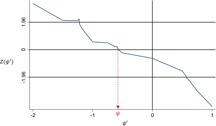
G‐estimation of the causal parameter ψ.

Sometimes, multiple roots may occur, and so the plot in Figure 2 should always be produced to check for this. Although one root could be picked, multiple roots may indicate that the model is unstable, and consideration should be given as to whether results from such an analysis are robust. This may be less of a concern if it occurs very occasionally for samples within a bootstrap to obtain a confidence interval, for example. If selecting one root, some software will pick the one closest to the start of the grid, which may be the most favorable and thus anti‐conservative. Picking the one closest to zero will give the smallest absolute treatment effect which may be preferable, or an average could be taken [4]. Safari et al. [16] discuss some other approaches to handling multiple roots such as changing the grid step size, restricting the grid to a narrower but more plausible range, or using alternative techniques such as iterative parameter estimation (see Section 3.4).

An alternative approach to the grid search is to use interval bisection [13], each time selecting the interval that contains the sign change in the test statistic until a sufficiently small interval for $\mathrm{\psi }$ is obtained. However, multiple roots will not be identified by interval bisection, and can only be evaluated via grid search.

A further helpful model fitting check is to generate the Kaplan–Meier (KM) plot of the counterfactual survival for each arm for the chosen value of $\mathrm{\psi }$, which should look similar. Sometimes even though the test statistic indicates no overall difference in counterfactual survival between arms, the distributions may look quite different (e.g., crossing curves) which may raise some concerns. However, bear in mind that if the test statistic is stratified or adjusted for covariates, the effect of covariates will not be reflected in the KM, which may affect their appearance.

3.3.2. RPSFT Model 2—Final Outcome Model (Compare Adjusted Survival Between Arms)

After estimating $\mathrm{\psi }$ using Model 1, we next compare the observed survival in the experimental arm to the counterfactual survival in the control arm if no switching to experimental treatment had occurred. For control arm switchers, their counterfactual survival ${\mathrm{T}}_{\left\{\mathrm{off},\mathrm{j}\right\}}+{\mathrm{T}}_{\left\{\mathrm{on},\mathrm{j}\right\}}\exp \left(\mathrm{\psi }\right)$ will be different (shorter, if treatment is beneficial) than their observed survival ${\mathrm{T}}_{\left\{\mathrm{off},\mathrm{j}\right\}}+{\mathrm{T}}_{\left\{\mathrm{on},\mathrm{j}\right\}}$; for control arm non‐switchers, their counterfactual and observed survival will be the same (${\mathrm{T}}_{\left\{\mathrm{off},\mathrm{j}\right\}}$). Again, the statistical method used to compare arms should be the same as that used for the observed ITT survival analysis. Kaplan–Meier plots can be directly generated from the adjusted individual patient data. It is also possible to fit flexible survival models to the adjusted data, if extrapolation is the objective.

However, the confidence interval and p‐value that comes directly from this analysis will be incorrect, as unless additional steps are taken to carry through the variability in the estimation of $\mathrm{\psi }$ to the $\mathrm{\psi }$‐adjusted survival analysis, the results will be too precise. $\mathrm{\psi }$ should not be treated as a fixed value.

There are two ways to ensure the variability of $\mathrm{\psi }$ from Model 1 is correctly carried through to the survival analysis result from Model 2. The first and simplest is to maintain the unadjusted ITT p‐value. By combining this with the adjusted point estimate such as the log HR, the correct variability can be obtained for generating confidence intervals that are consistent with that p‐value [19]. The second way is to bootstrap Model 1 and Model 2 together to obtain the bootstrap distribution of the adjusted effect [19, 20]. In general, the first approach should suffice, unless multiple statistical methods need to be applied, or for some reason the same test statistic is not used for the ITT, G‐estimation and final outcomes model. For example, the primary comparison may be a log rank test which should be used to estimate $\mathrm{\psi }$, with the unadjusted p‐value maintained for the RPSFTM p‐value, but if a supportive HR from a Cox model or restricted mean survival difference estimate from a parametric model is also needed then the associated confidence interval could be bootstrapped. Alternatively the log‐rank p‐value could be used to derive the Cox or parametric model based estimate standard error, acknowledging that there would not be a similar correspondence between these quantities in the unadjusted analysis. Bootstrapping can also be helpful when recensoring is applied since the unadjusted ITT result may be affected by recensoring.

It is noted that, although they are both treatment effects and may be similar in magnitude, exp($\mathrm{\psi }$) from Model 1 and the switch‐adjusted hazard ratio from Model 2 have different interpretations and should not be confused with each other. Both models should be executed to obtain the final adjusted hazard ratio.

3.4. RPSFTM Alternatives and Extensions

Iterative parameter estimation [21] (IPE) is very similar to RPSFTM and often gives similar results. The key difference is that $\mathrm{\psi }$ is estimated assuming that the counterfactual survival follows a parametric accelerated failure time distribution, such as a Weibull, and the test statistic Z is based on this. An initial estimate of $\mathrm{\psi }$ is obtained using the observed data, this is used to estimate counterfactual survival for switchers, the arms are compared again, and the process continues iteratively until the estimate of $\mathrm{\psi }$ converges to a prespecified level of precision. Due to the parametric assumption, there will be a unique root. However, RPSFTM is more commonly used as it does not require the additional distributional assumption of IPE. IPE could be a useful sensitivity analysis for RPSFTM if, for example, there are difficulties in finding a unique root.

Bowden et al. [22] propose a weighted version of RPSFTM using a weighted log rank test, which tends to put greater weight on earlier survival times. Jiménez et al. [23] propose using a modified weighted log rank test (as an alternative to RPSFTM) in the presence of switching. These approaches may increase power and precision; thus, the unadjusted p‐value need not be preserved as with RPSFTM. However, a careful justification of the rationale for using alternative weighting would be required.

To adjust for multiple treatments, Xu et al. [24] proposed to either use a random forest model or a stratified version of RPSFTM with multiple levels of subsequent treatment, where the kth subsequent treatment is associated with causal parameter ${\mathrm{\psi }}_{\mathrm{k}}$. The stratified RPSFTM performs a multidimensional grid search over all possible combinations of ${\mathrm{\psi }}_1\prime$ to ${\mathrm{\psi }}_{\mathrm{k}}\prime$, therefore is likely to become computationally intensive as k increases, and may have issues with non‐identifiability of multiple parameters from a single randomisation. It is also likely to require a reasonable number of patients receiving each of the k treatments to avoid model fitting issues. Bell Gorrod et al. [4] provide some further reflections on potential limitations of this method and another “enhanced” RPSFT method proposed by Li et al. [25] for adjusting for two types of switch treatment.

4. Two‐Stage Estimation (TSE)

Two‐stage estimation [2] (TSE) consists of estimating counterfactual survival times for patients who switch treatment, as for RPSFTM, but uses a different statistical methodology to do so.

The TSE adjustment method was originally developed to account for and adjust for treatment switching that occurs at or soon after a particular disease‐related event (such as disease progression), commonly referred as a “secondary baseline”. The counterfactual survival is structured in the same way (see Equation 1) but the acceleration factor is estimated differently. This is done by comparing switchers and non‐switchers from the secondary baseline point, adjusting for important confounders measured at the secondary baseline, that is, treating the second “stage” of the trial after the secondary baseline as an observational study of switching versus not switching. Therefore, a reasonable number of the patients in the subset still at risk at the secondary baseline need to be in the switching and not switching treatment groups for the TSE methodology to be applied, which is a common barrier to its application. Unlike RPSFTM, with TSE the subsequent therapy can be different from that in the other arm of the study; however, due to the requirement that switches only happen at or soon after the secondary baseline, it is often only suited to studies where “crossover” is offered at a pre‐defined point as part of the study design. Similarly, although TSE can be used to adjust for switching occurring in both arms, it is only suitable if both arms are restricted to switch at a specified point, which is not common.

4.1. Assumptions of TSE

The key assumption of the standard TSE model is that there are no important unmeasured confounders; that is, that all of the important covariates that influence both survival and the decision to switch are included in the model comparing post‐secondary baseline survival between switchers and non‐switchers. Identification of potential confounding covariates is discussed further in Section 6.3.

Since only covariates available (or imputed) at the time of secondary baseline are used in the simple TSE model, it is assumed that there is no additional confounding occurring in the time period between secondary baseline and the time of switch. If switch occurs soon after secondary baseline, this assumption should be reasonable. However, if some patients have a longer time period between secondary baseline and switch, this simple TSE method may not be suitable; a potential extension is discussed in 4.4. Defining what length of gap would be acceptable will be study specific and clinical input should be sought; details could be pre‐specified in the protocol.

4.2. Other Considerations When Determining the Suitability of the TSE Model

Many considerations for TSE are similar to IPCW, and we refer the reader to the later IPCW Section 6 on this. Unlike RPSFTM, neither TSE nor IPCW are randomisation‐based methods, and so the adjusted p‐value can differ from the unadjusted p‐value.

An additional consideration for TSE is whether any patients switch before secondary baseline, for example, without confirmed disease progression. Such patients will not be in the risk set at the secondary baseline and may be quite different from those that switch post‐secondary baseline and so, in general, should not be included in the model to estimate the acceleration factor or have their survival adjusted with that acceleration factor. Therefore, their observed survival must be used, without removing the effect of switch treatment. If there are such patients, or at least a non‐negligible proportion, TSE may not be a suitable method. One way to assess their potential influence would be to do two sensitivity analyses, both setting the secondary baseline for these patients as the point of switch, one where their survival is adjusted using the AF from true secondary baseline patients and one where these patients are also included in the estimation of the AF. If either of these was markedly different from the primary analysis, then TSE would not be appropriate. However, such sensitivity analyses should not be over‐interpreted since they are unable to define secondary baseline in the same way for all patients and so these inferences may be biased.

Secondary baseline is typically set as disease progression, but it could be another clearly defined event that would trigger the switch decision. For example, in the PACIFIC study, Ouwens et al. [26] set secondary baseline as initiation of any subsequent therapy and compared patients that switched to immunotherapy versus other therapies (see Section 4.4). However, it is still important that all important confounders are included in the model—for example, if switching were allowed if a patient was unable to tolerate the comparator therapy, the type and severity of that intolerance may influence their switch decision and future outcome. If switching was also allowed at disease progression, then the earlier of those two events would become the secondary baseline, and the type of secondary baseline (progression or intolerance) would likely be an important confounder. Extra care is needed with such a “composite” secondary baseline, since switching patterns and reasons may differ by type of event. Since the standard implementation of TSE applies a single AF to all switching patients, it will be important that the treatment effect does not depend on the type of event. Alternatively, separate AFs could be calculated for the different baseline types, although this will add complexity to the modeling and interpretation. Consideration may need to be given to interactions between secondary baseline type and other confounders. The analyst should check that patients who experience both events (e.g., intolerance followed by disease progression) switch soon after the first; if some switch at the first and some at the second, then the assumption of no unmeasured confounding between secondary baseline and switch may be violated. Analyses which depart from the typical secondary baseline of disease progression should therefore be used and interpreted cautiously.

4.3. How to Fit the TSE Model

As with RPSFTM, before fitting a TSE model, consideration should be given to whether to use recensoring (Section 5), and how to define the time on treatment (${\mathrm{T}}_{\left\{\mathrm{on},\mathrm{j}\right\}}$; Section 3.3).

4.3.1. TSE Model 1—Estimate the Acceleration Factor

For ease of explanation, we focus on subjects switching from control to experimental treatment (and/or other treatments that we wish to adjust for in the control arm). If both arms are being adjusted, this process is repeated to adjust for switching in the experimental arm.

In the first model, focusing only on control arm patients, one compares post‐secondary baseline survival times for patients who switch onto the experimental treatment to those who did not. A parametric AFT model is used (most commonly Weibull, lognormal, log‐logistic or gamma), the distribution being chosen based on the best fit by, for example, AIC or BIC. The model also controls for prognostic characteristics measured at the secondary baseline time point and includes the time‐dependent (usually) switch indicator. The effect of treatment associated with switching can be obtained from there as an acceleration factor (AF). An alternative to including the covariates directly in the model is to estimate a propensity score for switch treatment [26] and use inverse probability of treatment weights to fit weighted parametric AFT models.

Essentially, this represents a simplification of the approach used by Robins and Greenland [27] and Yamaguchi and Ohashi [28] to adjust for treatment switches, in which a structural nested model was utilised to estimate the treatment effect in the control group, rather than a less complex AFT model as suggested here [2].

4.3.2. TSE Model 2—Final Outcome Model (Compare Adjusted Survival Between Arms)

As in RPSFTM, we next use the shrinkage factor (1/AF) from Model 1 to adjust the survival times in the control arm by replacing them with the counterfactual times. If the experimental arm is also being adjusted to remove the effect of switching, we do the same to the experimental arm survival times using the AF from the experimental arm Model 1 fit. Analysis proceeds as for RPSFT Model 2 (Section 3.3.2). As with RPSFTM, Kaplan–Meier plots and models for extrapolation can be fit directly to the adjusted individual patient data.

Again, we must ensure that the variability in the estimation of the AF from Model 1 is carried through to Model 2, or the results from Model 2 will be too precise. This is commonly done by bootstrapping (Model 1 and Model 2 together) [29].

4.4. TSE Extensions

Latimer et al. [29] describe an extension of simple TSE, referred to as TSEgest, to adjust for additional time dependent confounding between secondary baseline and time of switch, via G‐estimation. Simulations showed that this may be a useful alternative approach in some scenarios, particularly when there is time dependent confounding and a high switch proportion which leads to large bias with standard TSE and IPCW. However, this negates one of the main practical advantages of standard TSE over IPCW; namely that the collection of time dependent covariate data after secondary baseline is not required.

Ouwens et al. [26] describe a modified two‐stage method which was applied in the PACIFIC study of durvalumab versus placebo in non‐small cell lung cancer. Standard TSE using progression as a secondary baseline to adjust for the effects of switching to immunotherapy was not applicable as the switch occurred a median of ~6 months after progression. Instead, the start of any subsequent therapy was used as a secondary baseline, and thus the survival time of patients starting immunotherapy was replaced with an estimated counterfactual survival if they had received other therapy (e.g., traditional chemotherapy). This was done sequentially by line of subsequent therapy, first looking at patients who received second or later subsequent therapy and adjusting for immunotherapy based on the start of second or later subsequent therapy as a secondary baseline, and then similarly looking at first subsequent therapy as a secondary baseline.

Some alternative methods that have been proposed for adjusting time to event outcomes for treatment switching, including random forests, regression imputation, semi‐competing risks models, semi‐parametric copula‐based models, decision analytic modeling, and use of external data, are discussed in Bell Gorrod et al. [4].

5. Re‐Censoring in RPSFTM and TSE

RPSFTM and TSE involve calculation of an acceleration factor which represents the prolonging of survival times for those on the control arm, as a result of switching to the (often beneficial) experimental treatment. Crudely applying this acceleration factor to shrink a patient's survival time can result in informative censoring, as a consequence of shrunken censoring times occurring earlier in switchers than non‐shrunken censoring times in non‐switchers, when switch is linked to prognosis. Hence, censoring time is no longer independent of failure time. Censoring is uninformative on the observed time scale, but is informative on the counterfactual time scale. A method called re‐censoring [13] has been proposed to mitigate the effects of informative censoring bias. However, as will be discussed shortly, this also comes at the price of loss of information. As a result of this necessary trade‐off, it requires due consideration prior to implementing.

Re‐censoring involves breaking the dependence between censoring time and switch status (prognosis) by applying a new censoring rule that affects all patients in the same way. Let $C_i$ be the administrative censoring time (data cut‐off) for patient i. All patients still at risk are then censored at the earlier of their observed administrative censoring time or a new administrative censoring time.

Specifically, the counterfactual survival times of patients are re‐censored at their potential censoring time $D_i\left(\psi \right)$, which is the minimum of the administrative censoring time observed or the adjusted administrative censoring time after application of the acceleration factor:

$$D_i\left(\psi \right)=\min \left(C_i,C_i\exp \left(\psi \right)\right)$$ (2)

If switch treatment is beneficial, as is usual, then $D_i\left(\psi \right)<$ $C_i$. If $D_i\left(\psi \right)$ is less than the counterfactual survival time for patient i (whether event or censored), this time is replaced by $D_i\left(\psi \right)$, and re‐censoring occurs, which means the event status of patient i is set to censored. In this way, counterfactual survival times of both switchers and non‐switchers are re‐censored at a common earlier point that is independent of switch status/prognosis, thus eliminating informative censoring.

It is noted that an amendment to the definition of $D_i\left(\psi \right)$ can be used in the situation where no switching can occur for any patient for an initial period of time $F$ in the trial. For example, switching may not be allowed until after results of an interim analysis that occurs at time $F$ after the last subject entered the trial. In that case, only the time after this initial period needs to be adjusted, and we replace $C_i\mathit{exp}\left(\psi \right)$ with $F+\left(C_i-F\right)\mathit{exp}\left(\psi \right)$ in Equation (2). The impact of re‐censoring will be reduced as $F$ increases.

Re‐censoring is applied for data on the counterfactual time scale, and therefore should be applied to all patients in the RPSFTM G‐estimation procedure which compares counterfactual survival between arms to obtain the AF. The exception to this would be if the experimental arm has complete treatment (all patients are on treatment for the entire period, for example, in the “treatment group” approach) (Section 3.3), in which case recensoring is not required in the experimental arm since all patients will be affected by the AF shrinkage equally.

In the subsequent analysis of adjusted survival for both RPSFTM and TSE, observed survival is used for the experimental arm, so recensoring need only be applied to the control arm. For control arm non‐switchers, although their counterfactual survival happens to be equal to their observed survival, re‐censoring still needs to be applied to break the dependency between censoring time and switch status in the control arm. An alternative “hybrid” recensoring approach for RPSFTM, where recensoring is applied in the AF estimation model but not the adjusted survival model, is discussed at the end of this section.

Re‐censoring has been shown to mitigate the problems associated with informative censoring bias; however, it can be associated with missing follow‐up information bias as a result of the shrinkage of survival times and the re‐censoring of events at timepoints earlier than those observed on the trial. The bias associated with missing follow‐up information is apparent when switching to the experimental agent is beneficial for the patient and proportional to the magnitude of benefit seen in the trial—with larger treatment benefits associated with larger acceleration factors and therefore greater shrinkage—shortening the follow‐up time considerably as a result of the shrinkage. This can be seen in examples such as Figure 3, taken from the NICE submission of axicabtagene ciloleucel in relapsed or refractory diffuse large B‐cell lymphoma after first‐line chemotherapy [30]. Here, the last observation for the standard of care therapy (SOCT) RPSFTM adjusted curve with full recensoring in blue is more than 18 months earlier than the SOCT curves for other switch adjustment methods; over half of the follow‐up period has been lost due to recensoring. A similar example from a different study in metastatic melanoma, including TSE, is presented by Latimer et al. [31].

FIGURE 3.

Example of information loss due to full recensoring in RPSFTM (blue curve) in the ZUMA‐7 study of axicabtagene ciloleucel versus standard of care therapy (SOCT) in diffuse large B‐cell lymphoma.

This information loss is often more acute with the “on‐treatment” approach than the “treatment group” approach, as AFs tend to be larger but applied for shorter periods when estimating counterfactual survival (since ${\mathrm{T}}_{\left\{\mathrm{on},\mathrm{j}\right\}}$ stops when switch treatment stops). However, they are applied for the whole trial period when defining potential censoring time, meaning $D_i\left(\psi \right)$ occurs early and lots of information after this point is lost to re‐censoring.

In simulations [31], methods that do not account for re‐censoring have been shown to typically overestimate outcomes in the control group. Therefore, bias was directionally positive in these analyses, whereas methods that re‐censor underestimated to a proportionate degree outcomes in the control arm, therefore had negative biases. However, this is situation specific, and in real‐life studies it is not always the case that analyses without re‐censoring estimate better outcomes for control than those with re‐censoring. The simulated magnitude of bias was different for the different methods (RPSFTM, TSE), with the re‐censoring in RPSFTM typically associated with the largest degree of negative bias. TSE typically had the lowest level of bias associated with it, although this varied according to the magnitude of treatment effect and prognosis of switchers, for example.

Re‐censoring therefore has been cautiously put forward as a way to mitigate biases associated with these two treatment switching methods, as it addresses the issue associated with informative censoring bias; however, this comes at the expense of loss of follow‐up information. There is a lot of conflicting guidance in public literature as to whether to re‐censor or not, and no real consensus on which method provides the least biased results. Latimer et al. [31] recommend presenting results both with and without recensoring. For TSE, an approach combining TSE with IPCW has also been suggested as an alternative for handling informative censoring; simulations [32] showed that it could be useful, but its performance compared to recensoring approaches varied depending on the scenario. In our experience, it is often obvious (from comparing the last data timepoint and number of events after recensoring to the observed data) when recensoring causes a major issue with loss of long‐term follow‐up information. Early truncation of the survival curves due to recensoring may have an impact in terms of increased uncertainty when the adjusted survival curves are extrapolated over a longer time horizon, for example, to use in health economic modeling.

Re‐censoring can also be problematic, as it can lead to model misspecification. As re‐censoring typically involves truncation of the survival curves, estimation of the true treatment effect after adjusting for switch is therefore calculated over a shorter follow‐up duration. Where we would typically assume the effect of experimental treatment to diminish over time, this would lead to an over‐estimation of the true treatment effect when applying re‐censoring. Simulation studies have shown that on account of this, RPSFTM analyses can lead to negative bias; that is, they over‐adjusted for the true impact of treatment switching.

For RPSFTM, a potential alternative to full recensoring or no recensoring is a hybrid approach, where recensoring is applied in the AF estimation model (Model 1) but not the adjusted survival model (Model 2), that is, at the point of estimating $\mathrm{\psi }$ but not the final survival analysis. This approach was used in the NICE submission of osimertinib in metastatic EGFR and T790M mutation‐positive non‐small cell lung cancer [33]. This may have some advantages in reducing informative censoring bias in the estimation of $\mathrm{\psi }$ whilst reducing bias due to information loss in the final survival analysis. However, it does not eliminate the alternative sources of bias in each model. The performance of the hybrid method has not been evaluated in simulations, to our knowledge. Nevertheless, it may be a useful additional approach to present alongside the more usual full and no recensoring results, in scenarios where full recensoring results in a large degree of information loss.

6. Inverse Probability of Censoring Weighting (IPCW)

The inverse probability of censoring weighting (IPCW) method originated in the causal inference literature (as did RPSFTM), and given the assumptions are satisfied, can estimate an unbiased adjusted treatment effect in the presence of time‐varying confounders [9]. Unlike RPSFTM, with IPCW the subsequent therapy can be different from that in the other arm of the study. Both arms can be adjusted, and the therapies adjusted for can be different for the different arms. IPCW differs in approach from RPSFTM and TSE as it does not adjust the individual survival times of patients but instead estimates weights for each patient to define a pseudo‐population.

IPCW extends naïve censoring techniques based on per‐protocol analysis where patients are censored at the time of treatment switching. Naïve artificial treatment censoring at the time of switch introduces informative censoring because the outcomes of patients who switch and those who do not are likely to be different.

In IPCW, the bias associated with informative naive censoring is removed by weighting each patient in the experimental and control arm. The weight for each patient is the inverse of the predicted probability of not being censored (i.e., not switching from planned treatment) at any given time conditional on the observed values of baseline and time‐varying covariates. Uncensored patients are up‐weighted based on the covariate similarity of censored patients [34]. Patients with a low probability of treatment switch (unlikely to switch) are given relatively smaller weights compared to patients with a larger probability of treatment switch. For example, if patients with higher biomarker expression are more likely to switch, patients with higher biomarker expression who have not yet switched are assigned higher weights. By applying this IPC weighting, the differences between censored switchers and uncensored non‐switchers should be eliminated and censoring becomes uninformative, removing the bias associated with the naive censoring approach.

6.1. Assumptions of IPCW

The main challenge in applying IPCW is to establish that the weights adjust appropriately for the bias created by censoring switchers, such that the covariates available at baseline and over time include all important ones that are prognostic for survival and influence the probability of treatment switching [18]. This is the “no unmeasured confounders” assumption that also applies to TSE as previously described in Section 4.1; we can never be sure that we have no unmeasured confounders. Although this is the same assumption as for TSE, for IPCW we can use covariates over the entire study time period to satisfy this assumption, not just those at secondary baseline.

6.2. Other Considerations When Determining the Suitability of the IPCW Model

Unlike RPSFTM, IPCW is not a randomisation‐based method, and so the adjusted p‐value can differ from the unadjusted p‐value.

Since Model 1 of the IPCW method (see Section 6.4.1) compares switchers and non‐switchers within an arm, there needs to be a reasonable number of patients in both of these groups to obtain robust model estimates. So if the proportion of switchers is very high, IPCW will not be suitable; if it is very low, there is little point in adjusting for switch (indeed, this applies to all methods). Simulations [2, 18] have shown IPCW is prone to substantial error if more than 85% of patients switch in a control arm of 250 patients; however, it will also depend on absolute numbers, and smaller studies may be affected at lower switching proportions. Further simulations [14] have suggested that all methods provide close approximations of the true treatment effect when the switching proportion is moderate, defined as less than approximately 60% of the patients eligible to switch. Therefore, we propose that IPCW is best suited to switching proportions of 40%–60%, unsuitable with switch proportions over 85% or under 15%, and used cautiously in other situations, particularly in smaller studies. If there are certain preconditions that need to be met prior to switch being possible (e.g., it is only offered to patients still in the study following an interim analysis, or who have disease progression), then the proportions and group sizes should be assessed in the subset of patients eligible for switch. The same principle applies to TSE, where this should be assessed in the patients with a secondary baseline.

It is expected that there will be at least one time‐varying covariate in an IPCW model, since it is likely that something has changed over time since baseline that has influenced the decision to switch at that point, such as disease worsening. If switch truly only depends on baseline factors then a simpler model can be applied, but such a situation seems unlikely.

The IPCW method is not suitable if there are any covariate patterns which predict with probability equal to one that treatment switching will take place [35]. Additionally, those with probabilities close to one are likely to lead to model fitting difficulties. This means that if there are any important confounding variables that are observed exclusively or near‐exclusively in switchers (or non‐switchers)—for example all/most patients with disease progression chose to switch—then IPCW will not be appropriate. Similar considerations will apply in TSE.

Furthermore, the correctness of model specification is important: Model 1 (weight determining model) and Model 2 (final outcome model to compare adjusted survival data) need to be correctly specified to lead to reasonable bias reduction in the trial.

6.3. Covariate Selection for IPCW and TSE

A suggested approach to defining a set of potentially confounding covariates to adjust for in the IPCW and TSE models is provided in the Data S1.

6.4. How to Fit the IPCW Model

As with RPSFTM and TSE, there are two models in IPCW.

6.4.1. IPCW Model 1—Estimate Weights

At first, a switching model is defined within an arm to estimate the probability that the patient has not yet switched by time t, dependent on baseline and time‐varying covariates. If both arms are being adjusted for subsequent therapies, separate models are typically fitted for each arm, unless the switching behavior can reasonably be expected to be the same for each arm (e.g., the switch therapy is the same and the impact of covariates on the decision to switch does not differ by randomised arm). A patient will be censored at treatment switch and is removed from the at‐risk set.

We wish to fit a time dependent Cox model which typically has a form as shown in Equation (3) [9], where h _C is the arm‐specific hazard of switch (censoring), $\overline{V}\left(t\right)$ is past covariate history, T is the actual switch time, h ₀ is the arm‐specific baseline hazard, and $V\left(t\right)$ is the baseline and current time varying covariate values:

$$h_c\left\{t|\overline{V}\left(t\right),T>t\right\}=h_0\left(t\right)\exp \left\{\alpha \prime V\left(t\right)\right\}$$ (3)

It is noted that, if desired, the analyst may change the form of this model such as incorporating more complex interactions between covariates or with time; the proportional hazards assumption is discussed further in Section 7. However, the model is structured, we then use this to estimate the probability of switch for each subject and each time at risk, which we then convert into an inverse probability of switch (censoring) weight.

There are two modelling approaches that can be used. We can fit the continuous time Cox model directly, or we can use a discrete time pooled logistic regression model, which should be a good approximation to this under the assumption that the probability for the event is small in the discrete time interval [36]. When this methodology was first proposed, some software could not handle time‐varying subject‐specific weights from the Cox models. So older examples of IPCW tend to use pooled logistic regression for both estimating weights in Model 1 and performing weighted survival analyses in Model 2. Due to the increased availability of suitable software (see Section 8.2), the time‐dependent Cox model is now more commonly fitted directly rather than using the pooled logistic regression model approximation. However, we discuss both methods here for completeness.

6.4.1.1. Handling Missing Data for Covariates

A covariate value is needed for every patient in every time interval where they are at risk to keep them in the analysis set. Potential strategies for handling missing covariate data are discussed in the Data S1.

6.4.1.2. Estimating Weights From a Time Dependent Cox Model

Firstly, the data is restructured into time intervals with breaks at the appropriate event/switch/covariate change times, as described by Graffeo et al. [37]. For each patient, their event status, switch status, and baseline and time‐varying covariate values are set for each interval and should be constant within that interval. Intervals after switch are removed, which is equivalent to censoring at switch. Intervals after death or censoring for the outcome are also removed.

A time‐dependent Cox model for the hazard of switch over time, dependent on baseline and time varying covariates, can then be fit to the restructured data using the counting process approach as described in Section 8.2.

Each individual's unstabilised IPC weights over time are then obtained from this model (see Graffeo et al. [37] Equation (1)). At a given time t, this weight is defined as the inverse of the probability of remaining unswitched until time t, given the observed values of the baseline and time‐varying covariates at t.

6.4.1.3. Estimating Weights From a Pooled Logistic Regression Model

As with the Cox model, the data are firstly restructured into time intervals, event/switch/covariate values are determined in each interval and post‐switch/event/censoring intervals are removed. Commonly in pooled logistic regression, fixed length intervals are used, but this is not mandatory.

A logistic regression model is fit to each interval for the log‐odds of switch dependent on baseline and time‐varying covariates. Due to the large number of intervals, to reduce the number of parameters compared to fitting a separate intercept for each interval, a smooth function such as a natural cubic spline can be applied to the intercept [38, 39]. For spline expansions, a decision is needed regarding the number and position of the knots to be placed [11]. Hence, pooled logistic regression implementations may require more user judgment in the implementation than the Cox model.

Individual probabilities of switching (censoring) over time based on all covariates V, $P_{C,i}^{\left(V\right)}\left(t\right)$, are then obtained from the model predicted probabilities. The inverse of these, $w_{i,\mathit{\text{unstab}}}=1/P_{C,i}^{\left(V\right)}\left(t\right)$, are the unstabilised IPC weights.

6.4.1.4. Assessing and Stabilizing Weights

Large unstabilised weights can occur, especially towards the end of the observation time when most patients have either experienced the event or have been censored. Alternatively, stabilised weights can be applied which form a narrower distribution with decreased weight variability and increased statistical efficiency [38]. In the weight calculation the numerator is replaced by $P_{C,i}^{\left(B\right)}\left(t\right)$ which is the individual's estimated probability of switch with only the subset of baseline covariates B in the model, rather than the full set of baseline and time varying covariates V. Hence, stabilised weights are $w_{i,\mathit{\text{stab}}}=P_{C,i}^{\left(B\right)}\left(t\right)/P_{C,i}^{\left(V\right)}\left(t\right)$. However, these may not fully resolve the issue of large weights.

The distribution of the weights should therefore be reviewed. Graffeo et al. [37] propose a plot of truncated log‐stabilised weights with a boxplot for each time interval since enrolment. However, within a model that includes a large number of intervals, it may be preferable to plot all weights on the y‐axis over all time intervals and patients on the x‐axis and scan for extreme weights. In the case of a strong covariate‐treatment association, weights estimators may still be considerably variable and positively skewed [40]. For this scenario, truncation may be considered where extreme weights are replaced by minimum and maximum weights according to percentiles of weight distribution, for example, the 95th percentile. Truncation of weights is further discussed in Bell Gorrod et al. [4]. Estimated weights that are extreme in value or that in aggregate do not have a mean close to 1 may indicate model misspecification or non‐positivity, and an estimate of survival based on such weights may fail to correct for bias [41].

6.4.2. IPCW Model 2—Compare Adjusted Survival Between Arms

Once the weights for all time intervals in the counting process are estimated across all patients, these weights can be incorporated within an outcomes model. If only one arm is being adjusted, the weights should be set to 1 in the other arm. The outcomes model can be a weighted Cox model with subject‐specific time‐varying weights, applied using the same counting process approach and time intervals as described for Model 1, modeling the hazard of the outcome event (e.g., death) dependent on treatment arm. Or it could be a weighted pooled logistic regression model, with weights set for each patient in each interval, modeling the log odds of the outcome event in a similar way. It is also possible to fit weighted flexible survival models if extrapolation is the objective. As well as treatment arm, if stabilised weights are used, any baseline confounders from the weight determining model should also be included as covariates in the weighted outcomes models. This is because stabilised weights do not adjust for confounding by baseline covariates, as they are included in both the numerator and denominator of the weight [42].

Confidence intervals generated by this weighted model will be inappropriate because the standard errors are not valid. Weights are estimated in IPCW and are not fixed and known, so the variability in this estimation from Model 1 should be carried through to Model 2. The weights also induce within‐subject correlation. To account for within‐subject correlation, standard errors must be calculated in a robust way, such as using the sandwich variance [38]. To account for the estimation of the weights, bootstrapping can be applied [3]. The whole routine of estimating weights and computing the final outcome model should be bootstrapped simultaneously. A weighted analysis is less efficient (with bigger standard errors) than an unweighted analysis; for example, IPCW is performed to decrease bias, not to gain efficiency.

7. Proportional Hazards Assessment After Switch Adjustment

If necessary, the assumption of proportional hazards after switch‐adjustment can be assessed using standard graphical methods. However, the properties of the various tests that are commonly used for proportional hazards assessment are not fully understood when applied to switch‐adjusted results; this is a potential area for future research. Care should be taken to ensure that any test‐based approaches or confidence bands are using the correct variability.

The IPCW method was developed using the Cox model as a basis, which makes the proportional hazards assumption. It may be possible to adapt this to use, for example, an accelerated failure time distribution‐based parametric model if the alternative assumption about the parametric distribution is deemed reasonable. However, if the unadjusted analysis shows strong evidence of non‐proportional hazards, caution should be exercised when using any of the switch adjustment methods described here, as their performance may be impacted. For example, the common treatment effect assumption of RPFSTM is less likely to hold in this situation.

8. Software and Programming Guidance

Some efforts have been made to develop packages and code in various statistical software to implement treatment switching methods. These are described in this section.

To support analysts who wish to use these models, we have developed a repository of R code applied to a worked example. Details are provided in the Code Appendix at the end of this paper (Section 12).

8.1. RPSFTM and IPE

For RPSFTM, the Stata package strbee [13] was originally developed in 2002 and for a long time remained the only well‐known published option. This can also be used for IPE models. It has many helpful features that enable multiple types of RPSFT models to be fitted.

The rpsftm package [43] in R was released in 2018, and has much of the same functionality as strbee. Time on and off treatment for an individual is represented in the rpsftm() function call using rx, the proportion of total time spent on treatment. The test used for G‐estimation can be based on log‐rank, Cox regression, or parametric survival models and covariates or strata can be included. Recensoring can be applied through specifying the censor_time argument; setting autoswitch = TRUE will not recensor an arm if it is completely treated (rx = 1 [or 0] for all patients). It is also possible to use the treat_modifier argument to conduct sensitivity analyses where $\mathrm{\psi }$ differs by treatment arm, that is, reduced effect in control arm switchers (${\mathrm{s}}_{\mathrm{j}}$ < 1 per Section 3.1) compared to those randomised to treatment.

Outputs include $\mathrm{\psi }$ and counterfactual survival times for both arms, and plots of these can be easily produced. Subsequent modelling of adjusted survival (Model 2 in the earlier section) can then be programmed by the analyst according to their requirements, ensuring that the variability of $\mathrm{\psi }$ is correctly carried through as discussed previously—for example via rearranging the test statistic (formed of the adjusted log HR estimate and its variability) corresponding to the unadjusted p‐value to obtain the adjusted log HR variability, or bootstrapping.

It is noted that, in the case of multiple roots found for the estimation of $\mathrm{\psi }$, the rpsftm package uses the first root in the interval in subsequent calculations (such as generating individual counterfactual survival times). The analyst should consider if this is appropriate for their objective, as discussed earlier in Section 3.3.1, and if necessary, modify their code to use an alternative root.

For RPSFTM in SAS, analysts often write their own code. A macro for estimating $\mathrm{\psi }$ using G‐estimation has been developed by Danner and Sarkar [44]. They show consistent results to the R rpsftm outputs in their example, although they mention it is less efficient. This was based on the log‐rank test and has more recently been extended [45] for Weibull and Cox models. However, the authors of this paper do not yet have experience with the macro and analysts should ensure it is validated for the circumstances of their analysis.

8.2. IPCW

Our original publication [1] describes some approaches that have been used previously to fit IPCW models in Stata and SAS. At the time, the pooled logistic regression approach was commonly used, as described earlier in Section 6.4.1. However, it is now more usual to directly fit a Cox model using a counting process notation [46, 47] for time‐varying covariates in the estimation of IPC weights, and for the weights themselves in the subsequent weighted survival analysis. Start and stop times tstart and tstop are input to define the intervals in which the covariates or weights are constant (see Table 1).

TABLE 1.

Programming syntax for IPCW Cox models in R and SAS.

Software: function	Counting process for IPC weight model (Model 1)	Robust standard errors for weighted survival analysis (Model 2)
R: coxph	Surv(tstart, tstop, switch) ~ <covariates>	Surv(tstart, tstop, event) ~ arm + cluster(subjid), data = dat, weights = ipcw
SAS: PROC PHREG	model (tstart, tstop)*switch = <covariates>	data=dat covs(agg); class arm; model (tstart, tstop)*event=arm; freq ipcw/notruncate; i d subjid;

Event occurrence covariates such as time‐varying progression status or specific adverse events can be set up as indicator variables, taking a value of 0 until the event occurs when the value changes to 1. Switch status is similarly constructed, with the value changing from 0 to 1 in the switching interval. Post‐switch intervals are removed.

Much of the effort in fitting IPCW models comes from manipulating the data into this interval structure. The R package ipcwswitch [37] provides some useful functions for assisting with this process, as illustrated in its accompanying publication. Users should be aware that some functions require quoted arguments when others do not, and that the functions used earlier in the process can use dates, but the later ones require this to be converted to a numeric time since baseline. Some functions may not work or may restructure data incorrectly if datasets are not sorted in the expected order (e.g., by subject identifier) or variables are not in the correct format (e.g., arm as a factor). Therefore, the generated datasets should be very carefully checked. The package also includes a function ipcw() to generate the stabilised (and optionally truncated) IPC weights from time‐dependent Cox models once the data structure is established. It is noted that this function contains a loop which can make it time consuming to run, particularly in a large bootstrap sample; the user may wish to re‐write some parts of it to increase efficiency if needed.

The R package ipw [48] is an alternative that can fit a wider range of marginal structural models. The ipwtm() function with family='survival' can similarly be used to generate IPC weights from a time‐dependent Cox model once data has been structured to meet its requirements. It has some small methodological differences to the ipcwswitch::ipcw() function, which means estimated weights will not always be exactly equal from the two packages [37]. ipw::ipwplot() is useful to plot and explore the weights distribution of any dataset, including those generated by other packages.

Mosier [45] describes a process including a macro for conducting an IPCW analysis based on the Cox model rather than pooled logistic regression in SAS. However, the authors of this paper do not yet have experience with implementing this or how it compares to results from the above R packages; analysts should ensure it is validated for the circumstances of their analysis.

It is recommended to conduct the following programming quality control (QC) check for IPCW analyses, which can highlight any errors in the data re‐structuring or model fitting process: set all the weights in each interval to 1 and re‐run the survival model. The results should match those from a naïve survival analysis where patients are censored at switch.

One advantage of using R rather than SAS to fit IPCW models is the ease with which it produces IPC weighted KM curves in a single line of code—the same counting process syntax can be applied in the survdiff() call as in coxph() to apply time‐varying, subject‐specific weights. PROC LIFETEST in SAS does not currently have this functionality, even though PROC PHREG does. It is further noted that for parametric models in R, flexsurvreg allows counting process syntax but survreg does not. Since IPCW is a weighted analysis, the KM numbers at risk across time will not be integers, although they may be rounded for presentation.

As previously discussed, it is important to carry through the variability in the IPC weight estimation into the weighted survival analysis. This can be done via bootstrapping.

Counting process models may generate error messages when a subject dies, is censored for death, or switches on the same day as baseline (time tstart for the first interval)—for example, if they die on the day of randomisation. This is because the length of the first interval becomes zero days. This can be fixed without affecting the estimated hazard ratio by adding 1 day to all times relative to baseline (death/censoring, switch, data cut off, time‐varying covariate change times) or by adding 0.5 days to any death/censoring/switch times occurring on the same day as baseline [49].

8.3. Two Stage Estimation

At present, there are no known packages or macros specifically for TSE, as this tends to use a combination of already established methods. Some of the approaches described above for IPCW can be applied when writing code for TSE. R code for a worked example is provided in the repository that accompanies this paper.

9. Reporting Recommendations

Sullivan et al. [20] reviewed the quality of reporting on the implementation of switching adjustment methods in oncology trials as reported in published literature and NICE HTA submissions. The authors noted that the quality of reporting was generally poor; for example, few studies discussed whether the adjustment method was pre‐specified, why a particular method had been chosen, how the methods were implemented, and whether any sensitivity analyses were applied to probe assumptions. These limitations made it difficult to assess the validity of the adjusted treatment effect estimates. Bell Gorrod et al. [4] performed a review of recent NICE TAs and similarly found sub‐optimal reporting and reviewing and proposed their own detailed reporting guidelines. Hence, motivated by the authors' recommendations to improve reporting, we present additional modified checklists for outputs common to all treatment switching adjustment methods in Table 2 and further outputs specific to a given adjustment method in Table 3.

TABLE 2.

Reporting checklist for general outputs—all treatment switch adjustment methods.

1	Discuss whether assumptions are plausibly satisfied for treatment adjustment methods.
2	Outline treatment‐switching mechanism: Who could switch and when during study? Optionally, report intercurrent events in the estimands framework following Manitz et al. table 1 [5], for example, distinguishing intercurrent event strategies for switches to investigational drugs and drugs available in a given market.
3	Report number of switchers, when switching occurred and how many were eligible to switch.
4	If covariates adjusted for: What covariates, how they are selected, amount of missingness, and are they fixed or time‐varying covariates? Process for variable selection (targeted literature review, clinical consultation, statistical variable selection etc.).
5	Was the selected adjustment approach (including model fitting steps) pre‐specified?
6	Is the proportional hazard assumption satisfied? How does it influence the choice of final outcome model?
7	Report results from unadjusted and treatment switching adjusted data, such as Kaplan–Meier curves and estimate of the hazard ratio and/or acceleration factor along with their confidence intervals. Outline sensitivity analyses probing some of these key assumptions (e.g., vary covariates in IPCW/TSE, reduce treatment effect for switchers in RPSFTM).

TABLE 3.

Reporting checklist for outputs specific to treatment switching adjustment method.

	IPCW	RPSFTM	TSE
Model 1: Weight or causal parameter estimation	Are weights calculated using Cox model or pooled logistic regression? Are stabilised weights used? Does weight distribution look reasonable and is positivity assumption (switchers and non‐switchers in every patient subset) satisfied? Have weights been truncated?	What structural model is assumed (e.g., treatment group, on treatment)? What hypothesis test (e.g., log‐rank) has been used to derive causal parameter? Were any additional covariates or strata included? What grid‐search algorithm has been used? Are there multiple roots? Which G‐estimation diagnostics have been used (counterfactual KM‐curves, plot of Z($\mathrm{\psi }\prime$) vs. $\mathrm{\psi }\prime$)? Has re‐censoring been applied?	What structural model is assumed (e.g., treatment group, on treatment)? How is the secondary baseline defined? How many days after secondary baseline is the subsequent therapy start date? Have any variations to simple TSE been applied? Which AFT model has been applied? Is the AFT model (e.g., Weibull, Gompertz) fixed or selected using model selection?
Model 2: Final outcomes	Is a Cox model or pooled logistic regression used? Were any additional covariates or strata included? Has the uncertainty in weights been accounted for, for example, by bootstrapping?	Were any additional covariates or strata included? Has re‐censoring been applied? Has the uncertainty in the causal parameter estimation been accounted for, for example, inflating standard errors to preserve the unadjusted ITT p‐value or bootstrapping?	Were any additional covariates or strata included? Has re‐censoring been applied? Has the uncertainty in the causal parameter estimation been accounted for, for example, by bootstrapping?

10. Acceptance of Treatment Switching Methods by Regulatory and HTA Agencies

Trial designs that exclude the option of crossover to the investigational arm therapy are generally preferred from a methodological standpoint [3]. The European Medicines Agency (EMA) explicitly advises against the inclusion of crossover at the time of progression unless detrimental effects on overall survival have been ruled out [50]. However, it is not always possible to exclude crossover for practical or ethical reasons, and even if that is excluded, then patients often switch to other therapies. When crossover or treatment switch occurs, a strategy is required for handling this in the analysis.

Pivotal clinical trials are primarily designed to demonstrate that a treatment is efficacious and safe, in order to obtain regulatory agency approval. Traditionally, such trials have been analysed using the principle of intention to treat (ITT) after it was included into the ICH E9 guideline on the “Statistical Principles for Clinical Trials” in 1998 [51]. ITT does not make any adjustments to the estimate due to switching. It has long been recognised that for health technology assessment (HTA) and approval for reimbursement, it is most relevant to estimate the effect of treatment if used in clinical practice in the region of interest, and that this may differ from the primary estimate from the pivotal trial(s). In other words, the estimands of interest for HTA and regulatory agencies are often different. Therefore, the use of treatment switching methods has been more widely used in HTA than regulatory settings, to address a hypothetical estimand that removes the effect of therapies taken in the trial that are outside the standard clinical pathway for that region.

However, there is increasing attention to the effect of treatment switching in a regulatory setting too. The ICH E9 (R1) “Addendum on Estimands and Sensitivity Analysis in Clinical Trials to the Guideline on Statistical Principles for Clinical Trials” [52], released in 2020, discusses that for certain intercurrent events (ICEs), which may include treatment switch, there might be interest to depart from the intent‐to‐treat principle (also known as the “treatment policy” strategy for handling ICEs). This would depend on the estimand. The regulatory interest in hypothetical estimands, as per ICH E9 (R1), is considered limited, although it is acknowledged in scenarios where intercurrent events or their consequences differ between clinical trials and clinical practice. Consequently, analyses using treatment switching methods currently tend to play a supplementary role in regulatory submissions. For example, RPSFTM adjusted survival analyses were discussed as supportive evidence at the September 2022 FDA advisory committee meeting for PB‐TURSO in amyotrophic lateral sclerosis [53].

Moreover, even in HTA, there are variations between agencies in the degree of acceptability of switch adjustment methods, due to the additional assumptions involved and the differing agency decision‐making processes. Treatment switch can have a substantial impact when a cost‐effectiveness model with a long‐term time horizon is used in the reimbursement decision criteria. The UK (NICE) and Australian (PBAC) agencies, which take a cost‐effectiveness perspective, have published extensive guidance on these methods [3, 4, 54]. There are several examples of NICE accepting adjustment methods, provided the methods used are appropriate [30, 55, 56, 57, 58, 59]. The use of adjustment methods in analyses has led to modifications in reimbursement decisions for certain procedures [60, 61]. A notable instance is the comparison of sunitinib and best supportive care for the treatment of gastrointestinal stromal tumors, where the Incremental Cost‐Effectiveness Ratio (ICER) varied by a factor of three between RSPFTM vs. ITT analyses [56].

At the opposite end of the spectrum, the German Institute for Quality and Efficiency in Health Care (IQWIG), which does not consider cost effectiveness criteria, does not accept such evidence [62]. IQWIG published a working paper on treatment switching in oncological studies [63] concluding that currently available statistical methodology does not allow analysis of trials with treatment switching with sufficient confiden as the application of treatment switching methods carries the risk of biased evaluation due to untestable assumptions. This aligns with IQWIG's general preference for ITT analyses disregarding treatment discontinuation or switch. Morga et al. [60] offer a comprehensive review of the distinct perspectives on estimands from NICE and IQWIG.

Most remaining HTA agencies do not have a documented position; for example, the Canadian Agency for Drugs and Technologies in Health (CADTH) does not explicitly mention treatment switching methods in their guidance document [64]. Considering that the EU joint clinical assessment started in early 2025 for oncology products, EUnetHTA has issued numerous methodological guidance documents that have been adopted by the European Commission. However, there appears to be no attempt to harmonise this particular topic across member states for future HTA submissions, despite explicit requests for recommendation as per the public consultation comments [65, 66].

11. Summary and Conclusions

This paper endeavors to bring together multiple sources of information about adjusting long‐term outcomes for the effect of treatment switching, to provide a useful summary of the current situation regarding their use and practical application. By the nature of such a topic that is constantly under research and evolution, it is not an exhaustive review, and the analyst should remain alert to new developments since publication.

As discussed in Section 2, it is very important to have a clear clinical question of interest or estimand [5] before starting to plan the analyses, and to be aware that this may differ for different review bodies. Therefore, multiple treatment switching analyses may be required for a study to address different estimands. Even within an estimand, multiple analyses are still likely to be required to assess sensitivity to violation of assumptions with the method used, or the impact of using alternative methods. Therefore, we recommend writing an analysis plan and obtaining cross‐functional input prior to commencing analyses, even if these are being conducted post hoc. Not only will this clarify thinking, it will also highlight the extent of the work involved, which is often considerable.

We focussed on the three most commonly applied complex methods for addressing a hypothetical estimand with a differing switch pattern to that observed in the trial: RPSFTM, TSE, and IPCW. The key features of these methods are summarised in Table 4. Other methods are available, and several of them are briefly addressed in this paper.

TABLE 4.

Key features of rank preserving structural failure time models (RPSFTM), two‐stage estimation (TSE), and inverse probability of censoring weighting (IPCW) methods.

	RPSFTM	TSE	IPCW
Type of switch treatment that can be adjusted for	Treatment in the other arm (“crossover”), or treatments expected to have the same effect	Any, if switch only occurs at or soon after secondary baseline, for example, progression (for simple TSE)	Any
Amount of switching (amongst those eligible for switch) that can robustly be adjusted for	Any (although unlikely to have much impact if low, e.g., < 15%)	Moderate a	Moderate a
Key assumptions	Common treatment effect Same outcome in each arm if treated the same (prognostic covariates balanced)	No unmeasured confounding (all important baseline and secondary baseline covariates that influence outcome and switch are included in the model) No additional confounding between secondary baseline and switch (for simple TSE)	No unmeasured confounding (all important baseline and time‐varying covariates that influence outcome and switch are included in the model)
Data collection requirements, beyond randomised arm, observed event time, and switch treatment start time	Switch treatment stop time if using “on‐treatment” approach	Switch treatment stop time if using “on‐treatment” approach Potential confounding covariate values up to and at secondary baseline	Potential confounding covariate values at all times until switch, event, or censoring
Analysis approach—key decisions	Recensoring—full, none, hybrid Definition of time on treatment—treatment group or on‐treatment How to account for all variability—preserve ITT p‐value or bootstrap	Recensoring—yes, no Definition of time on treatment—treatment group or on‐treatment Identification of potential confounders to adjust for Definition of secondary baseline Parametric AFT model distribution How to account for all variability—bootstrap	Identification of potential confounders to adjust for Time dependent Cox model or pooled logistic regression How to account for all variability –bootstrap
Problematic scenarios	Small ITT treatment effect (unlikely to change with adjustment) Similar time on experimental treatment between arms (model fitting difficulties) Reassessment of statistical significance is desired (p‐value preserving method)	Gap between secondary baseline and switch (violation of assumption) Patients switching before secondary baseline (inconsistent with model structure) Covariates that are perfect or near‐perfect predictors of switch (model fitting difficulties)	Early cessation of collection of time varying confounders (violation of assumption) Covariates that are perfect or near‐perfect predictors of switch (model fitting difficulties)

^a We propose switching proportions of 40%–60%, unsuitable with switch proportions over 85% or under 15%, and used cautiously in other situations, particularly in smaller studies.

In particular, we would like to emphasise the importance of ensuring all sources of variability are carried through into the final estimate of the switch‐adjusted treatment effect. The results from the final adjusted survival model (Model 2) should be adjusted to account for the additional variability from the previous modeling of the weights or acceleration factor (Model 1). We have seen several examples where this has not happened, leading to switch‐adjusted p‐values that are too small and confidence intervals that are too narrow.

Since our initial publication in 2013 [1], the availability and functionality of software code for treatment switching analyses has greatly improved, as discussed in Section 8. However, there are still areas where this could be improved, for example, the availability of validated macros in SAS and worked examples of code published for the TSE method. A repository of R code has been developed to accompany this paper.

Another area for potential improvement is around reporting of treatment switching analyses, as highlighted by Sullivan et al. [20] and Bell Gorrod et al. [4]. In Section 9, we suggest some modified reporting checklists that highlight some of the statistical nuances that a diligent statistician should include in a report.

Looking to the future, analyses adjusting for treatment switching seem set to continue to play a key role in assessing if a drug is efficacious and cost effective. More treatments are becoming available, providing more opportunity to switch, and trials often offer control arm patients the opportunity to switch to the investigational therapy as a recruitment incentive. Thus, switching affects overall survival and other long‐term outcomes in many trials. A greater awareness of the influence of treatment switching as an intercurrent event has been generated with the publication of the ICH E9 addendum [52] and future estimands may increasingly require some adjustment for that, for either regulatory or HTA purposes. It is unfortunate that the current EUnetHTA guidance does not explicitly address this important topic. However, we hope that analysts find this paper a useful resource when planning and conducting analyses adjusting for treatment switching.

12. Code Appendix

To support analysts who wish to use these models, we have developed a repository of R code. This works through how to apply RPSFTM, IPCW, and TSE methods to a worked example, step by step from start to finish. This is available at the link: https://bitbucket.org/clairewatkins/trtswitch_samplecode_share/src/main/.

Please cite this publication when applying the code. Any bugs, issues, or suggestions for code development can be shared with the primary author at claire.watkins@clarostatconsulting.com.

Conflicts of Interest

The authors declare no conflicts of interest.

Supporting information

Data S1. Supporting Information.

Watkins C., Kleine E., Miranda M., Bourmaud E., and Doehring O., “Further Practical Guidance on Adjusting Time‐To‐Event Outcomes for Treatment Switching,” Pharmaceutical Statistics 24, no. 4 (2025): e70019, 10.1002/pst.70019.

Data Availability Statement

Data sharing is not applicable to this article as no new data were created or analyzed in this study.

References

- 1. Watkins C., Huang X., Latimer N., Tang Y., and Wright E. J., “Adjusting Overall Survival for Treatment Switches: Commonly Used Methods and Practical Application,” Pharmaceutical Statistics 12, no. 6 (2013): 348–357, 10.1002/pst.1602. [DOI] [PubMed] [Google Scholar]
- 2. Latimer N. R., Abrams K. R., Lambert P. C., et al., “Adjusting for Treatment Switching in Randomised Controlled Trials—A Simulation Study and a Simplified Two‐Stage Method,” Statistical Methods in Medical Research 26, no. 2 (2017): 724–751, 10.1177/0962280214557578. [DOI] [PubMed] [Google Scholar]
- 3. Latimer N. R. and Abrams K. R., “NICE DSU Technical Support Document 16: Adjusting Survival Time Estimates in the Presence of Treatment Switching.” 2014, http://www.nicedsu.org.uk. [PubMed]
- 4. Bell Gorrod H., Latimer N. R., and Abrams K. R., “NICE DSU Technical Support Document 24: Adjusting Survival Time Estimates in the Presence of Treatment Switching: An Update to TSD 16.” 2024, http://www.nicedsu.org.uk. [PubMed]
- 5. Manitz J., Kan‐Dobrosky N., Buchner H., et al., “Estimands for Overall Survival in Clinical Trials With Treatment Switching in Oncology,” Pharmaceutical Statistics 21, no. 1 (2022): 150–162, 10.1002/pst.2158. [DOI] [PubMed] [Google Scholar]
- 6. Mattei A., Ding P., Ballerini V., and Mealli F., “Assessing Causal Effects in the Presence of Treatment Switching Through Principal Stratification. arXiv Preprint arXiv.” 2020, 2002.11989.
- 7. Latimer N. R., Bell H., Abrams K. R., Amonkar M. M., and Casey M., “Adjusting for Treatment Switching in the METRIC Study Shows Further Improved Overall Survival With Trametinib Compared With Chemotherapy,” Cancer Medicine 5, no. 5 (2016): 806–815, 10.1002/cam4.643. [DOI] [PMC free article] [PubMed] [Google Scholar]
- 8. Hardy W. D., Feinberg J., Finkelstein D. M., et al., “A Controlled Trial of Trimethoprim‐Sulfamethoxazole or Aerosolised Pentamidine for Secondary Prophylaxis of Pneumocystis Carinii Pneumonia in Patients With the Acquired Immunodeficiency Syndrome. AIDS Clinical Trials Group Protocol 021,” New England Journal of Medicine 327, no. 26 (1992): 1842–1848, 10.1056/NEJM199212243272604. [DOI] [PubMed] [Google Scholar]
- 9. Robins J. M. and Finkelstein D. M., “Correcting for Noncompliance and Dependent Censoring in an AIDS Clinical Trial With Inverse Probability of Censoring Weighted (IPCW) log‐Rank Tests,” Biometrics 56, no. 3 (2000): 779–788, 10.1111/j.0006-341x.2000.00779.x. [DOI] [PubMed] [Google Scholar]
- 10. Paganoni S., Hendrix S., Dickson S. P., et al., “Long‐Term Survival of Participants in the CENTAUR Trial of Sodium Phenylbutyrate‐Taurursodiol in Amyotrophic Lateral Sclerosis,” Muscle & Nerve 63, no. 1 (2021): 31–39, 10.1002/mus.27091. [DOI] [PMC free article] [PubMed] [Google Scholar]
- 11. Dodd S., Williamson P., and White I. R., “Adjustment for Treatment Changes in Epilepsy Trials: A Comparison of Causal Methods for Time‐To‐Event Outcomes,” Statistical Methods in Medical Research 28, no. 3 (2019): 717–733, 10.1177/0962280217735560. [DOI] [PMC free article] [PubMed] [Google Scholar]
- 12. Robins J. M. and Tsiatis A. A., “Correcting for Noncompliance in Randomised Trials Using Rank Preserving Structural Failure Time Models,” Communications in Statistics ‐ Theory and Methods 20 (1991): 2609–2631. [Google Scholar]
- 13. White I., Walker S., and Babiker A., “Strbee: Randomisation‐Based Efficacy Estimator,” Stata Journal 2, no. 2 (2002): 140–150. [Google Scholar]
- 14. Latimer N. R., Abrams K. R., Lambert P. C., Morden J. P., and Crowther M. J., “Assessing Methods for Dealing With Treatment Switching in Clinical Trials: A Follow‐Up Simulation Study,” Statistical Methods in Medical Research 27, no. 3 (2018): 765–784, 10.1177/0962280216642264. [DOI] [PubMed] [Google Scholar]
- 15. Latimer N. R., Dewdney A., and Campioni M., “A Cautionary Tale: An Evaluation of the Performance of Treatment Switching Adjustment Methods in a Real World Case Study,” BMC Medical Research Methodology 24, no. 1 (2024): 17 2024 Jan 22, 10.1186/s12874-024-02140-6. [DOI] [PMC free article] [PubMed] [Google Scholar]
- 16. Safari M., Esmaeili H., Mahjub H., and Roshanaei G., “Estimation of Treatment Effect in Presence of Noncompliance and Competing Risks: A Simulation Study,” Scientific Reports 13, no. 1 (2023): 13477, 10.1038/s41598-023-40538-2. [DOI] [PMC free article] [PubMed] [Google Scholar]
- 17. Ouwens M., Hauch O., and Franzén S., “A Validation Study of the Rank‐Preserving Structural Failure Time Model: Confidence Intervals and Unique, Multiple, and Erroneous Solutions,” Medical Decision Making 38, no. 4 (2018): 509–519, 10.1177/0272989X18765175. [DOI] [PubMed] [Google Scholar]
- 18. Latimer N. R., Henshall C., Siebert U., and Bell H., “Treatment Switching: Statistical and Decision‐Making Challenges and Approaches,” International Journal of Technology Assessment in Health Care 32, no. 3 (2016): 160–166, 10.1017/S026646231600026X. [DOI] [PubMed] [Google Scholar]
- 19. Bennett I., Paracha N., Abrams K., and Ray J., “Accounting for Uncertainty in Decision Analytic Models Using Rank Preserving Structural Failure Time Modeling: Application to Parametric Survival Models,” Value in Health 21, no. 1 (2018): 105–109, 10.1016/j.jval.2017.07.008. [DOI] [PubMed] [Google Scholar]
- 20. Sullivan T. R., Latimer N. R., Gray J., Sorich M. J., Salter A. B., and Karnon J., “Adjusting for Treatment Switching in Oncology Trials: A Systematic Review and Recommendations for Reporting,” Value in Health 23, no. 3 (2020): 388–396, 10.1016/j.jval.2019.10.015. [DOI] [PubMed] [Google Scholar]
- 21. Branson M. and Whitehead J., “Estimating a Treatment Effect in Survival Studies in Which Patients Switch Treatment,” Statistics in Medicine 21, no. 17 (2002): 2449–2463, 10.1002/sim.1219. [DOI] [PubMed] [Google Scholar]
- 22. Bowden J., Seaman S., Huang X., and White I. R., “Gaining Power and Precision by Using Model‐Based Weights in the Analysis of Late Stage Cancer Trials With Substantial Treatment Switching,” Statistics in Medicine 35, no. 9 (2016): 1423–1440, 10.1002/sim.6801. [DOI] [PMC free article] [PubMed] [Google Scholar]
- 23. Jiménez J. L., Niewczas J., Bore A., and Burman C. F., “A Modified Weighted Log‐Rank Test for Confirmatory Trials With a High Proportion of Treatment Switching,” PLoS One 16, no. 11 (2021): e0259178, 10.1371/journal.pone.0259178. [DOI] [PMC free article] [PubMed] [Google Scholar]
- 24. Xu Y., Wu M., He W., Liao Q., and Mai Y., “Teasing out the Overall Survival Benefit With Adjustment for Treatment Switching to Multiple Treatments,” Statistics in Biopharmaceutical Research 14, no. 4 (2022): 592–601, 10.1080/19466315.2021.1914716. [DOI] [Google Scholar]
- 25. Li L., Tang S., and Jiang L., “On an Enhanced Rank‐Preserving Structural Failure Time Model to Handle Treatment Switch, Crossover, and Dropout,” Statistics in Medicine 36, no. 10 (2017): 1532–1547, 10.1002/sim.7224. [DOI] [PubMed] [Google Scholar]
- 26. Ouwens M., Darilay A., Zhang Y., et al., “Assessing the Influence of Subsequent Immunotherapy on Overall Survival in Patients With Unresectable Stage III Non‐Small Cell Lung Cancer From the PACIFIC Study,” Current Therapeutic Research, Clinical and Experimental 95 (2021): 100640, 10.1016/j.curtheres.2021.100640. [DOI] [PMC free article] [PubMed] [Google Scholar]
- 27. Robins J. and Greenland S., “Adjusting for Differential Rates of Prophylaxis Therapy for PCP in High‐ Versus Low‐Dose AZT Treatment Arms in an AIDS Randomised Trial,” Journal of the Acoustical Society of America 89 (1994): 737–749. [Google Scholar]
- 28. Yamaguchi T. and Ohashi Y., “Adjusting for Differential Proportions of Second‐Line Treatment in Cancer Clinical Trials. Part I: Structural Nested Models and Marginal Structural Models to Test and Estimate Treatment Arm Effects,” Statistics in Medicine 23, no. 13 (2004): 1991–2003, 10.1002/sim.1816. [DOI] [PubMed] [Google Scholar]
- 29. Latimer N. R., White I. R., Tilling K., and Siebert U., “Improved Two‐Stage Estimation to Adjust for Treatment Switching in Randomised Trials: G‐Estimation to Address Time‐Dependent Confounding,” Statistical Methods in Medical Research 29, no. 10 (2020): 2900–2918, 10.1177/0962280220912524. [DOI] [PMC free article] [PubMed] [Google Scholar]
- 30. NICE TA895 , “Axicabtagene Ciloleucel for Treating Relapsed or Refractory Diffuse Large B‐cell Lymphoma After First‐line Chemoimmunotherapy.” 2023, https://www.nice.org.uk/guidance/ta895. [PubMed]
- 31. Latimer N. R., White I. R., Abrams K. R., and Siebert U., “Causal Inference for Long‐Term Survival in Randomised Trials With Treatment Switching: Should Re‐Censoring Be Applied When Estimating Counterfactual Survival Times?,” Statistical Methods in Medical Research 28, no. 8 (2019): 2475–2493, 10.1177/0962280218780856. [DOI] [PMC free article] [PubMed] [Google Scholar]
- 32. Latimer N. R., Abrams K. R., and Siebert U., “Two‐Stage Estimation to Adjust for Treatment Switching in Randomised Trials: A Simulation Study Investigating the Use of Inverse Probability Weighting Instead of Re‐Censoring,” BMC Medical Research Methodology 19, no. 1 (2019): 69 2019 Mar 29, 10.1186/s12874-019-0709-9. [DOI] [PMC free article] [PubMed] [Google Scholar]
- 33. NICE TA653 , “Osimertinib for Treating Metastatic EGFR and T790M Mutation‐positive Non‐small Cell Lung Cancer [Slides for Public].” 2020, https://www.nice.org.uk/guidance/ta653/documents/1.
- 34. Willems S., Schat A., van Noorden M. S., and Fiocco M., “Correcting for Dependent Censoring in Routine Outcome Monitoring Data by Applying the Inverse Probability Censoring Weighted Estimator,” Statistical Methods in Medical Research 27, no. 2 (2018): 323–335, 10.1177/0962280216628900. [DOI] [PubMed] [Google Scholar]
- 35. Robins J. M., Hernán M. A., and Brumback B., “Marginal Structural Models and Causal Inference in Epidemiology,” Epidemiology 11, no. 5 (2000): 550–560, 10.1097/00001648-200009000-00011. [DOI] [PubMed] [Google Scholar]
- 36. D'Agostino R. B., Lee M. L., Belanger A. J., Cupples L. A., Anderson K., and Kannel W. B., “Relation of Pooled Logistic Regression to Time Dependent Cox Regression Analysis: The Framingham Heart Study,” Statistics in Medicine 9, no. 12 (1990): 1501–1515, 10.1002/sim.4780091214. [DOI] [PubMed] [Google Scholar]
- 37. Grafféo N., Latouche A., Le Tourneau C., and Chevret S., “Ipcwswitch: An R Package for Inverse Probability of Censoring Weighting With an Application to Switches in Clinical Trials,” Computers in Biology and Medicine 111 (2019): 103339, 10.1016/j.compbiomed.2019.103339. [DOI] [PubMed] [Google Scholar]
- 38. Hernán M. A., Brumback B., and Robins J. M., “Marginal Structural Models to Estimate the Causal Effect of Zidovudine on the Survival of HIV‐Positive Men,” Epidemiology 11, no. 5 (2000): 561–570, 10.1097/00001648-200009000-00012. [DOI] [PubMed] [Google Scholar]
- 39. Fewell Z., Hernan M., Wolfe F., Tilling K., Choi H., and Sterne J., “Controlling for Time‐Dependent Confounding Using Marginal Structural Models,” Stata Journal 4, no. 4 (2004): 402–420. [Google Scholar]
- 40. Xiao Y., Moodie E., and Abrahamowicz M., “Comparison of Approaches to Weight Truncation for Marginal Structural Cox Models,” Epidemiological Methods 2, no. 1 (2013): 1–20, 10.1515/em-2012-0006. [DOI] [Google Scholar]
- 41. Howe C. J., Cole S. R., Chmiel J. S., and Muñoz A., “Limitation of Inverse Probability‐Of‐Censoring Weights in Estimating Survival in the Presence of Strong Selection Bias,” American Journal of Epidemiology 173, no. 5 (2011): 569–577, 10.1093/aje/kwq385. [DOI] [PMC free article] [PubMed] [Google Scholar]
- 42. Latimer N. R. and White I. R., “Methods for Analysis of Trials With Changes From Randomised Treatment,” in Textbook of Clinical Trials in Oncology (CRC Press, Chapman and Hall/CRC, 2019), 511–535. [Google Scholar]
- 43. Allison A., White I. R., and Bond S., “Rpsftm: An R Package for Rank Preserving Structural Failure Time Models,” R Journal 9, no. 2 (2017): 342–353. [PMC free article] [PubMed] [Google Scholar]
- 44. Danner B. J. and Sarkar I., “Implementing the Rank‐Preserving Structural Failure Time Model in SAS and R. PharmaSUG 2018 Conference Proceedings Paper EP‐04.”
- 45. Mosier B., “Survival Methods for Crossover in Oncology Trials. PharmaSUG 2023 Conference Proceedings Paper AP‐191.”
- 46. Thomas L. and Reyes E. M., “Tutorial: Survival Estimation for Cox Regression Models With Time‐Varying Coefficients Using SAS and R,” Journal of Statistical Software 61, no. 1 (2014): 1–23. [Google Scholar]
- 47. Zhang Z., Reinikainen J., Adeleke K. A., Pieterse M. E., and Groothuis‐Oudshoorn C. G. M., “Time‐Varying Covariates and Coefficients in Cox Regression Models,” Annals of Translational Medicine 6, no. 7 (2018): 121, 10.21037/atm.2018.02.12. [DOI] [PMC free article] [PubMed] [Google Scholar]
- 48. Van der Wal W. M. and Geskus R. B., “Ipw: An R Package for Inverse Probability Weighting,” Journal of Statistical Software 43, no. 13 (2011): 1–23. [Google Scholar]
- 49. Therneau T., Crowson C., and Atkinson E., “Using Time Dependent Covariates and Time Dependent Coefficients in the Cox Model,” Survival Vignettes 2, no. 3 (2017): 1–25. [Google Scholar]
- 50. European Medicines Agency , “Scientific Guideline on the Clinical Evaluation of Anticancer Medicinal Products in Man. Revision 6.” 2023, https://www.ema.europa.eu/en/documents/scientific‐guideline/guideline‐clinical‐evaluation‐anticancer‐medicinal‐products‐revision‐6_en.pdf.
- 51. ICH Harmonised Tripartite Guideline , “Statistical principles for clinical trials. International Conference on Harmonisation E9 Expert Working Group,” Statistics in Medicine 18, no. 15 (1999): 1905–1942. [PubMed] [Google Scholar]
- 52. European Medicines Agency , “ICH E9 (R1) Addendum on Estimands and Sensitivity Analysis in Clinical Trials to the Guideline on Statistical Principles for Clinical Trials.” 2020, https://www.ema.europa.eu/en/documents/scientific‐guideline/ich‐e9‐r1‐addendum‐estimands‐and‐sensitivity‐analysis‐clinical‐trials‐guideline‐statistical‐principles‐clinical‐trials‐step‐5_en.pdf.
- 53. “CDER Summary Review sodium phenylbutyrate and taurursodiol application 216660Orig1s000.” 2022, https://www.accessdata.fda.gov/drugsatfda_docs/nda/2022/216660Orig1s000SumR.pdf.
- 54. The Pharmaceutical Benefits Advisory Committee , “Guidelines for Preparing a Submission to the Pharmaceutical Benefits Advisory Committee, Section 2.6. Version 5.0.” 2016, https://pbac.pbs.gov.au/section‐2/2‐6‐trial‐results‐additional‐analyses.html.
- 55. NICE TA641 , “Brentuximab Vedotin in Combination for Untreated Systemic Anaplastic Large Cell Lymphoma.” 2020, https://www.nice.org.uk/guidance/ta641. [PubMed]
- 56. NICE TA179 , “Sunitinib for the Treatment of Gastrointestinal Stromal Tumours.” 2009, https://www.nice.org.uk/guidance/ta179.
- 57. NICE TA215 , “Pazopanib for the First‐line Treatment of Advanced Renal Cell Carcinoma.” 2011, https://www.nice.org.uk/guidance/ta215. [DOI] [PubMed]
- 58. NICE TA887 , “Olaparib for Previously Treated BRCA Mutation‐positive Hormone‐relapsed Metastatic Prostate Cancer.” 2023, https://www.nice.org.uk/guidance/ta887. [PubMed]
- 59. NICE TA948 , “Ivosidenib for Treating Advanced Cholangiocarcinoma with an IDH1 R132 Mutation After 1 or More Systemic Treatments.” 2024, https://www.nice.org.uk/guidance/ta948. [PubMed]
- 60. Morga A., Latimer N. R., Scott M., Hawkins N., Schlichting M., and Wang J., “Is Intention to Treat Still the Gold Standard or Should Health Technology Assessment Agencies Embrace a Broader Estimands Framework?: Insights and Perspectives From the National Institute for Health and Care Excellence and Institut für Qualität Und Wirtschaftlichkeit Im Gesundheitswesen on the International Council for Harmonisation of Technical Requirements for Pharmaceuticals for Human Use E9 (R1) Addendum,” Value in Health 26, no. 2 (2023): 234–242, 10.1016/j.jval.2022.08.008. [DOI] [PubMed] [Google Scholar]
- 61. Khan I., Crott R., and Bashir Z., Economic Evaluation of Cancer Drugs Using Clinical Trial and Real‐World Data (Chapman and Hall/CRC, 2019). [Google Scholar]
- 62. IQWiG dossier evaluation Nr 203 , “Dabrafenib—Nutzenbewertung gemäß § 35a SGB V. IQWiG. Version 1.0.” 2013, https://www.g‐ba.de/downloads/92‐975‐393/2013‐12‐23_A13‐35_Dabrafenib_Nutzenbewertung‐35a‐SGB‐V.pdf.
- 63. IQWiG Arbeitspapier GA14‐04 , “Treatment Switching in Onkologischen Studien.” 2018, https://www.iqwig.de/download/ga14‐04_treatment‐switching‐in‐onkologischen‐studien_kurzfassung_arbeitspapier_v1‐0.pdf.
- 64. Canada's Drug and Health Technology Agency , “Guidelines for the Economic Evaluation of Health Technologies: Canada. 4th edition.” 2017, https://www.cadth.ca/guidelines‐economic‐evaluation‐health‐technologies‐canada‐4th‐edition.
- 65. EUnetHTA 21 , “D4.4 Endpoints: Final Deliverable and Public Consultation Comments. Version 1.0.” 2023, https://www.eunethta.eu/d4‐4/.
- 66. EUnetHTA 21 , “D4.6 Validity of Clinical Studies: Final Deliverable and Public Consultation Comments. Version 1.0.” 2022, https://www.eunethta.eu/d4‐6/.
Associated Data
This section collects any data citations, data availability statements, or supplementary materials included in this article.
Supplementary Materials