Accounting for publication bias using a bivariate trim and fill meta-analysis procedure

Abstract

In research synthesis, publication bias (PB) refers to the phenomenon that the publication of a study is associated with the direction and statistical significance of its results. Consequently, it may lead to biased (commonly optimistic) estimates of treatment effects. Visualization tools such as funnel plots have been widely used to investigate PB in univariate meta-analyses. The trim and fill procedure is a nonparametric method to identify and adjust for PB. It is popular among applied scientists due to its simplicity. However, most visualization tools and PB correction methods focus on univariate outcomes. For a meta-analysis with multiple outcomes, the conventional univariate trim and fill method can only account for different outcomes separately and thus may lead to inconsistent conclusions. In this paper, we propose a bivariate trim and fill procedure to simultaneously account for PB in the presence of two outcomes that are possibly associated. Based on a recently developed galaxy plot for bivariate meta-analysis, the proposed procedure uses a data-driven imputation algorithm to detect and adjust PB. The method relies on the symmetry of the galaxy plot and assumes that some studies are suppressed based on a linear combination of outcomes. The method projects bivariate outcomes along a particular direction, uses the univariate trim and fill method to estimate the number of trimmed and filled studies, and yields consistent conclusions about PB. The proposed approach is validated using simulated data and is applied to a meta-analysis of the efficacy and safety of antidepressant drugs.

1. Introduction

Meta-analysis is a set of statistical methods to synthesize evidence from multiple independent studies in a systematic review. In biomedical research, meta-analyses have been valued as the highest level in the hierarchy of evidence pyramid^4,5. To conduct a meta-analysis, researchers need to comprehensively and rigorously search for eligible studies in various databases with certain inclusion and exclusion criteria, such as PubMed and the Cochran Library⁶, to gather as complete a body of evidence as possible. It is common that the publication of a study is associated with the direction and statistical significance of its results: more significant findings along a certain direction are more likely to be published, a phenomenon known as publication bias (PB)^7–10. PB can negatively impact the validity of meta-analyses, because ignoring PB and combining only the identified published studies or outcomes may lead to a biased, commonly optimistic, conclusion.

Visualization tools have been developed to detect PB in meta-analyses. In a univariate meta-analysis, a (contour enhanced) funnel plot is typically used to visualize the estimates from all studies, with the horizontal axis representing the estimated effect size and the vertical axis representing the precision (reciprocal of standard error or sample size)^11–14. Many clinical studies and meta-analyses involve bivariate outcomes, such as efficacy and safety measures in randomized controlled trials, and the sensitivity and specificity in diagnostic tests^15–18. Hong et al.¹⁹ recently proposed a new visualization tool, called the galaxy plot, to visualize the estimates of bivariate outcomes; see Figure 1 for an example, which will be detailed later. It can be viewed as an extension of the funnel plot in the bivariate case. The studies are represented by ellipses centered at the estimated effect sizes of the two outcomes, and the length of the two axes is proportional to the precisions of the estimated effect sizes. These ellipses of studies thus form a shape of “galaxy”. Larger ellipses representing larger studies are more likely to stay close to the center of the “galaxy”, and smaller ellipses scatter more widely. The galaxy plot can better display the symmetry of the joint distribution of bivariate outcomes and display PB that may be neglected by marginal funnel plots for each of the two outcomes separately¹⁹.

Figure 1.

Visualizations of bivariate outcomes by two marginal funnel plots and a joint galaxy plot, using 20 simulated studies. (A) The funnel plot for the first outcome y₁, with estimated standard error (SE) of the effect size s₁. (B) The funnel plot for the second outcome y₂, with estimated SE of the effect size s₂. (C) The galaxy plot with the x-axis and y-axis showing y₁ and y₂, respectively, and axes of the ellipses being proportional to the inverse of s₁ and s₂, respectively. The red star represents the overall estimate for the bivariate outcome. Five studies are suppressed at the left bottom corner by the solid suppressing line; they have the smallest projected values on the dashed line. (D) The funnel plot for the bivariate outcome projected to the dashed line, i.e., z_i = c₁y_1i + c₂y_2i and $s_{zi}^2=c_1^2{s}_{1i}^2+c_2^2{s}_{2i}^2+2c_1{c}_2\rho s_{1i}{s}_{2i}$, with $c_1=c_2=\sqrt{2}/2$ and ρ = corr(y_1i, y_2i).

Many statistical methods^6,7,20–27 based on the funnel plot or other visualization tools to detect PB and further correct for PB have been developed and empirically assessed. PB, which is due to selective publication, may lead to asymmetry of the funnel plot. When the funnel plot displays asymmetry, the trim and fill (T&F) method^20,28 is an intuitive and attractive tool for exploring and correcting for PB. It is nonparametric and only relies on the assumption of symmetry of the funnel plot. It provides a bias-corrected estimate by imputing the potential unpublished studies. Despite its popularity, the T&F method cannot be directly applied to a bivariate meta-analysis. One suboptimal solution is to apply the T&F method to each outcome separately, or to a weighted measure of the two outcomes. However, inconsistent conclusions may be drawn, as different studies may be trimmed and filled when different procedures are considered for each outcome separately.

Multivariate meta-analysis has recently received increasing attention²⁹, but few statistical methods have been developed to account for PB in multivariate scenarios. Bürkner and Doebler³⁰ recommended using the T&F combined with log diagnostic odds ratio (DOR) to detect funnel plot asymmetry as evidence of PB in diagnostic meta-analysis. Recently, Hong et al.³¹ proposed a multivariate extension of Egger’s test for detecting bias in multivariate settings. Compared to the univariate Egger’s test, the multivariate test yields a consistent conclusion of potential bias and has superior power for identifying bias by combining signals of bias from multiple outcomes. Along this line of research, this paper proposes a bivariate T&F method accounting for PB based on the galaxy plot. It is an extension of the univariate T&F method; analogously, it assumes symmetry of the galaxy plot when there is no PB. Although asymmetry does not equate to PB, it does provide exploratory evidence of PB when other causes of asymmetry such as the choice of outcome measures³² or clinical heterogeneity can be ruled out. In bivariate scenarios, it is possible that a study with a smaller weighted sum of effect sizes is less likely to be published. For example, diagnostic tests may be rated by Youden’s index³³, which is a summation of the sensitivity and the specificity. This motivates us to assume that there may exist an unknown suppressing line to govern the publication process, and studies on one side of a suppressing line are more likely to be unpublished; see Figure 1 for an illustrative example.

The proposed bivariate T&F method projects the bivariate outcome to one of a sequence of directions, and uses the univariate T&F method to estimate the number of suppressed studies. We choose the direction which results in the largest number of trimmed studies (i.e., the direction along which the studies display the greatest asymmetry) as the optimal projection direction. The identified suppressed studies are then filled (i.e., imputed) in the galaxy plot by symmetry to the center point, and the final effect size is estimated from the observed and filled studies. In choosing this direction over other directions, we offer a sensitivity analysis tool for obtaining an adjusted treatment effect under the highest level of study suppression.

To the best of our knowledge, the proposed bivariate T&F method is the first attempt to use imputation-based nonparametric methods for addressing PB in multivariate meta-analysis. It relies on the symmetry of the galaxy plot and yields a consistent conclusion about PB, identifying possible weighted sums of outcomes that the suppressed studies are based on. The method is a useful exploratory approach for sensitivity analysis of PB.

The rest of this paper is organized as follows. Section 2 provides the formal description of the proposed method, and Section 3 demonstrates the performance of the method using simulated data. We apply the method to a real-world meta-analysis of efficacy and safety of antidepressant drugs in Section 4, and discuss limitations in Section 5.

2. Methods

The galaxy plot is an extension of the funnel plot for visualizing a bivariate meta-analysis. Let y_i = (y_1i, y_2i)′ and s_i = (s_1i, s_2i)′ be the estimated effect sizes and their standard errors of the N studies in a bivariate meta-analysis (i = 1, … , N). In a galaxy plot, the ith study is represented by an ellipse, with the center at (y_1i, y_2i)′ and the horizontal and vertical axes proportional to the precisions of two outcomes ${\left(s_{1i}^{-1},s_{2i}^{-1}\right)}^{\prime }$. Figure 1 shows the marginal funnel plots and the galaxy plot for a simulated bivariate meta-analysis. In the galaxy plot, the star indicates the pooled estimates of bivariate outcomes from the random-effects model, and precise studies (i.e., the large ellipses) tend to contribute more to the pooled estimate.

One advantage of the galaxy plot over the marginal funnel plots is that it allows studying the symmetry of the joint distribution of bivariate outcomes. In Figure 1(C), several studies at the left bottom corner are simulated to be suppressed. While this is evident via the galaxy plot, the marginal funnel plots in Figures 1(A) and 1(B) do not clearly display this asymmetry. This motivates us to develop a new method accounting for PB based on the symmetry of the galaxy plot.

The proposed bivariate T&F method assumes a study is suppressed based on a weighted sum of the two outcomes. Specifically, the studies with smallest (or largest) values of z_i = c₁y_1i+ c₂y_2i are suppressed. The values of c₁ and c₂ or essentially the ratio of c₁ and c₂ can be pre-specified depending on the outcomes or can be estimated from the data. For example, in a meta-analysis of diagnostic tests, the two outcomes are the sensitivity and specificity, thus z_i is equivalent to Youden’s index³³ when c₁ = c₂. For severe diseases such as cancers, c₁ > c₂ can be chosen to reflect the higher penalty on false negative than false positive conclusions. When it is infeasible to pre-specify the values, we propose a searching algorithm to find the optimal ratio of c₁ and c₂, which gives the most trimmed studies. This is based on the expectation that, the closer a direction is to the true suppressing line, the more studies are expected to be trimmed along that direction. We set a sequence of M angles α_m = mπ⁄M, and (c₁, c₂)′ = (cos(α_m), sin(α_m))′ for m = 1, … , M. The step-by-step bivariate T&F procedure is described as follows, assuming n observed studies.

1. Pre-specify the number of directions M and the correlation between two outcomes ρ. For each ${\alpha }_m=\frac{m\pi }{M}$, m = 1, … , M, do the following.

   1. Calculate the weighted scores and variances, $z_i^{\left(1\right)}=\text{cos}({\alpha }_m)y_{1i}+\text{sin}({\alpha }_m)y_{2i}$ and $s_{zi}^2={\text{cos}}^2({\alpha }_m)s_{1i}^2+{\text{sin}}^2({\alpha }_m)s_{2i}^2+\text{sin}(2{\alpha }_m)\rho s_{1i}{s}_{2i}$ for study i = 1, … , n, and the center ${\mu }^{\left(1\right)}={\left({\mu }_1^{\left(1\right)},{\mu }_2^{\left(1\right)}\right)}^{\prime }$ by fixed-effects model and its associated score $z_{\mu }^{\left(1\right)}=\text{cos}({\alpha }_m){\mu }_1^{\left(1\right)}+\text{sin}({\alpha }_m){\mu }_2^{\left(1\right)}$.
   2. Based on $z_i^{\left(1\right)}$, $s_{zi}^2$, and $z_{\mu }^{\left(1\right)}$, estimate the number of suppressed studies as $k_0^{\left(1\right)}$ by the univariate T&F:

      • b1) construct the centered values $x_i^{\left(1\right)}=z_i^{\left(1\right)}-z_u^{\left(1\right)}$;
      • b2) denote $r_i^{*}$ as the rank of $|x_i^{\left(1\right)}|$, ${\gamma }^{*}=n-r_h^{*}$ as the length of the rightmost run of ranks with positive $x_i^{\left(1\right)}$ values, h as the index of the most negative of the $x_i^{\left(1\right)}$, and $T_n={\sum }_{x_i^{\left(1\right)}>0}{r}_i^{*}$ as the Wilcoxon rank sum of positive $x_i^{\left(1\right)}$;
      • b3) estimate k₀ by either R₀ = γ* − 1 or $L_0=\frac{4T_n-n\left(n+1\right)}{2n-1}$.
   3. By the symmetry assumption, trim $k_0^{\left(1\right)}$ studies with the largest values of $z_i^{\left(1\right)}$.
   4. Update the center by the fixed-effects model as μ⁽²⁾ and its weighted score as $z_{\mu }^{\left(2\right)}$, using the remaining studies.
   5. Repeat steps b)–d) until iteration J such that no more studies are trimmed, i.e., $k_0^{\left(J\right)}=k_0^{\left(J-1\right)}$.
   6. Fill the galaxy plot by point symmetry about the center μ^(J), i.e., $y_l^{*}=2{\mu }^{\left(J\right)}-y_{(n-l+1)}$, with equal standard errors $s_l^{\text{*}}=s_{n-l+1}$, $l=1,\dots ,k_0^{\left(J\right)}$.

2. Denote $k_{0m}=k_0^{\left(J\right)}$ from step 1), and estimate the center by the random-effects model as μ_m based on the observed and filled n + k_0m studies.

3. Select m* that gives the largest k_0m; the bias-corrected center is ${\mu }_{m^{*}}$.

The algorithm is demonstrated in Figure 2 using simulated studies. We have the following remarks on the proposed procedure. First, in (a), deriving the variance of the weighted score requires a pre-specified correlation ρ. We can use the estimated correlation between the two outcomes $\widehat{\rho }=\text{corr}\left(y_{1i},y_{2i}\right)$ as a proper value. Further sensitivity analysis can be performed to evaluate the impact of different values of ρ. In (b), we can use one of the estimators in the univariate T&F method, i.e., R₀, L₀, or Q₀ to estimate the number of suppressed studies, as described by Duval and Tweedie^20,28. Because the result of the T&F method depends on these estimators, it is suggested to present the three estimators as a sensitivity analysis^11,20,34,35. Meanwhile, in (a) and (d), either a random-effects or fixed-effects model can be used to estimate the center. However, when both PB and between-study heterogeneity exist, the random-effects model tends to give larger weights to the smaller studies and thus induces larger bias for the effect size estimation³⁵. We thus always use a fixed-effects model for updating the center in (d), and use a random-effects model for the filled studies in (2). This is referred to as the FE-RE T&F method^35,36. Finally, in (3), there may be ties for the values of {k_0m, m = 1, … , M}. If the values of m for ties are clustered together, we can choose the median of the cluster as the optimal angle. For example, if m=1, 2, 3, 5 all produce the same maximum value of k_0m, we may choose m* = 2. Otherwise, we may increase M to find a better decision for the ties. On the other hand, the ties can help us evaluate the assumption of linear suppression. If many ties continue to exist with larger M, they imply that the studies are less likely to be suppressed along a specific direction.

Figure 2.

Bivariate trim and fill method to identify and correct for publication bias in the galaxy plot of a bivariate meta-analysis. (A) The galaxy plot shows 24 simulated studies and the dashed lines represent M=6 directions. The red star is the center. (B) For the first direction L₁, the first iteration trims 4 studies with the largest weighted scores, using the univariate trim and fill method. The red star represents the updated center using the 20 studies. (C) The second iteration trims two more studies and the red star represents the updated center using the 18 studies. No more studies are trimmed in the next iteration so the number of trimmed studies is k₀₁ = 6. (D) 6 studies are filled by point symmetry about the center, with equal standard errors. (E) The center is estimated based on the 30 fully augmented studies. (F) Repeated steps as in (B)–(E) for other directions with {k_0m, m = 2, …, M}, implying that L₁ is the optimal direction since k₀₁ is the largest.

3. Simulation study

We demonstrate the proposed approach using simulated bivariate meta-analyses. We generate the bivariate outcome and its variance according to a random-effects model:

$$\left(\begin{array}{c}{y}_{1i}\\ y_{2i}\end{array}\right)~N\left(\left(\begin{array}{c}{\mu }_{1i}\\ {\mu }_{2i}\end{array}\right),\left(\begin{array}{cc}{s}_{1i}^2& {\rho }_{\text{w}}{s}_{1i}{s}_{2i}\\ {\rho }_{\text{w}}{s}_{1i}{s}_{2i}& s_{2i}^2\end{array}\right)\right);$$

$$\left(\begin{array}{c}{\mu }_{1i}\\ {\mu }_{2i}\end{array}\right)~N\left(\left(\begin{array}{c}{\mu }_1\\ {\mu }_2\end{array}\right),\left(\begin{array}{cc}{\tau }_1^2& {\rho }_{\text{b}}{\tau }_1{\tau }_2\\ {\rho }_{\text{b}}{\tau }_1{\tau }_2& {\tau }_2^2\end{array}\right)\right),$$

for i = 1,…, N where μ₁ = μ₂ = 2, ${\tau }_1^2={\tau }_2^2=0.2$, 0.4, and 1 (I² ≈ 42%, 70%, and 86%, respectively), ρ_w = ρ_b = 0.5, s_1i~U(0.1, 0.9), and s_2i~U(0.1, 0.9). We first assume that k₀ studies with the smallest value of $z_i=(y_{1i}+y_{2i})/\sqrt{2}$ are suppressed and n studies are published. We also consider another setting of a non-deterministic suppression that only half of the k₀ studies are randomly chosen to be suppressed, thus n + k₀/2 studies are published and k₀/2 studies are suppressed. We set n=25, 50, and k₀=0, 10 and 20. We use M=12 and conduct the bivariate T&F along each of the M=12 projection directions We specify the correlation ρ in calculating the projected studies as ρ = 0, or $\widehat{\rho }=\text{corr}\left(y_{1i},y_{2i}\right)$. We compare the adjusted effect size estimation along the selected direction (tf.biv) with unadjusted multivariate meta estimation (unadjusted) and the univariate T&F (tf.uni) estimation. To evaluate the searching algorithm’s performance, we also compare the proposed approach with the bivariate T&F along the true suppression direction (tf.biv.true).

The results of a typical setting are presented in Figure 3. The galaxy plot in Figure 3(A) shows a typical simulated dataset, with n=50 studies being observed and k₀=20 studies suppressed at the left bottom corner. In Figure 3(B), the proposed bivariate T&F method leads to better correction towards the true effect size, compared to the univariate T&F. This is because the univariate T&F did not fully utilize the symmetry of the galaxy plot. Notice that the bivariate T&F with the proposed searching algorithm can obtain a similar amount of bias reduction compared to the bivariate T&F along the true direction. This is more explicitly explained in Figures 3(C) and 3(D). In Figure 3(C) the T&F along the true direction tends to trim more studies compared to other directions. As a consequence, in Figure 3(D) more than 50% of the time the searching algorithm selects the true direction as optimal. The results of bias correction and the number of trimmed studies with various settings of sample sizes and heterogeneity are presented in Tables 1 and 2. Since the bias correction for the two outcomes are similar, only the results of the first outcome are shown and the remaining results can be found in the Supplementary Materials. The bivariate T&F method achieves better bias correction compared to the unadjusted and univariate T&F approaches when PB exists. Meanwhile, when there is no PB (i.e. k₀ = 0), although the proposed method trims and fills slightly more studies than the univariate T&F approaches (tf.uni and tf.biv.true), the estimated bias is still very close to 0. This demonstrates that the proposed bivariate T&F method does not over-correct non-existent bias. Notice this is consistent with the simulation study by Bürkner and Doebler³⁰, in which the T&F method is shown to have no or only slightly inflated type I error rates when applied to the log diagnostic OR when detecting PB in a diagnostic meta-analysis.

Figure 3.

Simulation study results of 1000 replicates of meta-analyses, each containing 50 observed studies and 20 suppressed studies. (A) The galaxy plot showing a typical simulated bivariate meta-analysis dataset according to a random-effects model. The 70 studies are projected to the true projection line (dashed line, 45° to the x-axis) among which 20 studies with the smallest projected values (to the lower left of the solid line) are suppressed and the other 50 studies (to the upper right of the solid line) are observed. (B) The effect size estimation of the unadjusted multivariate meta-analysis (unadjusted), the univariate T&F (tf.uni), the bivariate T&F along the true projection direction (tf.biv.true) and the bivariate T&F using the searching algorithm (tf.biv). (C) The estimation of the number of suppressed studies (k₀) along each of the candidate projection directions. The true value is 20. (D) The selected projection direction by the searching algorithm. Lines represent the percentages of times each direction was selected (with the most studies being trimmed) among the 1000 replicates.

Table 1.

Bivariate trim and fill simulation study results with various values of between-study heterogeneity (quantified by τ² and I²), number of observed studies n and number of suppressed studies k₀. The k₀ studies with the smallest y₁ + y₂ values are suppressed (i.e., deterministically). The correlation ρ of the two outcomes y₁ and y₂ is specified as their estimated correlation. The estimator used in the T&F to calculate the estimated ${\widehat{k}}_0$ is R₀. Listed are the bias of the estimation of the first outcome’s effect size (${\widehat{\mu }}_1-{\mu }_1$), and the number of suppressed studies (${\widehat{k}}_0$) for unadjusted multivariate meta-analysis (unadjusted), univariate T&F (tf.uni), proposed bivariate T&F along the true projection direction (tf.biv.true) and the proposed bivariate T&F with direction-searching algorithm (tf.biv). The empirical standard errors (SEs) across the 1000 replicates are also listed in the parentheses.

τ2 (I2)	n	k 0	Unadjusted	tf.uni		tf.biv.true		tf.biv
			${\widehat{\mu }}_1-{\mu }_1$ (SE)	${\widehat{\mu }}_1-{\mu }_1$ (SE)	${\widehat{k}}_0$ (SE)	${\widehat{\mu }}_1-{\mu }_1$ (SE)	${\widehat{k}}_0$ (SE)	${\widehat{\mu }}_1-{\mu }_1$ (SE)	${\widehat{k}}_0$ (SE)
0.2 (42%)	25	0	0.01 (0.12)	0.01 (0.22)	2.01 (3.9)	−0.01 (0.14)	0.36 (1.12)	−0.01 (0.16)	2.61 (2.92)
	25	10	0.22 (0.13)	0.15 (0.20)	3.01 (4.12)	0.09 (0.19)	5.97 (5.66)	0.08 (0.25)	9.72 (6.54)
	25	20	0.34 (0.13)	0.26 (0.20)	3.86 (4.90)	0.19 (0.17)	7.72 (6.01)	0.18 (0.24)	11.41 (6.37)
	50	0	0 (0.09)	0.01 (0.12)	1.36 (2.72)	0 (0.1)	0.51 (1.84)	0.01 (0.11)	4.07 (4.94)
	50	10	0.14 (0.09)	0.10 (0.13)	3.11 (4.80)	0.03 (0.13)	8.05 (7.61)	0.02 (0.16)	11.09 (9.35)
	50	20	0.23 (0.09)	0.17 (0.13)	4.10 (5.38)	0.07 (0.15)	13.9 (10.26)	0.07 (0.18)	16.55 (10.70)
0.4 (70%)	25	0	−0.01 (0.16)	−0.01 (0.29)	2.12 (4.03)	−0.05 (0.16)	0.41 (1.08)	−0.04 (0.21)	2.39 (2.5)
	25	10	0.29 (0.15)	0.21 (0.27)	2.81 (4.38)	0.13 (0.23)	5.54 (5.71)	0.11 (0.31)	9.25 (6.63)
	25	20	0.44 (0.15)	0.34 (0.25)	3.29 (4.86)	0.25 (0.22)	7.70 (6.23)	0.25 (0.32)	11.65 (6.77)
	50	0	0 (0.12)	0 (0.16)	1.55 (3.31)	−0.02 (0.12)	0.74 (1.72)	−0.02 (0.14)	3.27 (3.53)
	50	10	0.19 (0.11)	0.14 (0.17)	2.75 (4.65)	0.03 (0.19)	8.66 (8.88)	0.03 (0.23)	11.86 (9.71)
	50	20	0.30 (0.11)	0.24 (0.17)	3.46 (5.18)	0.09 (0.20)	13.47 (11.28)	0.08 (0.24)	16.48 (11.86)
1.0 (86%)	25	0	0.01 (0.23)	−0.02 (0.5)	2.5 (4.63)	−0.02 (0.24)	0.42 (1.13)	−0.04 (0.33)	2.58 (2.79)
	25	10	0.44 (0.21)	0.34 (0.40)	2.85 (4.68)	0.22 (0.32)	4.99 (5.51)	0.24 (0.49)	9.58 (6.85)
	25	20	0.65 (0.20)	0.57 (0.40)	2.97 (4.98)	0.41 (0.30)	6.06 (5.89)	0.44 (0.47)	10.13 (6.98)
	50	0	0 (0.16)	0 (0.32)	2.23 (5.6)	−0.02 (0.18)	0.83 (2.28)	−0.03 (0.23)	4.46 (4.21)
	50	10	0.27 (0.15)	0.19 (0.28)	2.82 (5.60)	0.04 (0.30)	8.69 (9.65)	0.02 (0.40)	13.18 (11.89)
	50	20	0.45 (0.15)	0.38 (0.26)	3.19 (5.96)	0.16 (0.28)	12.79 (10.98)	0.16 (0.37)	16.63 (12.42)

Table 2.

Bivariate trim and fill simulation study results with various values of between-study heterogeneity (quantified by τ² and I²), number of observed studies n and number of suppressed studies k₀. Half of the k₀ studies with the smallest y₁ + y₂ values are randomly selected to be suppressed (i.e., non-deterministically). The correlation ρ of the two outcomes y₁ and y₂ is specified as their estimated correlation. The estimator used in the T&F to calculate the estimated ${\widehat{k}}_0$ is R₀. Listed are the bias of the estimation of the first outcome’s effect size (${\widehat{\mu }}_1-{\mu }_1$), and the number of suppressed studies (${\widehat{k}}_0$) for unadjusted multivariate meta-analysis (unadjusted), univariate T&F (tf.uni), proposed bivariate T&F along the true projection direction (tf.biv.true) and the proposed bivariate T&F with direction-searching algorithm (tf.biv). The empirical standard errors (SEs) across the 1000 replicates are also listed in the parentheses.

τ2 (I2)	n	k 0	Unadjusted	tf.uni		tf.biv.true		tf.biv
			${\widehat{\mu }}_1-{\mu }_1$ (SE)	${\widehat{\mu }}_1-{\mu }_1$ (SE)	${\widehat{k}}_0$ (SE)	${\widehat{\mu }}_1-{\mu }_1$ (SE)	${\widehat{k}}_0$ (SE)	${\widehat{\mu }}_1-{\mu }_1$ (SE)	${\widehat{k}}_0$ (SE)
0.2 (42%)	25	0	0 (0.13)	0 (0.20)	1.64 (3.18)	−0.03 (0.15)	0.64 (1.60)	−0.03 (0.16)	2.33 (2.56)
	25	10	0.09 (0.12)	0.08 (0.17)	1.62 (3.16)	0.08 (0.14)	1.11 (2.79)	0.08 (0.21)	4.94 (5.50)
	25	20	0.12 (0.11)	0.10 (0.15)	1.53 (3.15)	0.10 (0.11)	0.47 (1.52)	0.11 (0.15)	3.33 (4.44)
	50	0	0 (0.09)	0 (0.12)	1.28 (2.22)	−0.01 (0.09)	0.49 (1.28)	0 (0.11)	3.84 (4.05)
	50	10	0.07 (0.08)	0.05 (0.11)	1.46 (2.60)	0.05 (0.10)	1.13 (2.89)	0.05 (0.12)	4.80 (6.13)
	50	20	0.10 (0.08)	0.08 (0.10)	1.33 (2.81)	0.08 (0.09)	0.75 (1.55)	0.08 (0.13)	4.04 (5.42)
0.4 (70%)	25	0	0.02 (0.16)	0.03 (0.27)	1.93 (3.57)	−0.01 (0.16)	0.51 (1.37)	0 (0.20)	2.71 (2.94)
	25	10	0.13 (0.15)	0.11 (0.25)	1.87 (3.93)	0.10 (0.15)	0.62 (2.10)	0.12 (0.27)	5.17 (6.38)
	25	20	0.16 (0.13)	0.15 (0.20)	1.63 (3.44)	0.14 (0.16)	0.47 (2.11)	0.15 (0.28)	5.40 (7.30)
	50	0	−0.01 (0.11)	0 (0.18)	1.60 (3.48)	−0.02 (0.11)	0.81 (1.89)	−0.01 (0.14)	3.31 (3.04)
	50	10	0.08 (0.01)	0.07 (0.15)	1.57 (3.28)	0.06 (0.12)	0.88 (2.89)	0.06 (0.16)	4.50 (6.54)
	50	20	0.13 (0.10)	0.11 (0.14)	1.55 (2.82)	0.12 (0.11)	0.67 (1.77)	0.12 (0.15)	5.19 (7.50)
1.0 (86%)	25	0	−0.02 (0.23)	−0.01 (0.49)	2.38 (4.32)	−0.01 (0.24)	0.43 (1.31)	−0.02 (0.33)	2.50 (2.78)
	25	10	0.19 (0.20)	0.18 (0.37)	1.93 (4.17)	0.15 (0.25)	0.82 (2.94)	0.20 (0.41)	5.53 (7.08)
	25	20	0.25 (0.18)	0.23 (0.36)	2.04 (4.48)	0.22 (0.19)	0.54 (2.38)	0.27 (0.44)	6.40 (8.76)
	50	0	0 (0.15)	0.01 (0.28)	1.80 (4.38)	−0.01 (0.16)	0.43 (1.32)	0.02 (0.20)	3.22 (3.66)
	50	10	0.13 (0.14)	0.12 (0.23)	1.67 (3.99)	0.11 (0.16)	0.86 (2.46)	0.12 (0.31)	6.05 (8.76)
	50	20	0.19 (0.14)	0.17 (0.22)	1.47 (3.39)	0.17 (0.15)	0.62 (1.80)	0.20 (0.23)	5.27 (8.97)

4. Application to the antidepressant data

We apply the proposed bivariate T&F approach to a recently published meta-analysis of randomized controlled trials of 21 antidepressants³⁷. We focus on the direct comparison between antidepressants and placebo, and omit the drug-drug comparison. The comparisons of any antidepressant drug vs. placebo are pooled together to form a meta-analysis of active treatments of antidepressants. A similar pooling approach was used in Chaimani et al.³⁸ in the presence of multiple treatments. This meta-analysis includes published studies as well as some studies in the grey literature that can be used to validate the potential PB. The total number of studies is 377, among which 289 are published and 88 are collected from the grey literature. The two outcomes are efficacy (response to treatment) and safety (dropout due to any reason). Since the original outcomes are binary, we adopt the arcsine transformation³² to remove the intrinsic correlation between study-specific effect size estimates and their sample variances. The final outcomes are the arcsine difference of response rates of antidepressant drugs vs. placebo, and the arcsine difference of dropout rates of placebo vs. antidepressant drugs. The latter comparison is reversed, so that greater arcsine differences indicate better performance of antidepressant drugs for both outcomes.

As in the simulation study, we use the FE-RE T&F approaches and present the results of R₀ and L₀ estimators. Figure 4 shows the number of trimmed studies along the 12 directions of projection, and Table 3 shows the estimated effects. As shown in Table 3, the numbers of trimmed studies are not consistent by using the univariate T&F method separately on the two outcomes, while the proposed bivariate T&F gives a unique number of trimmed studies along a specific direction. In Figure 4, the galaxy plot of the published studies is in the left panel, and the galaxy plot of both published and grey literature studies is in the right panel. Generally speaking, studies are more likely to be missing if either or both of the two outcomes are small, i.e., at the bottom left corner. This can be seen by the estimates from Table 3 and also the trimmed studies in Figure 4.

Figure 4.

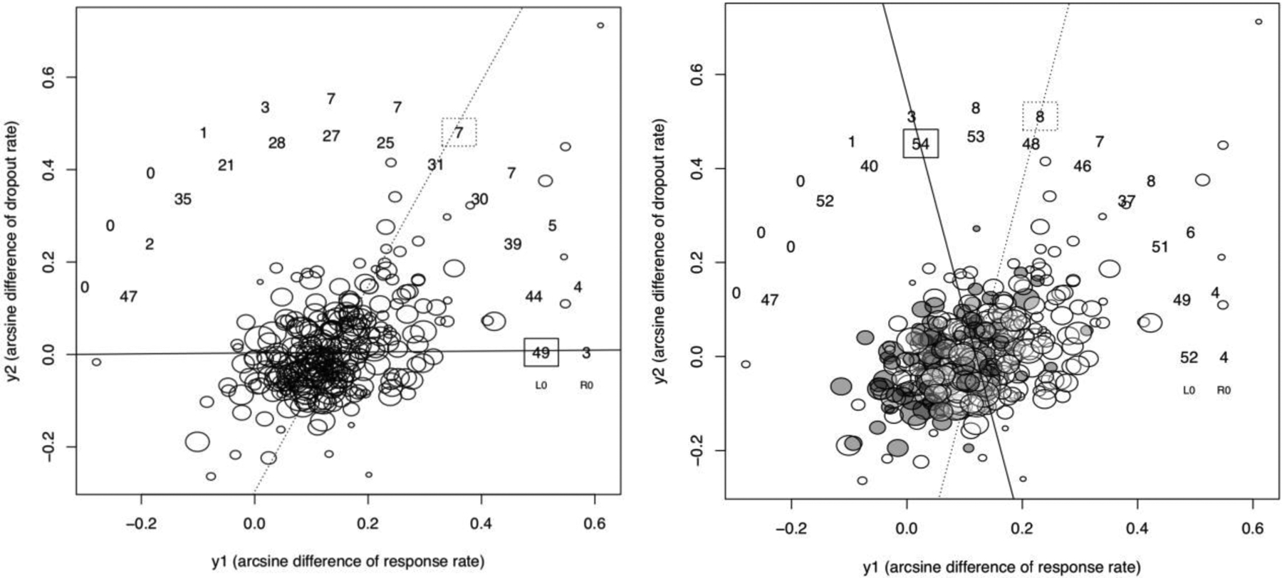
The number of trimmed studies by the proposed bivariate T&F method in the antidepressant meta-analysis of Cipriani et al³⁷. The two outcomes are the arcsine differences of response rate and dropout rate between antidepressants and placebo. The 288 published studies are presented in the galaxy plot in the left panel, while the 89 studies in the grey literature (colored) are additionally included in the right panel. The number of trimmed studies along the 12 directions of projection are shown, where the inner and outer circles are for L₀ and R₀ estimators respectively. The direction with the maximum number of trimmed studies is selected.

Table 3.

The estimated effects of efficacy (y₁) and safety (y₂) outcomes in the meta-analysis of antidepressant drugs using unadjusted, univariate and proposed bivariate T&F approaches. Larger effects favor treatment over control. Presented are the OR estimates of the two outcomes and 95% CI, or the numbers of trim and filled studies and their standard errors. The T&F method is conducted on the arcsine-difference scale and the OR is then calculated based on the filled studies.

Method	Published			Published + grey literature
	y1 (95% CI)	y2 (95% CI)	k0 (SE)	y1 (95% CI)	y2 (95% CI)	k0 (SE)
Unadjusted	1.737 (1.663, 1.813)	0.979 (0.934, 1.026)	NA	1.631 (1.571, 1.693)	1.003 (0.964, 1.043)	NA
Univariate T&F, R0	1.718 (1.645, 1.793)	1.008 (0.960, 1.059)	y1: 3 (2.8) y2: 7 (4.0)	1.602 (1.540, 1.666)	0.978 (0.933, 1.025)	y1: 4 (3.2) y2: 8 (4.2)
Bivariate T&F, R0	1.718 (1.645, 1.793)	1.008 (0.960, 1.059)	7 (4.0)	1.614 (1.552, 1.679)	0.984 (0.944, 1.025)	8 (4.2)
Univariate T&F, L0	1.557 (1.486, 1.632)	0.959 (0.915, 1.005)	y1: 49 (11.1) y2: 27 (10.8)	1.539 (1.485, 1.594)	0.909 (0.871, 0.949)	y1: 52 (12.6) y2: 53 (12.6)
Bivariate T&F, L0	1.565 (1.493, 1.641)	0.959 (0.915, 1.005)	49 (11.1)	1.576 (1.519, 1.636)	0.912 (0.874, 0.952)	54 (12.6)

In the left panel of Figure 4, the bivariate T&F using L₀ estimator trims 49 studies on the right along the horizontal direction, which identifies more trimmed studies than other directions. This selected direction indicates that the studies are missing primarily due to insufficient evidence of efficacy. Meanwhile, using R₀ estimator, only 7 studies are trimmed on the top right corner along several directions with tied number of trimmed studies. The discrepancy between the two estimators is because the missing mechanism assumption of T&F is not strictly satisfied in this real-world example, and thus the R₀ estimator can only trim those studies with extreme outcome values²⁰. Nevertheless, T&F using the R₀ estimator shows that some studies are missing with insufficient evidence of both efficacy and safety. The bias correction for both outcomes is quantified in Table 3, where the estimates of five approaches are shown. Specifically, compared to the unadjusted published only (OR = 1.737, 0.979 for efficacy and safety respectively), adding the grey literature updates the estimates (ORs = 1.631, 1.003) towards the corrected estimates using published only (bivariate T&F L₀, ORs = 1.565, 0.959). This confirmed that the grey literature has completed many of the missing studies. However, there is no guarantee that the search of grey literature³⁷ is exhaustive; hence applying the bivariate T&F to the published + grey literature still obtains some correction, i.e. ORs = 1.576, 0.912, which is consistent with the ORs after correcting published only. This imperfection of grey literature can also be seen from the right panel of Figure 4, where T&F with the R₀ estimator using published and grey literature studies obtains a similar number of trimmed studies along a similar direction as that of using published studies only, indicating that the grey literature likely does not contain the missing studies with extreme values of both outcomes.

5. Discussion

We proposed a bivariate T&F procedure as a sensitivity analysis tool for bivariate meta-analysis to account for potential PB. This bivariate T&F method is based on the symmetry of the galaxy plot, which is an extension of the funnel plot for bivariate meta-analysis. In the bivariate situation, the studies may be suppressed due to their smaller (or larger) values of the weighted sum of the two outcomes, leading to the asymmetry of the galaxy plot along a certain direction. By trimming and filling the studies that are projected onto a sequence of directions, the method can detect a potential direction along which studies are most likely to be suppressed along. When PB is due to the suppression of studies that is dependent on more than one outcome, the method can potentially achieve a better bias reduction than the univariate T&F method.

The proposed bivariate T&F method is a useful tool for exploring and correcting for PB in a bivariate meta-analysis. The method’s performance is demonstrated using simulation studies under various settings and a real-world meta-analysis of the efficacy and safety of antidepressant drugs. This large-scale meta-analysis example shows that studies are missing primarily due to efficacy, while some missing studies are possibly due to both efficacy and safety. The proposed method obtains consistent correction using either published only or published + grey literature studies. The proposed method can be generally applied to multiple efficacy outcomes when a unified reporting standard is not adopted. For example, in the SPRINT MIND study³⁹ of mild cognitive impairment and dementia, multiple cognitive outcomes have been collected using the Montreal Cognitive Assessment (MoCA⁴⁰), the Logical Memory form⁴¹, and the Digit Symbol Coding Test⁴². Besides these, the proposed method can also be applied to diagnostic test accuracy studies, where the bivariate sensitivity and specificity measures are often combined to a univariate measure for further meta-analysis^30,43. For example, the sensitivity and specificity can be combined as Youden’s index, diagnostic OR, Lehmann θ_L, or Doebler’s θ after proper transformation⁴³. As an alternative to the univariate approaches, the bivariate T&F method can be applied to detect asymmetry of the sensitivity and specificity along multiple directions in a transformed ROC space. Lastly, the proposed bivariate T&F method can be extended to multivariate meta-analysis using the same idea of projecting multivariate outcomes to univariate directions. As long as the candidate directions are properly chosen, the computational cost is small.

PB in bivariate meta-analysis is more complicated than in the univariate situation due to its multi-dimensional nature. The proposed method relies on the assumption that the publication is selective along a certain direction and transforms the problem into a number of univariate problems along candidate directions. Such an assumption can be investigated in practice using, e.g., the contour-enhanced funnel plot for the projected studies¹⁴. We also emphasize that galaxy (funnel) plot asymmetry does not equate PB, because the choice of outcome measures³², clinical heterogeneity, or natural boundaries could also lead to asymmetry^13,44. Specifically, when natural boundaries (e.g. Youden’s index, or biological maximum of the diagnostic odds ratio in a diagnostic test meta-analysis) exist, any studies being filled beyond the boundary need to be revoked when concluding the proposed bivariate T&F approach. We thus suggest the use of the bivariate T&F method as an exploratory and sensitivity analysis tool to investigate the evidence of PB.

Some well-known limitations of the univariate T&F method remain in the bivariate scenario. For example, the method is sensitive to outlying studies. As a result, it is recommended that both L₀ and R₀ estimators should be used^20,28,34. The suppressing direction is selected as the direction giving the most trimmed studies. Alternatively, one may choose the optimal direction by maximizing the skewness statistics²¹. In the real data example, it is possible that the missing studies are not suppressed by any straight line, thus using L₀ produces more trimmed studies than using R₀. A more essential limitation is that, when between-study heterogeneity is severe, the T&F method usually fails to identify missing studies and correct for the bias^35,45. In our simulation and real data examples, the heterogeneity is not severe (I² ≈ 42% in simulation and 38% in real data). The FE-RE T&F approach adopted in this article can alleviate this problem. The proposed bivariate T&F method mainly works for PB and may not be able to account for outcome reporting bias^25,1. This could be an interesting future research direction. Finally, the proposed bivariate T&F method can be integrated with bivariate meta-analysis models^18,2,3 to account for the impacts of publication bias. This extension is currently under investigation and will be reported in the future.

Data Availability Statement

The data of antidepressant drugs that support the findings of this study are openly available in The Lancet (Cipriani et al³⁷) at https://doi.org/10.1016/S0140-6736(17)32802-7.

References

- 1.Bai R, Liu X, Lin L, Liu Y, Kimmel SE, Chu H, & Chen Y (2021). A Bayesian Selection Model for Correcting Outcome Reporting Bias With Application to a Meta-analysis on Heart Failure Interventions (Version 1). arXiv. https://arxiv.org/abs/2110.08849 [Google Scholar]
- 2.Chen Y, Hong C, & Riley RD (2014). An alternative pseudolikelihood method for multivariate random-effects meta-analysis. Statistics in Medicine, 34(3), 361–380. https://pubmed.ncbi.nlm.nih.gov/25363629/ [DOI] [PMC free article] [PubMed] [Google Scholar]
- 3.Chen Y, Chu H, Luo S, Nie L, & Chen S (2011). Bayesian analysis on meta-analysis of case-control studies accounting for within-study correlation. Statistical Methods in Medical Research, 24(6), 836–855. https://pubmed.ncbi.nlm.nih.gov/22143403/ [DOI] [PMC free article] [PubMed] [Google Scholar]
- 4.Cook DJ, Mulrow CD, Haynes RB. Systematic reviews: synthesis of best evidence for clinical decisions. Ann Intern Med. 1997;126(5):376–380. [DOI] [PubMed] [Google Scholar]
- 5.Murad MH, Asi N, Alsawas M, Alahdab F. New evidence pyramid. BMJ Evidence-Based Med. 2016;21(4):125–127. [DOI] [PMC free article] [PubMed] [Google Scholar]
- 6.Higgins JPT, Thomas J, Chandler J, et al. Cochrane Handbook for Systematic Reviews of Interventions. John Wiley & Sons; 2019. [Google Scholar]
- 7.Begg CB, Berlin JA. Publication bias: a problem in interpreting medical data. J R Stat Soc Ser A (Statistics Soc. 1988;151(3):419–445. [Google Scholar]
- 8.Thornton A, Lee P. Publication bias in meta-analysis: its causes and consequences. J Clin Epidemiol. 2000;53(2):207–216. [DOI] [PubMed] [Google Scholar]
- 9.Copas JB, Shi JQ. A sensitivity analysis for publication bias in systematic reviews. Stat Methods Med Res. 2001;10(4):251–265. doi: 10.1177/096228020101000402 [DOI] [PubMed] [Google Scholar]
- 10.Rothstein HR, Sutton AJ, Borenstein M. Publication Bias in Meta-Analysis: Prevention, Assessment and Adjustments. John Wiley & Sons; 2006. [Google Scholar]
- 11.Terrin N, Schmid CH, Lau J. In an empirical evaluation of the funnel plot, researchers could not visually identify publication bias. J Clin Epidemiol. 2005;58(9):894–901. [DOI] [PubMed] [Google Scholar]
- 12.Light RJ, Richard J, Light R, Pillemer DB. Summing up: The Science of Reviewing Research. Harvard University Press; 1984. [Google Scholar]
- 13.Sterne JAC, Sutton AJ, Ioannidis JPA, et al. Recommendations for examining and interpreting funnel plot asymmetry in meta-analyses of randomised controlled trials. BMJ. 2011;343:d4002–d4002. doi: 10.1136/bmj.d4002 [DOI] [PubMed] [Google Scholar]
- 14.Peters JL, Sutton AJ, Jones DR, Abrams KR, Rushton L. Contour-enhanced meta-analysis funnel plots help distinguish publication bias from other causes of asymmetry. J Clin Epidemiol. 2008;61(10):991–996. [DOI] [PubMed] [Google Scholar]
- 15.Chu H, Cole SR. Bivariate meta-analysis of sensitivity and specificity with sparse data: a generalized linear mixed model approach. J Clin Epidemiol. 2006;59(12):1331. [DOI] [PubMed] [Google Scholar]
- 16.Chu H, Nie L, Chen Y, Huang Y, Sun W. Bivariate random effects models for meta-analysis of comparative studies with binary outcomes: methods for the absolute risk difference and relative risk. Stat Methods Med Res. 2012;21(6):621–633. doi: 10.1177/0962280210393712 [DOI] [PMC free article] [PubMed] [Google Scholar]
- 17.Chen Y, Liu Y, Ning J, Cormier J, Chu H. A hybrid model for combining case--control and cohort studies in systematic reviews of diagnostic tests. J R Stat Soc Ser C Appl Stat. 2015;64(3):469–489. https://rss.onlinelibrary.wiley.com/doi/abs/10.1111/rssc.12087 [DOI] [PMC free article] [PubMed] [Google Scholar]
- 18.Chen Y, Liu Y, Ning J, Nie L, Zhu H, Chu H. A composite likelihood method for bivariate meta-analysis in diagnostic systematic reviews. Stat Methods Med Res. 2017;26(2):914–930. doi: 10.1177/0962280214562146 [DOI] [PMC free article] [PubMed] [Google Scholar]
- 19.Hong C, Duan R, Zeng L, et al. Galaxy Plot: A New Visualization Tool of Bivariate Meta-Analysis Studies. Am J Epidemiol. 2020;189(8):861–869. doi: 10.1093/aje/kwz286 [DOI] [PMC free article] [PubMed] [Google Scholar]
- 20.Duval S, Tweedie R. A nonparametric “trim and fill” method of accounting for publication bias in meta-analysis. J Am Stat Assoc. 2000;95(449):89–98. [Google Scholar]
- 21.Lin L, Chu H. Quantifying publication bias in meta-analysis. Biometrics. 2018;74(3):785–794. doi: 10.1111/biom.12817 [DOI] [PMC free article] [PubMed] [Google Scholar]
- 22.Egger M, Smith GD, Schneider M, Minder C. Bias in meta-analysis detected by a simple, graphical test. Bmj. 1997;315(7109):629–634. [DOI] [PMC free article] [PubMed] [Google Scholar]
- 23.Peters JL, Sutton AJ, Jones DR, Abrams KR, Rushton L. Comparison of two methods to detect publication bias in meta-analysis. Jama. 2006;295(6):676–680. [DOI] [PubMed] [Google Scholar]
- 24.Galbraith RF. Some applications of radial plots. J Am Stat Assoc. 1994;89(428):1232–1242. [Google Scholar]
- 25.Marks-Anglin A, Chen Y. Small-study effects: current practice and challenges for future research. Stat Interface. 2020;13(4):475–484. [Google Scholar]
- 26.Lin L, Chu H, Murad MH, et al. Empirical Comparison of Publication Bias Tests in Meta-Analysis. J Gen Intern Med. 2018;33(8):1260–1267. doi: 10.1007/s11606-018-4425-7 [DOI] [PMC free article] [PubMed] [Google Scholar]
- 27.Lin L, Shi L, Chu H, Murad MH. The magnitude of small-study effects in the Cochrane Database of Systematic Reviews: an empirical study of nearly 30 000 meta-analyses. BMJ evidence-based Med. 2020;25(1):27–32. [DOI] [PMC free article] [PubMed] [Google Scholar]
- 28.Duval S, Tweedie R. Trim and fill: a simple funnel‐plot–based method of testing and adjusting for publication bias in meta‐analysis. Biometrics. 2000;56(2):455–463. [DOI] [PubMed] [Google Scholar]
- 29.Jackson D, Riley R, White IR. Multivariate meta-analysis: potential and promise. Stat Med. 2011;30(20):2481–2498. doi: 10.1002/sim.4172 [DOI] [PMC free article] [PubMed] [Google Scholar]
- 30.Bürkner P, Doebler P. Testing for publication bias in diagnostic meta‐analysis: a simulation study. Stat Med. 2014;33(18):3061–3077. [DOI] [PubMed] [Google Scholar]
- 31.Hong C, Salanti G, Morton SC, et al. Testing small study effects in multivariate meta‐analysis. Biometrics. 2020;76(4):1240–1250. [DOI] [PMC free article] [PubMed] [Google Scholar]
- 32.Rücker G, Schwarzer G, Carpenter J. Arcsine test for publication bias in meta‐analyses with binary outcomes. Stat Med. 2008;27(5):746–763. [DOI] [PubMed] [Google Scholar]
- 33.Youden WJ. Index for rating diagnostic tests. Cancer. 1950;3(1):32–35. doi: [DOI] [PubMed] [Google Scholar]
- 34.Shi L, Lin L. The trim-and-fill method for publication bias: practical guidelines and recommendations based on a large database of meta-analyses. Medicine (Baltimore). 2019;98(23). [DOI] [PMC free article] [PubMed] [Google Scholar]
- 35.Peters JL, Sutton AJ, Jones DR, Abrams KR, Rushton L. Performance of the trim and fill method in the presence of publication bias and between‐study heterogeneity. Stat Med. 2007;26(25):4544–4562. [DOI] [PubMed] [Google Scholar]
- 36.Moreno SG, Sutton AJ, Ades AE, et al. Assessment of regression-based methods to adjust for publication bias through a comprehensive simulation study. BMC Med Res Methodol. 2009;9(1):1–17. [DOI] [PMC free article] [PubMed] [Google Scholar]
- 37.Cipriani A, Furukawa TA, Salanti G, et al. Comparative Efficacy and Acceptability of 21 Antidepressant Drugs for the Acute Treatment of Adults With Major Depressive Disorder: A Systematic Review and Network Meta-Analysis. Focus (Madison). 2018;16(4):420–429. doi: 10.1176/appi.focus.16407 [DOI] [PMC free article] [PubMed] [Google Scholar]
- 38.Chaimani A, Higgins JPT, Mavridis D, Spyridonos P, Salanti G. Graphical tools for network meta-analysis in STATA. PLoS One. 2013;8(10):e76654. [DOI] [PMC free article] [PubMed] [Google Scholar]
- 39.Group SMI for the SR, Williamson JD, Pajewski NM, et al. Effect of Intensive vs Standard Blood Pressure Control on Probable Dementia: A Randomized Clinical Trial. JAMA. 2019;321(6):553–561. doi: 10.1001/jama.2018.21442 [DOI] [PMC free article] [PubMed] [Google Scholar]
- 40.Nasreddine ZS, Phillips NA, Bédirian V, et al. The Montreal Cognitive Assessment, MoCA: a brief screening tool for mild cognitive impairment. J Am Geriatr Soc. 2005;53(4):695–699. [DOI] [PubMed] [Google Scholar]
- 41.Wechsler D Wechsler adult intelligence scale--. Arch Clin Neuropsychol. Published online 1955. [Google Scholar]
- 42.Wechsler D Wechsler memory scale. Published online 1945.
- 43.Doebler P, Holling H, Bürkner P, Doebler P. Meta-analysis of diagnostic accuracy and ROC curves with covariate adjusted semiparametric mixtures. Psychometrika. 2015;33(18):1084–1104. [DOI] [PubMed] [Google Scholar]
- 44.Lau J, Ioannidis JPA, Terrin N, Schmid CH, Olkin I. The case of the misleading funnel plot. Bmj. 2006;333(7568):597–600. [DOI] [PMC free article] [PubMed] [Google Scholar]
- 45.Terrin N, Schmid CH, Lau J, Olkin I. Adjusting for publication bias in the presence of heterogeneity. Stat Med. 2003;22(13):2113–2126. [DOI] [PubMed] [Google Scholar]
Associated Data
This section collects any data citations, data availability statements, or supplementary materials included in this article.
Supplementary Materials