Exploring unsupervised feature extraction algorithms: tackling high dimensionality in small datasets

Abstract

Small datasets are common in many fields due to factors such as limited data collection opportunities or privacy concerns. These datasets often contain high-dimensional features, yet present significant challenges of dimensionality, wherein the sparsity of data in high-dimensional spaces makes it difficult to extract meaningful information and less accurate predictive models are produced. In this regard, feature extraction algorithms are important in addressing these challenges by reducing dimensionality while retaining essential information. These algorithms can be classified into supervised, unsupervised, and semi-supervised methods and categorized as linear or nonlinear. To overview this critical issue, this review focuses on unsupervised feature extraction algorithms (UFEAs) due to their ability to handle high-dimensional data without relying on labelled information. From this review, eight representative UFEAs were selected: principal component analysis, classical multidimensional scaling, Kernel PCA, isometric mapping, locally linear embedding, Laplacian Eigenmaps, independent component analysis and Autoencoders. The theoretical background of these algorithms has been presented, discussing their conceptual viewpoints, such as whether they are linear or nonlinear, manifold-based, probabilistic density function-based, or neural network-based. After classifying these algorithms using these taxonomies, we thoroughly and systematically reviewed each algorithm from the perspective of their working mechanisms, providing a detailed algorithmic explanation for each UFEA. We also explored how these mechanisms contribute to an effective reduction in dimensionality, particularly in small datasets with high dimensionality. Furthermore, we compared these algorithms in terms of transformation approach, goals, parameters, and computational complexity. Finally, we evaluated each algorithm against state-of-the-art research using various datasets to assess their accuracy, highlighting which algorithm is most appropriate for specific scenarios. Overall, this review provides insights into the strengths and weaknesses of various UFEAs, offering guidance on selecting appropriate algorithms for small high-dimensional datasets.

Introduction

In data analysis, particularly scientific data, complexity tends to increase rapidly as advances in science and technology occur^1,2. This complexity is characterized by a large number of covariates³which often pose challenges in uncovering relationships between variables. This challenge is further exacerbated by what is known as the curse of dimensionality⁴which refers to the exponential increase in difficulty as the number of dimensions increases^5,6. High-dimensional data can make traditional learning methods impractical, resulting in issues such as the generation of irrelevant information, inadequate training, overfitting, and instability in feature extraction and classification algorithms.

Despite the prevalence of large datasets, many domains have small datasets, particularly in fields such as disease diagnosis, fault detection in biology and biotechnology, short-term load forecasting, and medical and manufacturing areas^7–9. For example, small datasets are common in clinical data analysis, where rare diseases such as spinocerebellar ataxia have limited records worldwide^7,10. These small datasets often have a higher number of dimensions but fewer available samples, referred to as high-dimensional small-sample size (HDSSS) datasets or “fat” datasets¹¹ .

In this study, we focus on addressing the primary challenge of the curse of dimensionality in HDSSS datasets. It is essential to reduce the dimensionality of the data while preserving its temporal dependencies. Dimension reduction¹² techniques aim to overcome data complexity and enhance data quality by reducing the number of input variables¹³. These techniques are broadly categorized into feature selection¹³ and feature extraction¹⁴. Feature selection identifies the most informative features and eliminates less informative ones, and feature extraction, which transforms the input space into a lower-dimensional subspace while preserving relevant information¹⁵. Feature extraction, compare with feature selection methods, have the advantage of higher discriminating power and well control overfitting¹⁶and Feature extraction techniques are often more effective than feature selection in handling noisy data¹⁷.

Among the various techniques for dimension reduction, unsupervised feature extraction algorithms (UFEAs) significantly contribute to addressing the challenge of high dimensionality, particularly in the case of small datasets^15,18. Unsupervised methods can identify hidden patterns in data without relying on labeled datasets. This makes them well-suited for real-life datasets exhibiting noise, complexity, and sparsity. Consequently, this study focuses on exploring unsupervised feature extraction algorithms due to their robustness in handling such issues and their ability to handle sample sizes with relative insensitivity compared to supervised methods. UFEAs are broadly categorized into various criteria, such as linear vs. non-linear, global vs. local and convex vs. non-convex. Linear methods linearly map a high-dimensional space into a lower space, i.e., the lower dimensions are a linear combination of the original dimensions. Non-linear methods non-linearly map a high-dimensional space into a lower space. Global methods provide a representation of data points’ global structure. Local methods produce a better performance on manifolds where the “local geometry is close to Euclidean”, but the “global geometry is probably not”. Convex methods for dimensionality reduction optimize an objective function that does not contain any local optima.

To provide a comprehensive analysis of these algorithms, eight prominent unsupervised feature extraction algorithms have been selected for our survey. These algorithms include PCA, MDS (MDS refers to Classical MDS in this study), KPCA, ISOMAP, LLE, LE, ICA, and Autoencoders¹⁵. Each of these algorithms is built on distinct mathematical foundations and operates through different mechanisms, offering diverse approaches to dimensionality reduction in small datasets.

The main contributions of this study are outlined below:

• Categorize the selected UFEAs based on various criteria, such as projection-based vs. geometric-based vs. probabilistic-based methods, linear vs. non-linear approaches, and global vs. local techniques. This classification helps to understand the theoretical underpinnings and practical applications each algorithm.

• Evaluates the learning performance of these UFEAs with a focus on small sample sizes with high dimensionality. By examining factors such as time complexity, space complexity, classification performance, we comprehensively compare each algorithm’s effectiveness.

• Based on previous studies, we summarize the learning performance of each selected UFEA for small datasets with high dimensionality. This includes analyzing how well each algorithm addresses the curse of dimensionality and maintains the integrity of temporal dependencies in the data.

• Conduct an experiment to evaluate the selected UFEAs on the small dataset EGG200 dataset.

This paper is organized as follows: the “Literature review” section discusses the usefulness of UFEA knowledge, including background and categories, and introduces the policy for selecting UFEAs. Followed by the survey of the notable state-of-the-art UFEA algorithms, covering brief introductions, mathematical foundations (objective functions), advantages, disadvantages, applications, algorithm details, and parameter-setting guidelines. The “Comparison of algorithms based on methodology” section provides a summary and comparison of the selected algorithms based on their methodologies. The “Comparison of algorithms based on results” section presents a comparison of the algorithms based on the survey results. The “Comparison of algorithms based on machine learning model” section compares the algorithms based on the experiment results. The “Discussion” section highlights open research problems. The final section provides a summary of the study’s conclusions.

Literature review

UFEAs are techniques utilized to identify and utilize data patterns without the need for labeled outputs¹⁹. These algorithms are used for dimensionality reduction to transform high-dimensional data into a more manageable lower-dimensional form while retaining important information^20,21. This process is particularly significant for small datasets, as they often encounter overfitting issues when exposed to high-dimensional feature spaces. By reducing dimensionality, these algorithms effectively eliminate redundant and irrelevant features, thereby enhancing the performance of machine learning models. This review systematically categorizes these algorithms into three main sections: Projection-based algorithms, Geometric-solution algorithms, and Probabilistic-based algorithms^15,22–24. We specifically analyzed eight algorithms from these categories, specifically focusing on their suitability for small datasets²⁵. Figure 1 provides a comprehensive taxonomy of UFEAs.

Fig. 1.

Algorithms selected in this study.

Projection-based algorithms

Projection-based algorithms aim to project data into a lower-dimensional subspace while minimizing projection error²⁶. These algorithms are divided into linear and non-linear solutions.

• Linear projective solutions Linear projective solutions, such as PCA and ICA, reduce dimensionality by embedding data into a lower-dimensional subspace²². PCA works by finding the directions (principal components) that maximize the variance in the data, making it a widely used technique for feature extraction. ICA aims to find independent sources within the data, which makes it useful for tasks such as blind source separation.

• Nonlinear projective solutions: Nonlinear projective solutions, such as KPCA, address the limitations of linear methods by transforming the original space into a higher-dimensional feature space using a nonlinear function²⁷. KPCA employs the “kernel trick” to project data into a higher-dimensional space where linear separation is possible, making it effective for datasets with complex, nonlinear relationships^28,29.

Geometric-based algorithms

Geometric-solution algorithms exploit intrinsic structure of the data by analyzing its geometric properties³⁰. MDS, preserves the pairwise Euclidean distances between the data points, making it useful to visualize the similarity between the data points in lower dimensions¹⁵. Manifold-based solutions focus on nonlinear mapping and assume that the data is on a densely sampled manifold¹⁵. Techniques like ISOMAP and LLE aim to preserve the data’s local and global geometric relationships. ISOMAP preserves the geodesic distances between all pairs of data points by constructing a neighbourhood graph, making it suitable for uncovering the underlying structure of the data²³. LLE, on the other hand, focuses on preserving local properties by reconstructing each data point as a linear combination of its nearest neighbours, which helps maintain the local geometry of the data²³.

Probabilistic-based algorithms

Probabilistic algorithms use the estimation of the probability density function (PDF) to maximize the information in the output without making strong assumptions about data structure³¹. These methods are particularly useful for small datasets, where dense sampling may be challenging³². Autoencoders, a type of neural network, learn to encode the data into a latent space and then decode it back to the original space³². This process minimizes the reconstruction loss and helps to capture the most important features of the data.

Selection of algorithms. Our strategy to select dimensionality reduction algorithms in this study is based on three main criteria: (1) focusing exclusively on unsupervised feature extraction algorithms; (2) including the most representative and successful algorithms according to the literature; and (3) ensuring that the selected algorithms encompass all the groups described in Fig. 1: projective, geometric, and probabilistic estimators. We listed the categories that frequently appear in the reviewed literatures, and excluded those such as topological solutions, which have been proven to perform poorly on small datasets²². These criteria are particularly relevant for small datasets, as the algorithms chosen to demonstrate better learning performance in such contexts. Consequently, we examine the following eight UFEAs: PCA, ICA, MDS, ISOMAP, LLE, LE, KPCA, and Autoencoder. PCA and ICA are linear methods based on projection solutions. KPCA is a projection method designed to address non-linear issues. ISOMAP, LLE, and LE are methods based on manifold learning solutions, with ISOMAP utilizing global structure and LLE and LE adopting local structure approaches. Autoencoder is a non-convex method, based on probabilistic solutions, leverages neural network techniques. Table 1 presents the frequently employed notation in this paper.

Table 1.

Notations and description.

Symbols	Descriptions
d	Number of system variables;
n	Number of samples
	Number of intrinsic dimensions;
ℓ	Number of neighbors for ISOMAP, LLE, and LE
X	Input space
Y	Output space;
(.,.)	Positive kernel function that satisfies Mercer’s theorem
h	Hidden layer size in Autoencoders
I	Number of iterations

Principal component analysis

Principal Component Analysis³³ is a widely recognized and extensively cited linear projective method^15,22 often utilized as an initial step in various pattern recognition and classification problems to generate low-dimensional representations of datasets. Originating from the works of Pearson³⁴ and Hotelling³⁵ PCA aims to retain as much information from the original data as possible. This is achieved by discovering new variables, or principal components (PCs)³⁶ which are linear functions of the original dataset’s variables. These PCs maximize variance and are not correlated with each other. Identifying PCs allows the original data to be projected into a lower-dimensional subspace that retains the most critical information while reducing the number of variables^37,38. The objective function of PCA is as follows.

1

Here, is the covariance matrix of input . PCA seeks to find a direction (principal component) that maximizes the variance of the projected data in (1). The optimization problem can be solved using the decomposition of the eigenvalue of the covariance matrix cov(X)W =λM. The eigenproblem is solved for the principal eigenvalues ^13,39, here number of intrinsic dimensions .

Algorithm 1 shows the entire process of PCA, where PCA standardizes the data matrix , computes the covariance matrix , and performs eigenvalue decomposition to select the top eigenvectors. These eigenvectors form the transformation matrix, and the transformed data is obtained by . Parameter setting for involves using the explained variance threshold (e.g., 90–95%), employing a scree plot to identify the “elbow” point, applying cross-validation to optimize downstream task performance, or based on the domain knowledge (known intrinsic dimensions) of the dataset.

Algorithm 1.

PCA.

PCA has been applied to various fields, including face recognition, coin classification, audio classification, complex systems monitoring, image and speech processing, computer vision, text mining, visualization, biometrics, robotic sensor data, stock market forecasting, and hyperspectral data on cloud computing architecture^40–47. These fields often have a problem with small datasets with high dimensionality, and PCA has also been effectively used for dimensionality reduction, demonstrating robust performance in these scenarios^15,48,49.

Figure 2 demonstrates the dimensionality reduction process using PCA. The first sub-figure presents a 3D scatterplot of the high-dimensional data reduced to three principal components, illustrating the global structure of the data. The second subfigure presents the principal components in a 2D space, with arrows representing the direction and magnitude of the variance explained by each component. Finally, the third subfigure visualizes the projection of the data onto the first two principal components, clearly separating clusters corresponding to different classes. This sequential visualization highlights how PCA reduces dimensionality while preserving the maximum variance in the data.

Fig. 2.

Visualization of PCA (the swiss roll dataset from scikit-learn has been used for visualization).

Advantages of PCA

• Effective for data with linearly separable classes²¹.

• Non-iterative, making it less time-consuming and reducing over-fitting¹⁵.

• Low noise sensitivity.

• It does not assume a specific data distribution, thus reducing dataset complexity¹⁴.

Disadvantages of PCA

• Limited to linear hidden models.

• Selecting the threshold for the number of PCs to retain is challenging²³.

Classical multidimensional scaling

MDS⁵⁰ pertains to quantifying distances between points, such as geographical locations on a map. The primary objective of MDS is to maintain a measure of similarity or dissimilarity between data points within a multidimensional space⁴¹. The outcome of an MDS analysis is a spatial representation wherein the distances between points reflect the similarities of the corresponding objects, whereby similar objects are positioned in close proximity and dissimilar ones are placed further apart¹⁵. MDS attempts to visually depict the relationships among multiple objects and encompasses two variants: classical/metric and non-metric⁵¹. In this context, we specifically concentrate on classical MDS, which conserves linear relationships. The objective function of MDS can be defined as follows⁵²:

2

Here in Eq. (2), X represents data in higher dimensions, while Y represents embedded data⁵³. is observed dissimilarity between points in the original high-dimensional space, is Euclidean distance between the reduced -dimensional space. The goal is to minimize the difference between the original dissimilarities and the distances in the reduced space.

Algorithm 2 demonstrates the entire MDS procedure. MDS takes a distance matrix, double centres it, and performs Eigen decomposition to obtain the top eigenvectors. These eigenvectors are used to form the low-dimensional embedding . The parameter settings fo rk in MDS can be determined based on visualization goals or through cross-validation.

Algorithm 2.

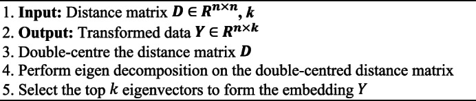
MDS.

Despite the availability of numerous dimension reduction techniques, MDS has gained popularity due to its simplicity and wide range of applications, thereby establishing itself as a standard tool among statisticians and researchers⁴¹. MDS is frequently employed for data visualization in various disciplines, including Psychology, Sociology, Anthropology, Economy, and Educational Research, and for analysing different types of data such as text, image, audio, video, time series, and structured data^15,37,54.

MDS reduces dimensionality in small, high-dimensional datasets by preserving pairwise distances between data points^15,55. It generates a configuration of points in a lower-dimensional space where the distances correspond as closely as possible to the original similarities or dissimilarities. This method is particularly useful for visualizing complex data structures.

Figure 3 illustrates the progressive results of MDS applied to high-dimensional data. The three subfigures represent the intermediate transformations at 10, 50, and 100 iterations, respectively, as MDS minimizes the stress function to embed the data into a 2D space. In the initial stages, the embedding is disordered, but as iterations progress, the structure of the data emerges more distinctly. By the final stage, clusters corresponding to different classes are well separated, emphasizing MDS’s capacity to preserve pairwise dissimilarities in lower dimensions.

Fig. 3.

Visualization of MDS (the Swiss Roll dataset from scikit-learn has been used for visualization).

Advantages of MDS

• Useful for preserving inter-point distances²⁴.

• Does not rely on strict assumptions of linearity and normality⁴¹.

• Easy to implement and produces precise solutions⁵².

• Excellent for data visualization and uncovering hidden data structures⁵².

• Requires only a matrix of pairwise distances, reducing computation and storage needs^14,53,56.

Disadvantages of MDS

• Computationally expensive¹⁵.

• Difficult to select the appropriate map dimension⁵⁴.

• Represents large distances better than small ones⁵⁴.

• Unlike PCA, MDS cannot reduce dimensions linearly.

• Sensitive to outliers and increased noise levels.

• MDS may perform poorly if interval scale conditions are unmet⁵².

Kernel principal component analysis

KPCA⁵⁷ is an extension of traditional PCA that aims to capture non-linear relationships using the kernel method²⁴. By transforming input vectors into a higher-dimensional space, KPCA has the potential to make the data more linear. Standard PCA is then carried out in this new feature space to obtain feature vectors^24,39. The kernel method is crucial in mapping complex problems from the original space to linear problems in the feature space. Commonly used kernel functions in KPCA include linear, polynomial, and Gaussian radial basis functions^37,53. Suppose is a nonlinear mapping maps the data to a higher-dimensional feature space. The objective of KPCA is to maximize the variance of the projections , along a direction in the feature space.

3

= is the covariance matrix in the feature space. In practice, directly working with in the high-dimensional feature space is computationally infeasible.

Instead, KPCA relies on the kernel trick, which avoids explicit computation in the feature space by using kernel functions. A kernel (, ) = computes the inner product in the featurespace.

The entire KPCA process is described in (Algorithm 3). KPCA computes the kernel matrix using a kernel function, centers it, and performs eigenvalue decomposition to select the top eigenvectors. The transformed data is obtained by . For setting KPCA parameters: Use a linear kernel to emulate traditional PCA behaviour, and an RBF, Poly kernels to capture non-linear data structures. Select k similar with PCA, based on the explained variance or performance in downstream tasks.

Algorithm 3.

KPCA.

The KPCA method, widely used in classification problems⁵³has proven to be effective in various domains, such as face recognition, speech recognition, novelty detection, and stock market forecasting^39,42,53. It exhibits exceptional capabilities in neuro-engineering tasks like brain disease diagnosis and EEG/ECG analysis⁵⁸surpassing PCA in feature extraction and making significant contributions to mental state assessments and clinical diagnoses^43,59,60. KPCA demonstrates its effectiveness, particularly for small datasets with intricate structures, as it reduces dimensionality while preserving non-linear patterns^15,58,61.

Figure 4 displays the results of KPCA with three different kernel functions: linear, RBF, and polynomial. Each subfigure shows the 2D projection of high-dimensional data after applying the respective kernel. The linear kernel behaves similarly to standard PCA, preserving global linear relationships. In contrast, the RBF kernel captures non-linear structures, revealing a more compact and distinct clustering of classes. The polynomial kernel strikes a balance between linear and nonlinear transformations, with moderately separated clusters. This figure highlights the flexibility of Kernel PCA in adapting to data with varying complexity.

Fig. 4.

Visualization of KPCA (the Swiss Roll dataset from scikit-learn has been used for visualization).

Advantages of KPCA

• KPCA exhibits strong performance when dealing with nonlinear data¹⁵.

• KPCA It yields a low surrogate error in complex design spaces⁵³.

• KPCA is robust in solving problems with compact sizes⁶².

Disadvantages of KPCA

• KPCA entails high computational cost and memory requirements²¹primarily due to the size of the kernel matrix³⁹.

• Kernel PCA mainly focuses on retaining large pairwise distances (even though these are now measured in feature space)^39,41.

• The process of selecting an appropriate kernel for KPCA can be challenging, as it depends on the specific problem at hand⁵³.

Isometric mapping

ISOMAP, a nonlinear unsupervised feature extraction algorithm, is regarded as one of the pioneering methods in manifold learning¹⁵. It builds on the principles of classical scaling and aims to preserve the pairwise geodesic distances between data points when projecting them onto a lower-dimensional space. The underlying assumption of ISOMAP is that data exhibit a manifold structure can be effectively represented in a reduced dimensional form through the utilization of distance maps³⁷. The objective of Isomap is to preserve the pairwise geodesic distances between data points when reducing the dimensionality of the dataset.

4

Where, is the geodesic distance between point i and j in the high-dimensional space, estimated using shortest paths on a neighborhood graph. is the geodesic distance between point i and j in the low-dimensional embedding space.

In Algorithm 4, the whole ISOMAP process is illustrated. ISOMAP constructs a neighborhood graph, computes the shortest path distances (geodesic distances), and applies MDS to the geodesic distance matrix. The result is a low-dimensional embedding . For parameters setting, select ℓ based on domain knowledge or cross-validation. Choose k by balancing explained variance and downstream performance. Use the Euclidean distance for general purposes or customize the distance metric for specific applications.

Algorithm 4.

ISOMAP.

ISOMAP has been applied to wood inspection, biomedical data visualization, head pose estimation, urban road traffic conditions, speech summarization, and facial recognition^15,39,58ISOMAP has also been applied in clinical data analysis⁶³.

ISOMAP reduces dimensionality in small, high-dimensional datasets by preserving the geodesic distances between points on a manifold (generally a nonlinear space)^15,64. It constructs a neighborhood graph, computes shortest paths, and applies MDS to find a lower-dimensional embedding. This method is effective in uncovering the intrinsic geometry of nonlinear manifolds.

Figure 5 visualizes the ISOMAP dimensionality reduction process. The three subfigures correspond to embeddings generated with an increasing number of neighbors (5, 10, and 20). With fewer neighbors, ISOMAP captures local relationships, resulting in tightly connected clusters. As the number of neighbors increases, the embeddings smooth out, revealing the global manifold structure of the data. This progression illustrates ISOMAP’s ability to balance local and global properties in manifold learning, ultimately achieving a faithful low-dimensional representation of the high-dimensional dataset.

Fig. 5.

Visualization of ISOMAP (the swiss roll dataset from scikit-learn has been used for visualization).

Advantages of ISOMAP

• Effective for nonlinear dimensionality reduction³⁹.

• Combines characteristics of PCA and MDS, providing computational efficiency, asymptotic convergence guarantees, and global optimality⁴¹.

• Suitable for learning internal flat low-dimensional manifolds³⁷.

• Robust and widely used for meaningful insights into low-dimensional structures³⁷.

Disadvantages of ISOMAP

• Topological instability, potentially building incorrect connections in the neighborhood graph^15,37,39.

• It may fail with non-convex manifolds¹⁵.

• It is not suitable for manifolds with large intrinsic curvature³⁷.

• High computational time for calculating shortest paths between sample points³⁷.

• Poor extrapolation beyond the neighborhood of training data³⁷.

• Challenges in incremental learning and performance bottlenecks^24,58.

Locally linear embedding

LLE is a technique used to learn manifolds that are close to the data and project them onto it. LLE begins by identifying the nearest neighbors of each data point and then uses a linear combination of these neighbors to represent the data point itself⁶⁵. This method preserves the linear relationships between the target point and neighbors in the low-dimensional embedding manifold. LLE is a local method, meaning the new coordinates of data points depend only on the neighborhood of that point⁵⁸. Unlike ISOMAP, which aims to preserve global properties, LLE focuses on maintaining local properties, making it less sensitive to short-circuiting because only a small number of local properties are affected if it occurs. LLE constructs the local properties of the data manifold by writing high-dimensional data points as a linear combination of their nearest neighbors and attempts to retain these reconstruction weights in the low-dimensional representation³⁹. Objective function to define LLE is given in Eq. (6).

5

Here, is the i-th point in the reduced k-dimension space. is the reconstruction weights calculated in the high-dimensional space. N(i) is the set of K nearest neighbors of x_i. The goal is to minimize to find the low-dimensional coordinates Y.

Algorithm 5 provides a detailed overview of the LLE process. LLE finds ℓ-nearest neighbors for each data point, computes the reconstruction weights , and determines the embedding coordinates Y by minimizing the reconstruction error using these weights. To set parameters for LLE, select ℓ using cross-validation, typically within the range of 5–20. Generally, choose k based on cross-validation or domain knowledge.

Algorithm 5.

LLE.

LLE has been applied in various academic domains, such as face recognition, remote sensing, and magnetic resonance imaging (MRI) (including functional MRI, seizure detection, hippocampus shape analysis in Alzheimer’s disease (AD), diffusion tensor imaging, breast lesion segmentation, feature fusion, and image classification)⁴¹prostate cancer detection, breast cancer, and spectroscopic analysis^66,67. In addition to its proficiency in handling image, audio, and video data, LLE has paved the way for developing linear variants that have proven instrumental in applications such as super-resolution and sound source localization³⁹. LLE reduces dimensionality by preserving local relationships within small, high-dimensional datasets^15,68.

Figure 6 shows the dimensionality reduction process using LLE. Similar to ISOMAP, the three sub-figures show embeddings with increasing numbers of neighbors (5, 10, and 20). The first subfigure highlights the preservation of local neighborhood relationships, while subsequent subfigures demonstrate a gradual integration of global relationships as more neighbors are considered. This progression underscores LLE’s strength in capturing complex non-linear structures while maintaining the local linearity of data points in lower dimensions.

Fig. 6.

Visualization of LLE (the swiss roll dataset from scikit-learn has been used for visualization).

Advantages of LLE

• Efficiently handles nonlinear data and sparse matrices, requiring less computational time and space compared to other FE techniques¹⁵.

• Popular for managing large, high-dimensional datasets and finding embeddings non-iteratively⁴¹.

• Optimized to avoid local minima, maintains local geometry in embedded space, and features a single global coordinate system³⁷.

• Works best for unfolding single continuous low-dimensional manifolds and is less sensitive to short-circuiting than ISOMAP, effectively embedding non-convex manifolds³⁹.

Disadvantages of LLE

• High memory consumption and sensitivity to noise¹⁵.

• Inability to handle novel data and ill-conditioned eigenproblems⁴¹.

• Assume that data reside in a continuous manifold, which is not ideal for multi-class classification problems⁴¹.

• Sensitive to parameter variations (intrinsic dimensionality d, number of nearest neighbors k, and regularization parameter α. Incorrect settings can lead to noise amplification or loss of global properties⁶⁹.

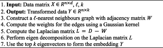
Laplacian eigenmaps

Laplacian Eigenmaps is an unsupervised nonlinear FEA aimed at finding low-dimensional representations by preserving local properties of a manifold^15,24. LE generates a neighborhood graph where each data point is connected to its nearest neighbors, with edges weighted using the Gaussian kernel function³⁹. This method finds a low-dimensional representation by preserving the local properties of the manifold. The idea is that a manifold approximated by a connected, undirected graph can map its vertices to a Euclidean subspace R^d, maintaining locality so that neighboring points remain close after mapping⁶⁹. Given a dataset X, the objective of LE is to map the data points to a lower-dimensional space Y such that the nearby points in the original space remain nearby in the embedding. This is achieved by solving the following optimization problem:

6

Where, Y is the low-dimensional embedding is the weight between day point x_i and x_j The variance (σ) specifies the Gaussian’s effect on the adjacency matrix (W). To reduce the dimensionality from X to Y, LE aims to minimize the cost function defined in (6).

The steps of LE are fully depicted in Algorithm 6. LE constructs a neighborhood graph with an adjacency matrix W, computes edge weights using a Gaussian kernel, and forms the Laplacian matrix L. Eigen decomposition on L provides the top k eigenvectors used to generate the embedding Y. To set parameters for LE, similar with LLE, select ℓ using cross-validation, typically within the range of 5–20, and choose k based on cross-validation or domain knowledge.

Algorithm 6.

LE.

LE has been applied to face recognition, functional magnetic resonance data analysis, and spectral clustering. Spectral clustering uses the coordinates obtained from LE for clustering based on their signs³⁹. LE has also been applied in clinical analysis, including pediatric cardiology diagnostics, breast cancer diagnosis, and Alzheimer’s disease diagnosis^70–72.

LE aims to preserve the local properties of a manifold within small, high-dimensional datasets^15,73.

Figure 7 shows the embedding process of Laplacian Eigenmaps for three stages with increasing neighborhood sizes (5, 10, and 20). The first sub-figure illustrates the highly localized embedding with small neighborhood connections, preserving immediate relationships. As the size of the neighborhood increases, the embedding evolves to reveal broader manifold structures, allowing better class separation. This figure highlights the flexibility of Laplacian eigenmaps in adjusting neighborhood sizes to uncover both local and global properties in the data.

Fig. 7.

Visualization of LE (the swiss roll dataset from scikit-learn has been used for visualization).

Advantages of LE

• Evaluations show that LE resembles the dual MVU problem³⁹.

Disadvantages of LE

• Shares weaknesses with LLE, such as the trivial solution problem³⁹.

• Issues with uneven data sampling, out-of-sample problems, small sample sizes, and discriminant feature extraction⁶⁹.

• Nonlinear dimensionality reduction techniques, including LE, are challenging for evaluating new test points^24,69.

Independent component analysis

ICA is an information-theory-based algorithm extending PCA by seeking independent factors instead of uncorrelated ones^24,52. The main breakthrough in the theory of ICA was the realization that the model can be made identifiable by making the unconventional assumption of the non-Gaussianity of the independent components⁷⁴. ICA assumes data is a linear mixture of independent sources and aims to find a unmixing matrix that separates the signal source vector X into statistically independent components Y^37,41. The objective function for ICA is defined below.

7

Here, X is the mixing matrix, and Y is the independent components’ basis coefficients. To obtain k dimensions from a dataset, ICA produces Y by selecting the top k independent components defined in Eq. (8)¹⁵.

8

The primary objective of ICA is to find a linear transformation W such that the resulting components in are statistically independent. Since direct independence is difficult to measure, ICA typically achieves this by maximizing non-Gaussianity of the components, using measures such as kurtosis or negentropy. This principle is motivated by the Central Limit Theorem⁷⁵which implies that a mixture of independent variables tends to be more Gaussian than the individual sources. An alternative formulation of ICA involves minimizing the mutual information among components, another valid criterion for statistical independence.

Algorithm 7 presents the comprehensive process of ICA. ICA centers and whitens the data, initializing the unmixing matrix W and iteratively updating it using a fixed-point algorithm until convergence. The independent components Y are obtained by . Set parameters k based on domain knowledge for example the meaningful independent signals or cross-validation. Use a small tolerance value and increase the number of iterations if convergence issues occur.

Algorithm 7.

ICA.

Compared to PCA, which identifies orthogonal directions that maximize variance and assumes Gaussian-distributed data, ICA goes a step further by identifying statistically independent components, making it particularly effective for blind source separation and other tasks involving non-Gaussian signals.

ICA is used for separating mixed signals, source-channel separation, recognition of speech, functional MRI, Bayesian detection, data analysis, compression, localization of sources, microarray data reduction, and hybrid search techniques such as ICA for informative gene selection^{15,28,37,53,76}.

ICA was also applied in biomedical signals analysis and imaging brain dynamics analysis^77,78. ICA reduces dimensionality by finding independent components within small, high-dimensional datasets. It separates mixed signals into statistically independent sources and selects the most informative components^15,79,80.

Figure 8 presents the results of the ICA, where the high-dimensional data is decomposed into independent components. Scatterplots show the projection of the data onto the first two independent components. The separation of clusters indicates the ability of ICA to identify statistically independent features within the data. This figure highlights ICA’s effectiveness in uncovering latent factors, making it valuable for applications like signal separation and feature extraction.

Fig. 8.

Visualization of ICA (the swiss roll dataset from scikit-learn has been used for visualization).

Advantages of ICA

• Handles large, multidimensional datasets²⁸.

• Provides more meaningful components compared to PCA⁴¹.

• Reduces overfitting risk and allows for data reconstruction in the original space⁴¹.

• Effective for separating superimposed signals⁵².

Disadvantages of ICA

• High computational complexity²⁸.

• No clear guide for ranking ICA-generated ICs⁶².

• Stochastic nature and issues with gradient-descent-based optimization methods⁴¹.

• Complications due to the curse of dimensionality in high-dimensional signal space⁴¹.

Autoencoders

Autoencoders are a class of dimensionality reduction methodologies implemented utilizing artificial neural networks^81,82. The principal objective of an autoencoder is to compress data of high dimensionality into a latent representation of lower dimensionality. This is accomplished through an encoder that maps the input data onto the latent layer, a bottleneck layer that embodies the compressed data, and a decoder that reconstructs the initial data. By minimizing the dissimilarity between the input and reconstructed output, the network can identify and retain the most significant features while discarding those of lesser importance^38,58. Given a dataset X the autoencoder maps each input x_i to a compressed representation z_i (encoding step) and reconstructs from z_i (decoding step).

The objective function is typically:

9

Where, is a loss function that measures the reconstruction error for each data point. Common choices for can be mean squared error (MSE) or binary cross-entropy (bce).

The entire autoencoder procedure is shown in Algorithm 8. Autoencoder initializes the parameters of the encoder and decoder networks, such as the hidden layer size in Autoencoders h and number of iterations I, then, defines the encoder function and the decoder function . is Neural network parameterized by . is Neural network parameterized by . And then set iterates to minimize the loss function using gradient descent. After convergence, the reconstructed data is output. For setting the parameters, design the number of neurons in the bottleneck layer based on domain knowledge or by cross-validation. Use Rectified Linear Unit(ReLU) activation for most cases but consider Sigmoid for normalized inputs⁸³.

Algorithm 8.

Autoencoder.

Autoencoders and its recent variants⁸⁴ have been well applied to classification tasks, missing data imputation, image/video classification, clustering, and creating surrogate climate models^{39,42,53,58,85}. Autoencoders have also been applied for discovering patient phenotypes, diagnosing COVID-19, and missing data imputation^86–88.1 Autoencoders reduce dimensionality by compressing data through a neural network architecture designed for reconstruction. They learn a lower-dimensional latent representation by minimizing the difference between the input and reconstructed output. Autoencoders are suitable for high-dimensional datasets, automatically identifying and retaining essential features^48,89.

Figure 9 visualizes the dimensionality reduction process using auto-encoders. The first sub-figure shows the embedding produced by a shallow autoencoder with one hidden layer that captures linear relationships. The second sub-figure demonstrates the results of a deep autoencoder with multiple hidden layers, capturing more complex nonlinear structures. The third sub-figure extends the embedding to 3D for deeper visualization of the latent space. This figure showcases Autoencoders’ versatility in learning hierarchical features and their capability to reconstruct data efficiently in a lower-dimensional representation.

Fig. 9.

Visualization of Autoencoders (the Swiss Roll dataset from scikit-learn has been used for visualization).

Advantages of autoencoder

• Automatically learn from data and are highly parallelizable⁵⁸.

• Effective for processing audio and image data⁵⁶.

• Capable of feature extraction, data generation, and denoising without assuming data distribution⁵⁶.

Disadvantages of autoencoder

• The primary drawback of autoencoders lies in the potential tediousness of their training process³⁹.

• Suitable only for datasets with reasonable dimensionality³⁹.

• Lack of interpretability and dependency on high-quality, large-scale training data⁵⁸.

Comparison of algorithms based on methodology

After providing a detailed analysis of eight unsupervised dimensionality reduction algorithms and their respective advantages and disadvantages, along with the algorithm procedure for each of the UFEAs, we have summarized the overview for each of the algorithms in this section to guide future researchers to elect the appropriate algorithm for their research problem. we have discussed the methodological differences and summaries between each algorithm in this section. Table 2 presents a comprehensive overview of taxonomy, transformation techniques, goals, parameters, and computational complexities.

Table 2.

Summarization of uefas.

Algorithm	Categorization	Taxonomy	Transformation	Goal	Parameter	Complexity
						Time	Space
PCA	Linear/Global/Convex	Projective based	Pure eigen-decomposition, linear transformation	Maximize variance	K
MDS	Linear/Global/Convex	Geometry-based(Distance)	Uses Euclidean pairwise distances; linear embedding	Preserve Euclidean pairwise distances	K	(	(
KPCA	Nonlinear/global/convex	Projective based	Kernel mapping introduces nonlinearity, but the optimization remains convex	Linearly separate data	k,		(
ISOMAP	Nonlinear/global/convex	Geometry-based (Manifold-based)	Manifold learning via geodesics (nonlinear), global structure	preserve geodesic pairwise distances	k, ℓ		(
LLE	Nonlinear/local/convex	Geometry-based (Manifold-based)	Local weights for neighbors; nonlinear manifold; convex optimization	preserve local properties	k, ℓ
LE	Nonlinear/Local/ Convex	Geometry-based (Manifold-based)	Spectral method; nonlinear but convex formulation	preserve local distances	k, ℓ	)
ICA	Linear/Local/ Convex	Projective based	Linear mixing/unmixing; iterative convex updates	maximize statistical independence	K
Autoencoder	Nonlinear/global/non-convex	Probability-based(Neural-network-based)	Neural networks introduce non-convex loss surface	minimize the distance function	K	(dnh + I)

PCA is a linear, global, and convex method that utilizes eigen decomposition to transform data. The primary objective of PCA is to optimize variance by projecting the data onto a set of orthogonal components. This method is particularly effective in identifying the most significant patterns within the data while simultaneously reducing dimensionality. The key parameter for PCA is the determination of the number of components to retain. Moreover, it exhibits a time complexity of (d²n + d³), making it relatively resource-intensive for extremely large datasets yet efficient for small to moderate-size datasets.

MDS is a linear, global, and convex method that aims to preserve Euclidean pairwise distances between data points. It achieves this by constructing a dissimilarity matrix and representing the data in a lower-dimensional space while accurately maintaining these distances. The parameters to consider are the number of components and the required iterations for convergence. MDS has a time complexity of (n³), making it suitable for datasets, where preserving pairwise distances are crucial. However, it may be computationally intensive for huge datasets.

KPCA expands on the concept of PCA by utilizing kernel functions to map data points into a higher-dimensional space, thus capturing non-linear relationships. It is a projective-based, non-linear, global, and convex method that subsequently applies PCA in this newly transformed space to identify principal components. The primary parameters to consider are the number of components and the selection of the kernel function. Notably, KPCA exhibits a computational complexity of (n³+, rendering it highly effective in uncovering intricate, non-linear patterns within datasets of high dimensionality.

ISOMAP is a geometry-based (manifold-based), non-linear, global, and convex method that focuses on preserving geodesic pairwise distances. It achieves this by constructing a neighborhood graph and calculating the shortest paths between all pairs of points to capture the intrinsic geometry of the data manifold. The primary parameter is the number of neighbors () used to build the neighborhood graph. ISOMAP’s computational complexity is (dlog()nlog(n)) + (n² ( +log(n)))+ (kn²), indicating significant computational demands. However, it is robust in uncovering non-linear manifold structures in high- dimensional data.

LLE is a geometry-based (manifold-based), non-linear, local, and convex method that preserves local properties by representing each data point as a linear combination of its nearest neighbors. The primary step involves constructing a neighborhood graph with reconstruction weights. LLE focuses on maintaining the local structure of the data manifold, making it effective in capturing local linear patterns. The primary parameter to consider is the number of neighbors (), and the computational complexity is (dlog()nlog(n)) +(dn ³) +(kn²). While this complexity can be high, it is manageable for small datasets.

LE is a manifold-based method aiming to preserve non-linear and convex local distances. LE constructs a neighborhood graph and updates edge weights using a Gaussian kernel function. The main objective is to map the data to a lower-dimensional space while retaining the local relationships. The key parameters are the number of neighbors () and the variance parameter (σ). The computational complexity is (dlog()nlog(n)) +(dn ³) + (kn²), which makes it well-suited for datasets where preserving local structures is important.

ICA is a linear and convex method that separates mixed signals into statistically independent components. ICA maximizes the statistical independence of the components, making it effective for feature extraction and signal separation. The main parameters are the number of components, iterations, and tolerance. The computational complexity is (2dI(d + 1) n), which reflects its efficiency in separating independent sources within high-dimensional data.

Autoencoders are non-convex neural network-based methods that map input data to a lower-dimensional latent space and reconstruct the original data by minimizing a reconstruction loss, typically a distance function such as mean squared error. Their computational complexity is (dnh + I), where d is the number of input variables, n is the number of samples, h is the hidden layer size, and I is the number of training iterations. The network architecture, including the number of layers, hidden units, activation functions, and training epochs, directly influences both the learning capacity and the computational cost. For example, deeper networks with nonlinear activations such as ReLU or GELU may provide better generalization but require significantly more resources during both training and inference. As a result, autoencoders are better suited for applications with ample computational resources and where the use of deep learning techniques provides meaningful performance advantages over linear or shallow alternatives.

Upon comparing these algorithms, it becomes apparent that each method possesses distinct strengths and limitations that cater to different data types and specific analytical objectives. PCA and KPCA excel in analyzing linear and non-linear data structures, respectively, with the latter extending the capabilities of PCA through kernel mapping. MDS, ISOMAP, LLE, and LE primarily focus on preserving various types of distances, either globally or locally, with ISOMAP and LLE particularly adept at manifold learning. Autoencoders offer a robust approach to dimensionality reduction based on neural networks, albeit requiring substantial computational resources. ICA stands out due to its ability to handle mixed signals and accentuate statistical independence, making it well-suited for applications involving feature extraction and signal separation. Each algorithm’s effectiveness depends on the dataset’s specific characteristics, the availability of computational resources, and the precise objectives of the dimensionality reduction task.

Comparison of algorithms based on results

Table 3 highlights the diverse performance of unsupervised feature extraction algorithms across various datasets. To provide a more nuanced understanding of these results, we analyze the interplay between algorithmic characteristics and dataset properties.

Table 3.

Result analysis of uefas.

Algorithm	Ref	Dataset		Model	Accuracy
		Name	Original instances/dimension		Fully selected feature set	UFEA selected feature set
PCA	Haq et al.48	Breast cancer wisconsin (original) WBC dataset	699	Relief-support vector machine	Test accuracy 89%	Test accuracy 98.33%
	Anowar et al.15	ECG200 dataset	96	Kernel support vector machine	F1 score: 89.66%	F1 score: 92.05%
	Sudharsan et al.49	Alzheimer’s disease neuroimaging initiative (ADNI)	240	Import vector machine	Test accuracy 79.03%	Test accuracy 81.03%
	Li, D. C et al.90	Pima100 dataset	8	Support vector machine	–	Test accuracy 70.81%
	Li, D. C et al.90	Breast100 dataset	30	Support vector machine		Test accuracy 93.21%
MDS	Rehman et al.55	MIPS	109	Bagging	–	Recall 54%
	Anowar et al.15	ECG200 dataset	96	Kernel support vector machine	F1 score: 89.66%	F1 score: 91.68%
KPCA	Dinesh et al.61	Pima Indians diabetes dataset	8	Support vector machine	Test accuracy 98.23%	Test accuracy 99.53%
	Anowar et al.15	ECG200 dataset	96	Kernel support vector machine	F1 score: 89.66%	F1 score: 93.03%
	Li, D. C et al.90	Pima100 dataset	8	Support vector machine	–	Test accuracy 72.74%
	Li, D. C et al.90	Breast100 dataset	30	Support vector machine	–	Test accuracy 94.85%
ISOMAP	Li et al.64	dbAMEPNI dataset	108	XGBoost	–	Test accuracy 76.8%
	Anowar et al.15	ECG200 dataset	96	Kernel support vector machine	F1 score: 89.66%	F1 score: 90.22%
LLE	Chao et al.68	Microarray dataset	72	Support vector machine	–	Test accuracy 95%
	Anowar et al.15	ECG200 dataset	96	Kernel support vector machine	F1 score: 89.66%	F1 score: 91.63%
LE	Srivastava et al.73	UCI-HAR dataset	30	XGBoost	Test accuracy 93.8%	Test accuracy 95.97%
	Anowar et al.15	ECG200 dataset	96	Kernel support vector machine	F1 score: 89.66%	F1 score: 91.81%
ICA	Aziz et al.80	Lung cancer II dataset	65	Artificial neural networks	Test accuracy 81.78%	Test accuracy 94.78%
	Musheer et al.79	Leukemia2 dataset	30	Naıive bayes	Test accuracy 87.21%	Test accuracy 97.12%
	Anowar et al.15	ECG200 dataset	96	Kernel support vector machine	F1 score: 89.66%	F1 score: 92.71%
Autoencoder	Haq et al.48	Breast cancer wisconsin (original) WBC dataset	699	Relief-support vector machine	Test accuracy 97.22%	Test accuracy 99.01%
	Xu et al.89	Genomics of drug sensitivity in cancer (GDSC)	139	Random Forest	–	Test accuracy 65.35%

PCA generally performs well on datasets with linear feature correlations and high dimensionality, such as the WBC and ECG200 datasets. These datasets benefit from PCA’s ability to project data into directions of maximum variance. For instance, in the ECG200 dataset (96 instances, 96 features), PCA improves the F1 Score from 89.66 to 92.05%, likely because the dominant linear features are preserved. However, PCA may not fully capture the underlying structure in datasets with more complex, nonlinear relationships, hence the relatively modest gain in the ADNI dataset.

MDS is effective at preserving global distance structures but does not inherently capture class separability. Its mixed performance reflects this: it improves the F1 Score in ECG200 with Kernel SVM (91.68%), suggesting global structures align with class boundaries. However, it performs poorly on MIPS (Recall: 54%), which likely suffers from class overlap or local noise that MDS cannot resolve due to its global nature. KPCA is specifically powerful in datasets with nonlinear patterns, as it maps data into higher-dimensional feature spaces using kernel functions. Its superior performance on the Pima Indians Diabetes dataset (accuracy increases from 98.23 to 99.53%) and ECG200 (F1 Score increases to 93.03%) indicates that these datasets have underlying nonlinear structures that KPCA can exploit, unlike PCA or MDS.

ISOMAP maintains global geodesic distances, making it suitable for manifolds where class structure follows curved manifolds. The moderate improvement in ECG200 and dbAMEPNI (up to 90.22 and 76.8%, respectively) suggests ISOMAP can help when global data geometry reflects class structure. However, its reliance on accurate nearest-neighbor graphs can make it sensitive to noise or sparsity, limiting its benefits on small or noisy datasets.

LLE focuses on local neighborhood preservation, making it effective where local structures encode class information. Its notable gain in Microarray and ECG200 datasets (up to 95% and 91.63%, respectively) reflects this. Microarray datasets often exhibit high sparsity with complex clusters, where local topology is more informative than global structure.

LE also preserves local similarity and is graph-based, like LLE. Its consistent improvements (e.g., 95.97% in UCI-HAR) show that LE handles both nonlinear manifolds and large feature sets effectively. Its robustness in the ECG200 dataset further confirms its strength in handling compact, structured data with well-defined local neighborhoods.

ICA excels when the features are statistically independent and non-Gaussian. In bioinformatics datasets like Leukemia2 and Lung Cancer II, which typically exhibit non-Gaussian distributions, ICA achieves large performance gains (up to 97.12%). Its performance on ECG200 also supports its value in separating independent signal sources.

Autoencoders are data-driven nonlinear models capable of learning complex feature hierarchies. Their improvements in WBC and GDSC (from 97.22 to 99.01 and 65.35%, respectively) show strength in feature compression and denoising, particularly for structured or large-scale data. Their flexibility allows adaptation to various data types, but training may require more instances to avoid overfitting.

Fig. 10.

A guide to choose the appropriate algorithms: PCA, MDS, KPCA, LLE, LE, isomap, ICA, and autoencoder.

Comparison of algorithms based on machine learning model

Experimental setup

To evaluate the performance of eight unsupervised dimensionality reduction algorithms, we use the ECG200 dataset⁹¹ that comes with 200 samples and 96 real-valued features. Among them, 133 samples are labeled as Normal and 67 as Abnormal. We used Python 3.12.2 for implementation and conducted experiments on a machine with an Apple M1 Pro, total number of cores is 10, 32GB RAM and MaC OS Sonoma 14.1.2. The dataset was split into 70% training and 30% testing sets for all experiments.

UFEAs selection and setup

We selected eight representative unsupervised feature extraction algorithms (UFEAs): PCA, Classical MDS, KPCA, Isomap, LLE, LE, FastICA, and Autoencoder. These methods span linear and nonlinear families with distinct mathematical principles.

To determine the dimensionality k, we varied it from 2 to 96 and selected the first dimension that achieved an F1 score greater than 90%. This resulted in k = 6 being used uniformly across all methods for fair comparison. For graph-based methods (Isomap, LLE, LE), we varied the number of neighbors ℓ∈ [2,6] and selected the best value based on classification accuracy. For KPCA, a polynomial kernel was used. For LE, the heat kernel width σ was estimated using the Silverman heuristic. The autoencoder was trained using a shallow architecture with one hidden layer and ReLU activation, optimized using the Adam optimizer. Table 4 summarizes the parameter settings.

Table 4.

Parameters setting for experiments.

Algorithm	Parameters setting
PCA	k: 2 to 96
MDS	k: 2 to 96
KPCA	k: 2 to 96,:Poly
Isomap	k: 2 to 96, ℓ:2 to 6
LLE	k: 2 to 96, ℓ:2 to 6
LE	k: 2 to 96, ℓ:2 to 6
FastICA	k: 2 to 96
Autoencoder	k: 2 to 96

Classification results

Table 5 presents the classification performance of eight unsupervised feature extraction algorithms on the ECG200 dataset using a support vector machine (SVM) classifier. Among these methods, LE achieved the highest accuracy (93.3%), precision (93.6%), sensitivity (97.8%), and F1 score (95.7%). LE also had the lowest false negative rate (2.2%) and false discovery rate (6.7%). In terms of runtime, LE completed in just 0.015 s, significantly faster than the autoencoder, which required 1.853 s. This result may initially seem counterintuitive since the theoretical time complexity of LE is higher than that of PCA. The complexity of LE is given by where is the number of features and is the number of data samples. In contrast, PCA has a lower complexity is Given that and in our experiment, LE’s theoretical complexity is indeed higher. However, several practical considerations explain the observed behavior. First, while asymptotic complexities describe the scaling behavior, real-world runtimes also depend on constant factors, implementation efficiency, and algorithmic overhead. LE involves eigen decomposition of a sparse Laplacian matrix, which is computationally efficient for small and is well-optimized in most numerical libraries. Second, autoencoders introduce considerable runtime overhead due to their iterative training process. Although their computational complexity can be expressed as where is the number of hidden units and denotes the number of training iterations, neural networks require multiple forward and backward passes. These operations are repeated over many epochs, contributing significantly to the overall runtime. Third, the nature of computation in LE and autoencoders is different. LE computes pairwise similarities and performs a one-time eigen decomposition. In contrast, autoencoders involve training with gradient descent, which can be computationally expensive even for small datasets due to multiple layers and parameter tuning. Finally, for small datasets like ECG200 , the term in LE does not result in significant runtime growth. This allows LE to remain both computationally efficient and highly accurate on such data sizes. LE has a higher theoretical time complexity than PCA and appears lower than that of autoencoders in practical applications, its runtime remains short due to efficient computation steps and lack of iterative training. The observed runtime differences in Table 5 are consistent with theoretical expectations when considering the dataset size, nature of operations, and implementation overheads.

Table 5.

Comparison based on support vector machine model.

Dim (k)	Accuracy	Precision	Sensitivity	False positive rate	False negative rate	False discovery rate	Negative predictive	Running time(s)	F1 score	Rank	Algorithm
6	0.783	0.864	0.844	0.4	0.156	0.133	0.563	0.004	0.854	5	PCA
6	0.818	0.908	0.844	0.26	0.156	0.087	0.611	0.282	0.875	2	MDS
6	0.817	0.886	0.867	0.333	0.133	0.111	0.625	0.172	0.876	3	KPCA
6	0.767	0.844	0.844	0.467	0.156	0.156	0.533	0.019	0.844	7	Isomap
6	0.8	0.851	0.889	0.467	0.111	0.156	0.615	0.014	0.87	4	LLE
6	0.933	0.936	0.978	0.2	0.022	0.067	0.923	0.015	0.957	1	LE
6	0.75	0.841	0.822	0.467	0.178	0.156	0.5	0.005	0.831	8	FastICA
6	0.778	0.84	0.873	0.507	0.127	0.169	0.56	1.853	0.855	6	Autoencoder

Discussion

Recent improvements in feature extraction are largely driven by deep learning models such as Convolutional Neural Networks (CNNs), autoencoders, and transformers. These architectures are widely used to extract hierarchical, task-specific features, particularly in domains like image, text, and audio analysis, offering significant advancements in performance and automation. However, several unresolved issues persist. One major concern is the lack of interpretability—many deep models, especially autoencoders, produce abstract features that are difficult to understand, limiting their applicability in sensitive fields such as healthcare. Additionally, these high-capacity models are vulnerable to overfitting, especially when trained on small or imbalanced datasets, where they may extract spurious patterns that do not generalize well. Addressing these challenges is essential for more reliable and trustworthy deployment of feature extraction methods.

This review has provided a comprehensive overview of UFEAs for small, high-dimensional datasets. By examining eight representative UFEAs—PCA, MDS, KPCA, ISOMAP, LLE, LE, ICA, and Autoencoders—we have highlighted their theoretical foundations and categorized them based on their linearity, locality, and underlying principles. Our comparative analysis focused on these algorithms’ accuracy and computational efficiency, revealing their respective strengths and weaknesses. This review emphasizes the importance of selecting appropriate UFEAs to address the challenges posed by high-dimensional data, particularly in scenarios where labelled information is scarce. The insights gained from this survey can guide researchers in choosing suitable dimensionality reduction techniques, ultimately enhancing the performance of predictive models on small datasets.

UFEAs applications on small datasets faces challenges such as overfitting, poor generalization, and unstable results. Advanced methods like multiple imputations and robust models minimize overfitting, ensuring reliable analysis while preserving data integrity and underlying relationships. Data augmentation, transfer learning, and semi-supervised approaches improve generalization. Stability can be enhanced with ensemble methods or pre-trained models. These strategies collectively enhance performance on small datasets.

Emerging trends in unsupervised feature extraction for small datasets are increasingly focused on utilizing self-supervised learning, transfer learning from large-scale datasets, and integrating domain-specific priors to enhance performance. These advanced techniques offer significant promise in overcoming the challenges posed by limited data, enabling models to capture more meaningful patterns and representations. Future research should focus on applying these reliable Unsupervised Feature Extraction Algorithms across datasets of varying sizes, rigorously evaluating their feature robustness, interpretability, and scalability. By developing algorithms that can effectively handle high-dimensional data with limited samples, future research will address the way for broader, more impactful applications in complex domains.

Conclusion

This survey has provided a comprehensive overview of unsupervised feature extraction algorithms (UFEAs) for small, high-dimensional datasets. By examining eight representative UFEAs—PCA, MDS, KPCA, ISOMAP, LLE, LE, ICA, and Autoencoders—we have highlighted their theoretical foundations and categorized them based on their linearity, locality, and underlying principles. Our comparative analysis focused on these algorithms’ accuracy and computational efficiency, revealing their respective strengths and weaknesses. This survey emphasizes the importance of selecting appropriate UFEAs to address the challenges posed by high-dimensional data, particularly in scenarios where labeled information is scarce. The insights gained from this survey can guide researchers in choosing suitable dimensionality reduction techniques, ultimately enhancing the performance of predictive models on small datasets.

Author contributions

H.N. conceived the study. H.N. drafted the manuscript. H.N. designed the experiments and wrote the programs. H.N. and S.A. analyzed the results. G.B.M., A.B.C., and K.K. helped in the analysis and discussion and gave useful comments. All authors read and approved the final manuscript.

Data availability

This study obtained research data from publicly available online repositories. https://www.timeseriesclassification.com/description.php?Dataset=ECG200 We mentioned their sources using proper citations.

Declarations

Competing interests

The authors declare no competing interests.

References

- 1.Benbya, H. et al. Complexity and information systems research in the emerging digital world. MIS Q.44 (1), 1–17 (2020). [Google Scholar]
- 2.Donoho, D. Data science at the singularity. Harvard Data Sci. Rev.6 (1) (2024).
- 3.Ma, Y. & Zhu, L. A review on dimension reduction. Int. Stat. Rev.81 (1), 134–150 (2013). [DOI] [PMC free article] [PubMed] [Google Scholar]
- 4.Bellman, R. Dynamic programming. Science153 (3731), 34–37 (1966). [DOI] [PubMed] [Google Scholar]
- 5.Tenenbaum, J. B., De Silva, V. & Langford, J. C. A global geometric framework for nonlinear dimensionality reduction. Science290 (5500), 2319–2323 (2000). [DOI] [PubMed] [Google Scholar]
- 6.Saul, L. K. & Roweis, S. T. An introduction to locally linear embedding. [DOI] [PubMed]
- 7.Handling a Small Dataset Problem in Prediction Model by employ Artificial Data Generation Approach. A Review. Journal of Physics: Conference Series; (2017).
- 8.Andonie, R. Extreme data mining: inference from small datasets. Int. J. Comput. Commun. Control. 5 (3), 280–291 (2010). [Google Scholar]
- 9.Hong, N. et al. State of the Art of machine Learning–Enabled clinical decision support in intensive care units: literature review. JMIR Med. Inf.10 (3), e28781. 10.2196/28781 (2022). [DOI] [PMC free article] [PubMed] [Google Scholar]
- 10.Taroni, J. N. et al. MultiPLIER: a transfer learning framework for transcriptomics reveals systemic features of rare disease. Cell. Syst.8 (5), 380–394 (2019). e4. [DOI] [PMC free article] [PubMed] [Google Scholar]
- 11.Friedman, J., Hastie, T. & Tibshirani, R. The Elements of Statistical Learning (Springer Series in Statistics, 2001).
- 12.Fodor, I. K. A Survey of Dimension Reduction Techniques (Lawrence Livermore National Lab., 2002).
- 13.Van Der Maaten, L., Postma, E. & Van den Herik, J. Dimensionality reduction: a comparative. J. Mach. Learn. Res.10 (66–71), 13 (2009). [Google Scholar]
- 14.Nakra, A. & Duhan, M. Feature extraction and dimensionality reduction techniques with their advantages and disadvantages for EEG-based BCI system: A review. IUP J. Comput. Sciences ;14 (1) (2020).
- 15.Anowar, F., Sadaoui, S. & Selim, B. Conceptual and empirical comparison of dimensionality reduction algorithms (PCA, KPCA, LDA, MDS, SVD, LLE, ISOMAP, LE, ICA, t-SNE). Comput. Sci. Rev.40, 100378 (2021). [Google Scholar]
- 16.Hira, Z. M. & Gillies, D. F. A review of feature selection and feature extraction methods applied on microarray data. Adv. Bioinformat. 2015 (2015). [DOI] [PMC free article] [PubMed]
- 17.A Survey of Feature Selection and Feature Extraction Techniques in Machine Learning. Science and Information Conference (IEEE, 2014).
- 18.Yan, J. et al. Effective and efficient dimensionality reduction for large-scale and streaming data preprocessing. IEEE Trans. Knowl. Data Eng.18 (3), 320–333 (2006). [Google Scholar]
- 19.Cunningham, J. P. & Ghahramani, Z. Linear dimensionality reduction: survey, insights, and generalizations. J. Mach. Learn. Res.16 (1), 2859–2900 (2015). [Google Scholar]
- 20.Sedlmair, M. et al. Dimensionality reduction in the wild: Gaps and guidance. Dept Comput Sci, Univ British Columbia, Vancouver, BC, Canada, Tech Rep TR-2012-03 (2012).
- 21.Hurtik, P., Molek, V. & Perfilieva, I. Novel dimensionality reduction approach for unsupervised learning on small datasets. Pattern Recogn.103, 107291 (2020). [Google Scholar]
- 22.Campadelli, P. et al. Intrinsic dimension estimation: relevant techniques and a benchmark framework. Math. Probl. Eng.2015 (2015).
- 23.Ceruti, C. et al. Danco: an intrinsic dimensionality estimator exploiting angle and norm concentration. Pattern Recogn.47 (8), 2569–2581 (2014). [Google Scholar]
- 24.Sorzano, C. O. S., Vargas, J. & Montano, A. P. A survey of dimensionality reduction techniques. arXiv (2014).
- 25.Silva, V. & Tenenbaum, J. Global versus local methods in nonlinear dimensionality reduction. Adv. Neural Inform. Process. Syst.15 (2002).
- 26.Camastra, F. & Staiano, A. Intrinsic dimension estimation: advances and open problems. Inf. Sci.328, 26–41 (2016). [Google Scholar]
- 27.Ghojogh, B. et al. Feature selection and feature extraction in pattern analysis: A literature review. arXiv (2019).
- 28.Saini, O. & Sharma, S. A review on dimension reduction techniques in data mining. Comput. Eng. Intell. Syst.9, 7–14 (2018). [Google Scholar]
- 29.Hoffmann, H. Kernel PCA for novelty detection. Pattern Recogn.40 (3), 863–874 (2007). [Google Scholar]
- 30.Ventura, J. et al. A novel geometric method based on conformal geometric algebra applied to the resection problem in two and three dimensions. J. Geodesy. 98 (6), 47 (2024). [Google Scholar]
- 31.Tipping, M. E. & Bishop, C. M. Probabilistic principal component analysis. J. Royal Stat. Society: Ser. B (Statistical Methodology). 61 (3), 611–622 (1999). [Google Scholar]
- 32.Baggenstoss, P. M. & Kay, S. Nonlinear dimension reduction by PDF estimation. IEEE Trans. Signal. Process. (2022).
- 33.Wold, S., Esbensen, K. & Geladi, P. Principal component analysis. Chemometr. Intell. Lab. Syst.2 (1–3), 37–52 (1987). [Google Scholar]
- 34.Pearson, K. LIII. On lines and planes of closest fit to systems of points in space. Lond. Edinb. Dublin Philosophical Magazine J. Sci.2 (11), 559–572 (1901). [Google Scholar]
- 35.Hotelling, H. Analysis of a complex of statistical variables into principal components. J. Educ. Psychol.24 (6), 417 (1933). [Google Scholar]
- 36.Jolliffe, I. T. & Cadima, J. Principal component analysis: a review and recent developments. Phil. Trans. R. Soc. A Math. Phys. Eng. Sci.374 (2065), 20150202 (2016). [DOI] [PMC free article] [PubMed]
- 37.Jia, W. et al. Feature dimensionality reduction: a review. Complex. Intell. Syst.8 (3), 2663–2693 (2022). [Google Scholar]
- 38.Bozdal, M., Ileri, K. & Ozkahraman, A. Comparative analysis of dimensionality reduction techniques for cybersecurity in the swat dataset. J. Supercomputing. 80 (1), 1059–1079 (2024). [Google Scholar]
- 39.Van Der Maaten, L., Postma, E. O. & van den Herik, H. J. Dimensionality reduction: A comparative review. J. Mach. Learn. Res.10 (66–71), 13 (2009). [Google Scholar]
- 40.Face recognition using eigenfaces. IEEE computer society conference on computer vision and pattern recognition. IEEE Computer SocietyProceedings (1991).
- 41.Nanga, S. et al. Review of dimension reduction methods. J. Data Anal. Inform. Process.9 (3), 189–231 (2021). [Google Scholar]
- 42.Rani, R. et al. Big data dimensionality reduction techniques in iot: review, applications and open research challenges. Cluster Comput.25 (6), 4027–4049 (2022). [Google Scholar]
- 43.Vaswani, N., Chi, Y. & Bouwmans, T. Rethinking PCA for modern data sets: Theory, algorithms, and applications [scanning the issue]. Proceedings of the IEEE106 (8), 1274–1276 (2018).
- 44.Huber, R. et al. Classification of coins using an eigenspace approach. Pattern Recognit. Lett.26 (1), 61–75 (2005). [Google Scholar]
- 45.Velliangiri, S. & Alagumuthukrishnan, S. A review of dimensionality reduction techniques for efficient computation. Procedia Comput. Sci.165, 104–111 (2019). [Google Scholar]
- 46.Thangavel, K. & Pethalakshmi, A. Dimensionality reduction based on rough set theory: A review. Appl. Soft Comput.9 (1), 1–12 (2009). [Google Scholar]
- 47.PCA-based multivariate anomaly detection in mobile healthcare applications. IEEE/ACM 21st International Symposium on Distributed Simulation and Real Time Applications (DS-RT) (IEEE, 2017).
- 48.Haq, A. U. et al. Detection of breast cancer through clinical data using supervised and unsupervised feature selection techniques. IEEE Access.9, 22090–22105 (2021). [Google Scholar]
- 49.Sudharsan, M. & Thailambal, G. Alzheimer’s disease prediction using machine learning techniques and principal component analysis (PCA). Materials Today: Proceedings81, 182–1 90 (2023).
- 50.Multiscale estimation of intrinsic dimensionality of data sets. 2009 AAAI Fall Symposium Series. -Torgerson WS. Multidimensional Scaling: I. Theory and Method.Psychometrika17 (4), 401 –419. (2009).
- 51.Wickelmaier, F. An introduction to MDS. Sound Qual. Res. Unit. Aalborg Univ. Denmark. 46 (5), 1–26 (2003). [Google Scholar]
- 52.Sumithra, V. & Surendran, S. A review of various linear and Non linear dimensionality reduction techniques. Int. J. Comput. Sci. Inf. Technol.6 (3), 2354–2360 (2015). [Google Scholar]
- 53.Hou, C. K. J. & Behdinan, K. Dimensionality reduction in surrogate modeling: A review of combined methods. Data Sci. Eng.7 (4), 402–427 (2022). [DOI] [PMC free article] [PubMed] [Google Scholar]
- 54.Carreira-Perpinán, M. A. A review of dimension reduction techniques. Department Comput. Sci. Univ. Sheff. Tech. Rep. CS. 96-09, 9:1–69 (1997). [Google Scholar]
- 55.ur Rehman, Z., Idris, A. & Khan, A. Multi-dimensional scaling based grouping of known complexes and intelligent protein complex detection. Comput. Biol. Chem.74, 149–156 (2018). [DOI] [PubMed] [Google Scholar]
- 56.Shetty, A. & AV, N. Performance evaluation of dimensionality reduction techniques on hyperspectral data for mineral exploration. Earth Sci. Inf.16 (1), 25–36 (2023). [Google Scholar]
- 57.Schölkopf, B., Smola, A. & Müller, K-R. Nonlinear component analysis as a kernel eigenvalue problem. Neural Comput.10 (5), 1299–1319. 10.1162/089976698300017467 (1998). [Google Scholar]
- 58.Tang, Y., Chen, D. & Li, X. Dimensionality reduction methods for brain imaging data analysis. ACM Comput. Surv. (CSUR). 54 (4), 1–36 (2021). [Google Scholar]
- 59.Dhibi, K. et al. A hybrid approach for process monitoring: improving data-driven methodologies with dataset size reduction and interval-valued representation. IEEE Sens. J.20 (17), 10228–10239 (2020). [Google Scholar]
- 60.Fezai, R. et al. Online reduced kernel principal component analysis for process monitoring. J. Process Control. 61, 1–11 (2018). [Google Scholar]
- 61.Diabetes mellitus prediction system using hybrid KPCA-GA-SVM feature selection techniques. Journal of Physics: Conference Series. (IOP Publishing, 2021).
- 62.Mulla, F. R. & Gupta, A. K. A review paper on dimensionality reduction techniques. J. Pharm. Negat. Results2022, 1263–1272.
- 63.Weng, S. et al. Mining the structural knowledge of high-dimensional medical data using isomap. Med. Biol. Eng. Comput.43, 410–412 (2005). [DOI] [PubMed] [Google Scholar]
- 64.Li, K. et al. Prediction of hot spots in protein–DNA binding interfaces based on supervised isometric feature mapping and extreme gradient boosting. BMC Bioinform.21, 1–10 (2020). [DOI] [PMC free article] [PubMed] [Google Scholar]
- 65.Huo, X., Ni, X. S. & Smith, A. K. A survey of manifold-based learning methods. Recent Adv. Data Min. Enterp. Data2007, 691–745.
- 66.Consensus-locally linear embedding (C-LLE): application to prostate cancer detection on magnetic resonance spectroscopy. Medical Image Computing and Computer-Assisted Intervention–MICCAI 2008: 11th International Conference, Proceedings, Part II 11. Visualization with Locally Linear Embedding (Springer, 2008). [DOI] [PubMed]
- 67.Ward, J. & Lumsden, S. Locally linear embedding: dimension reduction of massive Protostellar spectra. Mon. Not. R. Astron. Soc.461 (2), 2250–2256 (2016). [Google Scholar]
- 68.Feature dimension reduction for microarray data analysis using locally linear embedding. Proceedings of the 3rd Asia-Pacific Bioinformatics Conference. (World Scientific, 2005).
- 69.Levada, A. A Review on dimensionality reduction for unsupervised metric learning: From linear spaces to manifolds. (2023).
- 70.Perry, T. et al. Supervised laplacian eigenmaps with applications in clinical diagnostics for pediatric cardiology. arXiv (2012). [DOI] [PMC free article] [PubMed]
- 71.Jamieson, A. R. et al. Exploring nonlinear feature space dimension reduction and data representation in breast CADx with laplacian eigenmaps and-SNE. Med. Phys.37 (1), 339–351 (2010). [DOI] [PMC free article] [PubMed] [Google Scholar]
- 72.Combining imaging and clinical data in manifold learning: distance-based and graph-based extensions of Laplacian eigenmaps. 9th IEEE International Symposium on Biomedical Imaging (ISBI). (IEEE, 2012).
- 73.Multi-view sparse laplacian eigenmaps for nonlinear spectral feature selection. International Conference on System Science and Engineering (ICSSE). (IEEE, 2023).
- 74.Comon, P. Independent component analysis, a new concept? Sig. Process.36 (3), 287–314 (1994). [Google Scholar]
- 75.Zhao, J. et al. An improved complex ICA based method for wind farm harmonic emission levels evaluation. Electr. Power Syst. Res.179, 106105 (2020). [Google Scholar]
- 76.Lee, S-I. & Batzoglou, S. Application of independent component analysis to microarrays. Genome Biol.4, 1–21 (2003). [DOI] [PMC free article] [PubMed] [Google Scholar]
- 77.James, C. J. & Hesse, C. W. Independent component analysis for biomedical signals. Physiol. Meas.26 (1), R15 (2004). [DOI] [PubMed] [Google Scholar]
- 78.Jung, T-P. et al. Imaging brain dynamics using independent component analysis. Proceedings of the IEEE89 (7), 1107−1122 (2001). [DOI] [PMC free article] [PubMed]
- 79.Musheer, R. A., Verma, C. & Srivastava, N. Novel machine learning approach for classification of high-dimensional microarray data. Soft. Comput.23, 13409–13421 (2019). [Google Scholar]
- 80.Aziz, R., Verma, C. & Srivastava, N. Artificial neural network classification of high dimensional data with novel optimization approach of dimension reduction. Annals Data Sci.5 (4), 615–635 (2018). [Google Scholar]
- 81.Rumelhart, D. E., Hinton, G. E. & Williams, R. J. Learning internal representations by error propagation. California Univ San Diego La Jolla Inst for Cognitive Science (1985).
- 82.Generalized autoencoder. A neural network framework for dimensionality reduction. Proceedings of the IEEE Conference on Computer Vision and Pattern Recognition Workshops (2014).
- 83.Tomar, V. S. A Critical Evaluation of Activation Functions for Autoencoder Neural Networks (National College of Ireland, 2022).
- 84.Berahmand, K. et al. Autoencoders and their applications in machine learning: a survey. Artif. Intell. Rev.57 (2), 28 (2024). [Google Scholar]
- 85.Li, P., Pei, Y. & Li, J. A comprehensive survey on design and application of autoencoder in deep learning. Appl. Soft Comput.138, 110176 (2023). [Google Scholar]
- 86.Suresh, H., Szolovits, P. & Ghassemi, M. The Use of Autoencoders for Discovering Patient Phenotypes (2017).
- 87.Pereira, R. C. et al. Reviewing autoencoders for missing data imputation: technical trends, applications and outcomes. J. Artif. Intell. Res.69, 1255–1285 (2020). [Google Scholar]
- 88.Berenguer, A. D. et al. Explainable-by-design semi-supervised representation learning for covid-19 diagnosis from ct imaging. arXiv (2020).
- 89.Xu, X. et al. Autoencoder based feature selection method for classification of anticancer drug response. Front. Genet.10, 233 (2019). [DOI] [PMC free article] [PubMed] [Google Scholar]
- 90.Li, D-C., Liu, C-W. & Hu, S. C. A fuzzy-based data transformation for feature extraction to increase classification performance with small medical data sets. Artif. Intell. Med.52 (1), 45–52 (2011). [DOI] [PubMed] [Google Scholar]
- 91.Olszewski, R. T. Generalized Feature Extraction for Structural Pattern Recognition in time-series Data (Carnegie Mellon University, 2001).
Associated Data
This section collects any data citations, data availability statements, or supplementary materials included in this article.
Data Availability Statement