Redundancy, antiredundancy, and the robustness of genomes

Abstract

Genetic mutations that lead to undetectable or minimal changes in phenotypes are said to reveal redundant functions. Redundancy is common among phenotypes of higher organisms that experience low mutation rates and small population sizes. Redundancy is less common among organisms with high mutation rates and large populations, or among the rapidly dividing cells of multicellular organisms. In these cases, one even observes the opposite tendency: a hypersensitivity to mutation, which we refer to as antiredundancy. In this paper we analyze the evolutionary dynamics of redundancy and antiredundancy. Assuming a cost of redundancy, we find that large populations will evolve antiredundant mechanisms for removing mutants and thereby bolster the robustness of wild-type genomes; whereas small populations will evolve redundancy to ensure that all individuals have a high chance of survival. We propose that antiredundancy is as important for developmental robustness as redundancy, and is an essential mechanism for ensuring tissue-level stability in complex multicellular organisms. We suggest that antiredundancy deserves greater attention in relation to cancer, mitochondrial disease, and virus infection.

The mutational instability of a genome undergoing replication is both a source of evolutionary novelty and a cause of damage. The impact of deleterious mutations can be reduced when several genes contribute toward a single function, or when there are several copies of a single gene (1). In both cases the consequence is genetic redundancy, also called genetic canalization (2). Redundancy has been found among homeotic genes (3), transcription factors (4), signal transduction proteins (5), metabolic pathway genes (6), and among the variable genes encoding antibody peptides (7). It is thought that redundancy promotes robustness by “backing-up” important functions. Redundancy can be preserved indefinitely only if there is some asymmetry in the contribution of genes to their shared function (8)—those genes making the larger contribution must experience higher rates of deleterious mutation than those making smaller contributions. Without an asymmetry, the genes with the higher mutation rates are lost by random drift.

Redundancy is rare in many organisms. In viruses and bacteria, for example, the need for genome compression leads to small genomes with no or few duplicate genes, a small number of controlling elements, and overlapping reading frames. As a result, a single mutation will often damage several distinct functions simultaneously (9). Within multicellular eukaryotes, checkpoint genes such as p53 respond to somatic mutations by inducing apoptosis and removing damaged cells from a tissue (10). Similarly, the decline in telomerase enzyme during the development of a cell lineage ensures that cells do not propagate mutations indefinitely (11). The loss of some error repair in mitochondria increases the rate of mildly deleterious mutation accumulation (12). In each of these cases, we observe the emergence of apparent antiredundancy—that is, mechanisms that sensitize cells or individuals to genetic damage and thereby eliminate them preemptively from a population.

We used a mathematical model to examine which general conditions favor the evolution of redundancy and which favor antiredundancy. We first derived the impact of fixed levels of redundancy on the mean fitness of a population in mutation-selection balance. Afterward, we allowed individual-level evolutionary variation in the level of redundancy. We do not describe explicitly how redundancy will have arisen or is encoded (13), nor do we estimate the time over which redundancy is expected to be preserved (14). Instead, we investigated the impact of genomic redundancy on mean fitness as a function of the effective population size, the mutation rate, and the size of the genome.

A Quasispecies Model

We consider an extended form of the quasispecies equation, which was originally introduced to describe selection and mutation among macromolecules (15). This equation provides a very general framework for exploring mutation and selection in a heterogenous population (16). We use this framework to describe the evolution of L-bit genomes on a fitness landscape. Instead of tracking the abundance of each individual genotype, we tracked the abundance of each “hamming class”—defined as those genomes harboring an identical number of mutations from a central wild-type sequence. We assumed that fitness depends only on the hamming distance of a mutant from the wild-type sequence. Thus, the fitness landscape is symmetric around the wild type; mutations to any part of the genome are equally deleterious. If we let z_k denote the total concentration of genotypes with k deleterious mutations, we can express the time evolution of the k-error mutants as a differential equation:

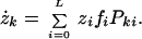1

The value f_i denotes the fitness of a genome with i mutations, and P_ki is the probability of mutation from an i-error genotype to a k-error genotype during replication (see Appendix). L denotes genome length.

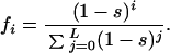
We consider multiplicative fitness landscapes of the form f_i ∝ (1 − s)ⁱ. The wild-type sequence, i = 0, is maximally fit, and each deleterious mutation reduces fitness by an amount (1 − s), independent of the other loci. The parameter s measures the deleteriousness of each mutation; this selective value is usually very small. By varying the magnitude of s we vary the steepness of the landscape and hence the effective degree of redundancy in the genome (Fig. 1).

Figure 1.

A schematic diagram of fitness landscapes with different degrees of redundancy. The x–y plane denotes the space of genotypes and the x axis denotes the corresponding fitness. High values of landscape steepness, s, correspond to antiredundant genomes (Lower Right) for which single mutations lead to considerable reductions in fitness. Smaller values of s correspond to shallower landscapes (Upper Left) and increasing degrees of redundancy. All landscapes are normalized to have the same total volume (Eq. 2); shallower landscapes have shorter wild-type peaks.

To compare different mean fitness values for different levels of redundancy (s), we normalize so that the sum of all fitness classes is unity:

2

This normalization ensures that genotypes cannot evolve toward both maximum fitness and maximum redundancy simultaneously. The normalization enforces a tradeoff between the absolute height of the landscape and its steepness. The existence of such a tradeoff follows from molecular considerations. Molecular mechanisms of redundancy impose fitness costs on the wild type, through increased genome size, increased metabolism, or reduced binding specificity. Although the precise form of the tradeoff curve is arbitrary and relatively unimportant (other normalizations yield similar results), it is essential that we impose some tradeoff between maximum fitness and redundancy.

Unlike most treatments of the quasispecies equation, we must here allow for back mutations. According to two famous principles of population genetics, the neglect of back mutations introduces pathologies into the equilibrium state of both infinite and finite populations. If back mutations are neglected then, according the Haldane–Muller principle, the mean equilibrium fitness of an infinite haploid population is independent of the landscape's steepness (19). If back mutations are ignored in small populations, on the other hand, Muller's ratchet implies that mean fitness will tend always toward a minimum, regardless of the landscape steepness. (The landscape steepness can affect the speed, but not the eventual outcome, of Muller's ratchet.) To detect adaptive benefits or costs of redundancy, therefore, we cannot ignore back mutations.

We are assuming a form of redundancy produced by a genetic network property with, on average, an equal contribution from each gene (20, 21). We do not model the explicit mechanism of redundancy (see Table 1) but rather explore the generic consequences of redundancy on mean fitness. In the Appendix, we derive the average number of mutations, k̄, for a genotype in mutation-selection equilibrium. This yields the following approximation for mean population fitness:

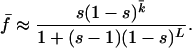3

For small population sizes, the deterministic quasispecies equation does not apply. In this case, however, moment equations (22) can be used to express the mean fitness as a function of the effective population size N (see Appendix). These equations determine the relationship between mean population fitness, the strength of selection, the rate of mutation, the genome length, and the size of the population. Recent studies (18) have emphasized the role of mutation in selecting for flatter landscapes; we emphasize the role of population size.

Table 1.

A summary of mechanisms responsible for creating redundancy and antiredundancy at the cellular level

Redundancy	Antiredundancy
Gene duplication (14)	Overlapping reading frames (9)
Neutral codon usage (25)	Nonconservative codon bias (26)
—	Gene silencing (27)
Polyploidy (28)	Haploidy
Multiple regulatory elements for n genes (29)	Single regulatory element for n genes
Chaperone and heat shock proteins (30, 31)	—
Checkpoint genes promoting repair (32)	Checkpoint genes inducing apoptosis (33)
Telomerase induction (34)	Loss of telomerase (35)
Dominance (36, 37)	Incomplete dominance
Autophagy (38, 39)	—
mRNA surveillance (40, 41)	—
Bulk transmission (42, 43)	Bottlenecks in transmission (44, 45)
Molecular quality control (46)	—
tRNA suppressor molecules (47)	—
Modularity (48)	—
Multiple organelle copies (49)	Single organelle copies
Parallel metabolic pathways (6, 50)	Serial metabolic pathways
Correlated gene expression (29, 51)	Uncorrelated gene expression
DNA error repair (52)	Loss of error repair (53–55)

Redundant mechanisms mask the phenotypic effect of mutations, allowing the mutations to persist in populations. We group together these mechanisms with a small s value. Antiredundant mechanisms increase the efficiency of local selection to remove damaged components, and are associated with large s values. These diverse biological processes illustrate a range of mechanisms through which evolution can modify the redundancy of genotypes. Reference numbers are given in parentheses. 

The Influence of Population Size

Fig. 2 shows the relationship between level of redundancy and expected mean fitness for several different population sizes. Both in theory (Fig. 2a) and in individual-based stochastic simulations (Fig. 2b) we see that redundancy increases the mean fitness in small populations, whereas it decreases fitness in large populations. This central result has an intuitive explanation. In small populations, mutational drift contributes disproportionately to the population fitness. There is a large temporal variance in the mean hamming class, and redundancy can effectively mask these mutations. Small populations are thus better served by shallow landscapes—i.e., by slightly decreasing the fitness of the wild type, but increasing the fitness of its nearby neighbors. Large populations, however, are not at risk of being “swept off” the fitness peak by the stochastic fluctuations that afflict small populations; the temporal variance in the mean hamming class is small. It is better, therefore, for large populations to amplify the phenotypic penetrance of deleterious genes by means of sharp landscapes.

Figure 2.

(a) The theoretical relationship between redundancy and equilibrium mean fitness for populations of various sizes (N = 10, 100, 500, 1,000, 10,000, and N infinite). Small populations benefit from redundant (i.e., flatter) landscapes, but large populations prefer antiredundant (i.e., steeper) landscapes. The curves in the figure, given by Eqs. 3, 6, and 7, correspond to genome length L = 10⁴ and mutation rate u = 5 ⋅ 10⁻⁵. (b) The relationship between redundancy and equilibrium mean fitness as observed from individual-based computer simulations of the quasispecies equation (L = 1,000, u = 5 ⋅ 10⁻⁴). Each individual is characterized by its hamming distance from wild type. The mean population fitness is computed by averaging the last 20% of 10,000 generations with selection and mutation. In each discrete generation, N parents are chosen probabilistically from the previous generation according to their relative fitnesses. The offspring of a parent is mutated according to Eq. 5. The numerical studies confirm the theoretical prediction: small populations prefer shallow landscapes, whereas large populations prefer steep landscapes.

Our results on equilibrium mean population fitness (Fig. 2) constitute a population-based argument for the evolution of redundancy in small populations and antiredundancy in large populations. These results do not, in themselves, demonstrate that such strategies are evolutionarily stable or achievable. In other words, we must yet demonstrate that individual replicators subject to individual-level selection evolve degrees of redundancy consistent with the optimal population mean fitness. If we allow individuals to modify the heritable steepness of their own individual landscapes through mutation, however, we find that small populations do, indeed, evolve toward redundancy, and large populations evolve toward antiredundancy by means of individual-level selection (Fig. 3). For both population sizes, the evolution toward the preferred level of redundancy is punctuated or episodic.

Figure 3.

The evolution of redundancy in a small population (Upper) and of antiredundancy in a large population (Lower). We perform quasispecies simulations in which individuals are characterized both by their hamming class k and their individual landscape steepness s. We choose genome size L = 500 and per-base mutation rate u = 0.001. On a slow time scale (probability 0.0005 per replication), an individual's landscape is heritably mutated (uniformly within [s − 0.005, s + 0.005]). For the small population, all individuals begin as wild types with a fairly steep landscape, s = 0.05. For the large population, all individuals begin as wild types with s = 0.025. After an initial transient, in both cases the population's mean landscape steepness s̄ evolves toward its preferred level. Simultaneously, the mean population fitness f̄ increases; although it increases less dramatically for the small population. Throughout the evolutionary time course, the within-population variance in redundancy (σ²) is small. In addition, over time the small population becomes delocalized (k̄ increases), whereas the large population becomes increasingly localized (data not shown).

The evolutionary stability of these two strategies—sensitivity in large populations and redundancy in small populations—has an intuitive explanation. The stability rests on the fact that flatter landscapes have lower fitness peaks. A large population on a steep landscape is highly localized near the wild type (low k̄). Mutants with different s-values are thus most often generated near the wild type—precisely where a more shallow landscape would be disadvantageous to them. Conversely, small populations with shallow landscapes are delocalized (high k̄). In this case, landscape mutants tend to arise far from the wild type—precisely where a steeper landscape would decrease their fitness. Thus, the landscape itself acts as a mechanism for ensuring the robustness of the incumbent strategy, in each population size.

Redundant and Antiredundant Mechanisms in Biology

We have shown how population size influences the degree of redundancy expressed by a genome. In large populations of viruses and bacteria, and in large populations of rapidly dividing cells within multicellular organisms, we expect an evolution toward antiredundant mechanisms. For small populations, on the other hand, we expect a tendency toward redundancy. Table 1 lists a variety of molecular mechanisms capable of producing redundancy and antiredundancy. Our quasispecies model provides a statistical treatment of the parameter s that is the developmental end-point of each of these particular mechanisms. The mechanisms in Table 1 all influence development and somatic processes by modifying the effective degree of deleteriousness, s, of mutations.

Antiredundant mechanisms (high s values) include overlapping reading frames, absence of tRNA suppressor genes, codon bias, loss of DNA error repair, reduced number of promoters, coordinated expression of genes, and checkpoint genes. All of these mechanisms remove mutant genomes from populations (either of individuals or cells). Redundant mechanisms (low s values) include duplicated genes, correlated gene functions, tRNA suppressors, heat shock proteins, molecular quality control, and alternative metabolic pathways. These mechanisms, which incur a cost (through increased genome size or greater need for resources), mask the effects of mutation. When available, both redundant and antiredundant strategies can be exploited, even simultaneously, by a single organism. Strategies may also vary according to cell types.

Redundancy and Levels of Selection

The dynamics of redundancy and antiredundancy reveal an intriguing interplay between the “levels of selection.” In multicellular organisms, rapidly dividing cells experience selection, in effect, as members of a large quasispecies—much like viruses or bacteria. Large multicellular organisms often experience relatively small population sizes, though the cells of which they are composed experience huge population sizes. Hence there is a possible conflict between the organismal and cellular levels of selection: the multicellular organism would benefit from a redundant (flatter) fitness landscape, whereas the cells of which the organism is composed would benefit from an antiredundant (steeper) landscape. Interestingly, in some cases this conflict has a synergistic resolution: antiredundancy at the cellular level is an effective means of ensuring redundancy and robustness at the organismal level. Antiredundant mechanisms activated in mutant or damaged cells cause their removal, thereby ensuring stability (redundancy) against mutation in tissues.

Both the large cellular population within an individual and the smaller population of individuals themselves can increase their mean fitness by adopting these apparently conflicting strategies. There are four combinations of strategies available: (i) redundancy at the cellular level promoting redundancy at the organismal level (for example, polyploidy); (ii) redundancy at the cellular level promoting antiredundancy at the organismal level (loss of molecular checkpoints); (iii) antiredundancy at the cellular level promoting redundancy at the organismal level (checkpoint genes inducing apoptosis); and (iv) antiredundancy at the cellular level promoting antiredundancy at the organismal level (bottlenecks in organelle transmission within and between generations). The favored strategy depends on the local population size experienced by cell and organism. Because our model does not separate germ line from soma, we cannot directly address a true evolutionary conflict of interest between cells and organism. Mammalian cancer provides such an example. Mutated cells strive to increase cellular redundancy to avoid the cost of their mutations, thereby damaging the organism. The organism seeks to promote cellular antiredundancy so as to remove mutant cells and increase organismal redundancy (case iii). Antiredundancy at the cellular level should be viewed as a victory for organismal selection.

Analogous to the cells of a complex organism, viruses, bacteria, and mitochondria often exhibit antiredundant mechanisms as a consequence of their large populations and selection for compressed genomes. Once again, antiredundant mechanisms at the individual level can increase the mean fitness and stabilize the quasispecies as a whole.

Redundancy and Cell Type

Finally, our theory predicts that, within a complex differentiated organism, the level or redundancy expressed within each cell type will depend on the effective reproducing population size the cell type in question. For example, human brain cells seldom regenerate and thus have an extremely small effective population size. As a result, antiredundant mechanisms, such as apoptosis, are strongly inhibited, whereas redundant mechanisms, including the chaperones, are highly expressed (23). The same logic implies that the amount of redundancy found within gene families will depend on the effective population size of the selective unit at which those genes operate. Housekeeping genes code for processes important at the single cell level. Because individual cells are present in large population sizes, functionally redundant copies of housekeeping genes should be rare. Conversely, genes involved in immune-system regulation encode functions operating at the organismal level, where population sizes are often much lower. We would expect that these genes have many backup copies (7). The predicted level of redundancy requires that we identify the effective population size at which genes come under strongest selection.

Appendix

Eigen's quasispecies framework considers a large population of L-bit genomes, x_i, reproducing with imperfect fidelity according to their fitnesses, w_i, with fixed total concentration:

4

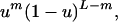
In this equation, W(t) = ∑w_jx_j(t) denotes the mean population fitness. The mutation matrix Q_ij is determined by the per-base mutation rate, u, and the hamming distance H(i,j) between genome i and j: Q_ij = u^H(i,j)(1 − u)^L−H(i,j).

When the fitness depends only on hamming class, the number of equations is dramatically reduced (Eq. 1) by considering the evolution of all k-error mutants together: z_k = ∑_H(i) = _kx_i. The chance of mutation from class l to class k is given by

5

where we include only terms for which k + m ≡ l (mod 2). In this formulation, the forward and backward mutation rates are equal. All of our qualitative results (Figs. 2b and 3) remain unchanged, however, even if forward mutations occur at twice the rate of backward mutations.

We consider multiplicative fitness landscapes of the form f_k ∝ (1 − s)^k (Eq. 2). For s small, this multiplicative formulation is the prototypical example of a nonepistatic landscape (16, 17), which has the advantage of analytic tractability. All of our qualitative results (Figs. 2b and 3) remain essentially unchanged, however, if landscapes contain moderate synergistic or antagonistic epistasis: f_k ∝ (1 − s)^kα, for 0.8 < α < 1.2.

The dominant eigenvector of (f_lP_kl) provides the equilibrium relative abundances of the hamming classes. Moreover, the corresponding dominant eigenvalue equals the equilibrium mean fitness. As suggested in ref. 24, we look for an eigenvector of the binomial form z_k = ()a^k (1 − a)^L−k, where a must yet be determined. To compute a, we solve the discrete-time equivalent of Eq. 4, which reduces to the same eigensystem problem (24). Given the current abundances of hamming classes (z₀, z₁, … , z_L), consider the random variable V defined by the hamming class after mutation of an individual chosen from the population according to its relative fitness. The generating function of V,

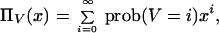where x is a formal variable, is given by Π_V(x) = ∑_k z_kf_k ⋅ [u + (1 − u)x]^k ⋅ [(1 − u) + ux]^L−k. In equilibrium we have Π_V(x) = λ ∑ z_kx^k, which, on the binomial substitution, determines the value of a:

6

In equilibrium, the mean hamming distance from the wild type is k̄ = aL.

According the moment equations of Woodcock and Higgs (24), when u is small the following expression approximates the equilibrium mean hamming class in a population of size N:

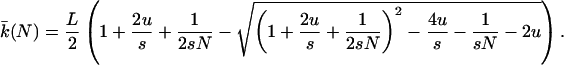7

Substitution into Eq. 3 yields the equilibrium mean fitness.

References

- 1.Tautz D. BioEssays. 1992;14:263–266. doi: 10.1002/bies.950140410. [DOI] [PubMed] [Google Scholar]
- 2.Gibson G, Wagner G. BioEssays. 2000;22:372–380. doi: 10.1002/(SICI)1521-1878(200004)22:4<372::AID-BIES7>3.0.CO;2-J. [DOI] [PubMed] [Google Scholar]
- 3.Maconochie M, Nonchev S, Morrison A, Krumlauf R. Annu Rev Genet. 1996;30:529–556. doi: 10.1146/annurev.genet.30.1.529. [DOI] [PubMed] [Google Scholar]
- 4.Li X, Noll M. Nature (London) 1994;367:83–87. doi: 10.1038/367083a0. [DOI] [PubMed] [Google Scholar]
- 5.Hoffmann F M. Trends Genet. 1991;7:351–355. doi: 10.1016/0168-9525(91)90254-f. [DOI] [PubMed] [Google Scholar]
- 6.Normanly J, Bartel B. Curr Opin Plant Biol. 1999;2:207–213. doi: 10.1016/s1369-5266(99)80037-5. [DOI] [PubMed] [Google Scholar]
- 7.Williamson A R, Premkumar E, Shoyab M. Fed Proc. 1975;34:28–32. [PubMed] [Google Scholar]
- 8.Krakauer D C, Nowak M A. Semin Cell Dev Biol. 1999;10:555–559. doi: 10.1006/scdb.1999.0337. [DOI] [PubMed] [Google Scholar]
- 9.Krakauer D C. Evolution (Lawrence, Kans) 2000;54:731–739. doi: 10.1111/j.0014-3820.2000.tb00075.x. [DOI] [PubMed] [Google Scholar]
- 10.Levine A J. Cell. 1997;88:323–331. doi: 10.1016/s0092-8674(00)81871-1. [DOI] [PubMed] [Google Scholar]
- 11.Aragona M, Maisano R, Panetta S, Giudice A, Morelli M, La Torre I, La Torre F. Int J Oncol. 2000;17:981–989. doi: 10.3892/ijo.17.5.981. [DOI] [PubMed] [Google Scholar]
- 12.Lynch M, Burger R, Butcher D, Gabriel W. J Hered. 1993;84:339–344. doi: 10.1093/oxfordjournals.jhered.a111354. [DOI] [PubMed] [Google Scholar]
- 13.Wagner A. J Evol Biol. 1999;12:1–16. [Google Scholar]
- 14.Nowak M A, Boerlijst M C, Cooke J, Smith J M. Nature (London) 1997;388:167–171. doi: 10.1038/40618. [DOI] [PubMed] [Google Scholar]
- 15.Eigen M. Naturwissenschaften. 1971;58:465–523. doi: 10.1007/BF00623322. [DOI] [PubMed] [Google Scholar]
- 16.Burger R. The Mathematical Theory of Selection, Recombination, and Mutation. New York: Wiley; 2000. [Google Scholar]
- 17.Chao L. J Theor Biol. 1988;133:99–112. doi: 10.1016/s0022-5193(88)80027-4. [DOI] [PubMed] [Google Scholar]
- 18.Wilke C, Wang J, Ofria C, Lenski R, Adami C. Nature (London) 2001;412:331–333. doi: 10.1038/35085569. [DOI] [PubMed] [Google Scholar]
- 19.Kimura M, Maruyama T. Genetics. 1996;57:21–34. [Google Scholar]
- 20.Bornholdt S, Sneppen K. Proc R Soc London B. 2000;267:2281–2286. doi: 10.1098/rspb.2000.1280. [DOI] [PMC free article] [PubMed] [Google Scholar]
- 21.Wagner A. Nat Genet. 2000;24:355–361. doi: 10.1038/74174. [DOI] [PubMed] [Google Scholar]
- 22.Higgs P G. Genet Res Camb. 1994;63:63–78. [Google Scholar]
- 23.Cummings C J, Sun Y, Opal P, Antalffy B, Mestril R, Orr H T, Dillmann W H, Zoghbi H Y. Hum Mol Genet. 2001;10:1511–1518. doi: 10.1093/hmg/10.14.1511. [DOI] [PubMed] [Google Scholar]
- 24.Woodcock G, Higgs P G. J Theor Biol. 1996;179:61–73. doi: 10.1006/jtbi.1996.0049. [DOI] [PubMed] [Google Scholar]
- 25.Freeland S J, Hurst L D. J Mol Evol. 1998;47:238–248. doi: 10.1007/pl00006381. [DOI] [PubMed] [Google Scholar]
- 26.Berg O G, Silva P J. Nucleic Acids Res. 1997;25:1397–1404. doi: 10.1093/nar/25.7.1397. [DOI] [PMC free article] [PubMed] [Google Scholar]
- 27.Gottschling D E. Curr Biol. 2000;10:R708–R711. doi: 10.1016/s0960-9822(00)00714-4. [DOI] [PubMed] [Google Scholar]
- 28.Otto S P, Whitton J. Annu Rev Genet. 2000;34:401–437. doi: 10.1146/annurev.genet.34.1.401. [DOI] [PubMed] [Google Scholar]
- 29.Siefert J L, Martin K A, Abdi F, Widger W R, Fox G E. J Mol Evol. 1997;45:467–472. doi: 10.1007/pl00006251. [DOI] [PubMed] [Google Scholar]
- 30.Ohtsuka K, Hata M. Int J Hyperthermia. 2000;16:231–245. doi: 10.1080/026567300285259. [DOI] [PubMed] [Google Scholar]
- 31.Macario A J, Lange M, Ahring B K, De Macario E C. Microbiol Mol Biol Rev. 1999;63:923–967. doi: 10.1128/mmbr.63.4.923-967.1999. [DOI] [PMC free article] [PubMed] [Google Scholar]
- 32.Weinert T A, Kiser G L, Hartwell L H. Genes Dev. 1994;8:652–665. doi: 10.1101/gad.8.6.652. [DOI] [PubMed] [Google Scholar]
- 33.Hartwell L. Cell. 1992;71:543–546. doi: 10.1016/0092-8674(92)90586-2. [DOI] [PubMed] [Google Scholar]
- 34.Meyerson M. J Clin Oncol. 2000;18:2626–2634. doi: 10.1200/JCO.2000.18.13.2626. [DOI] [PubMed] [Google Scholar]
- 35.Urquidi V, Tarin D, Goodison S. Annu Rev Med. 2000;51:65–79. doi: 10.1146/annurev.med.51.1.65. [DOI] [PubMed] [Google Scholar]
- 36.Bourguet D. Heredity. 1999;83:1–4. doi: 10.1038/sj.hdy.6885600. [DOI] [PubMed] [Google Scholar]
- 37.Hurst L D, Randerson J P. J Theor Biol. 2000;205:641–647. doi: 10.1006/jtbi.2000.2095. [DOI] [PubMed] [Google Scholar]
- 38.Hunziker W, Geuze H J. BioEssays. 1996;18:379–389. doi: 10.1002/bies.950180508. [DOI] [PubMed] [Google Scholar]
- 39.Liang X H, Jackson S, Seaman M, Brown K, Kempkes B, Hibshoosh H, Levine B. Nature (London) 1999;402:672–676. doi: 10.1038/45257. [DOI] [PubMed] [Google Scholar]
- 40.Cali B M, Anderson P. Mol Gen Genet. 1998;260:176–184. doi: 10.1007/s004380050883. [DOI] [PubMed] [Google Scholar]
- 41.Cali B M, Kuchma S L, Latham J, Anderson P. Genetics. 1999;151:605–616. doi: 10.1093/genetics/151.2.605. [DOI] [PMC free article] [PubMed] [Google Scholar]
- 42.Novella I S, Elena S F, Moya A, Domingo E, Holland J J. J Virol. 1995;69:2869–2872. doi: 10.1128/jvi.69.5.2869-2872.1995. [DOI] [PMC free article] [PubMed] [Google Scholar]
- 43.Chao L. J Theor Biol. 1991;153:229–246. doi: 10.1016/s0022-5193(05)80424-2. [DOI] [PubMed] [Google Scholar]
- 44.Bergstrom C T, Pritchard J. Genetics. 1998;149:2135–2146. doi: 10.1093/genetics/149.4.2135. [DOI] [PMC free article] [PubMed] [Google Scholar]
- 45.Jansen R P, de Boer K. Mol Cell Endocrinol. 1998;145:81–88. doi: 10.1016/s0303-7207(98)00173-7. [DOI] [PubMed] [Google Scholar]
- 46.Vallee F, Lipari F, Yip P, Sleno B, Herscovics A, Howell P L. EMBO J. 2000;19:581–588. doi: 10.1093/emboj/19.4.581. [DOI] [PMC free article] [PubMed] [Google Scholar]
- 47.Buvoli M, Buvoli A, Leinwand L A. Mol Cell Biol. 2000;20:3116–3124. doi: 10.1128/mcb.20.9.3116-3124.2000. [DOI] [PMC free article] [PubMed] [Google Scholar]
- 48.Ancel L W, Fontana W. J Exp Zool. 2000;288:242–283. doi: 10.1002/1097-010x(20001015)288:3<242::aid-jez5>3.0.co;2-o. [DOI] [PubMed] [Google Scholar]
- 49.Chomyn A, Martinuzzi A, Yoneda M, Daga A, Hurko O, Johns D, Lai S T, Nonaka I, Angelini C, Attardi G. Proc Natl Acad Sci USA. 1992;89:4221–4225. doi: 10.1073/pnas.89.10.4221. [DOI] [PMC free article] [PubMed] [Google Scholar]
- 50.Bruggeman F J, van Heeswijk W C, Boogerd F C, Westerhoff H V. Biol Chem. 2000;381:965–972. doi: 10.1515/BC.2000.119. [DOI] [PubMed] [Google Scholar]
- 51.Normark S, Bergstrom S, Edlund T, Grundstrom T, Jaurin B, Lindberg F P, Olsson O. Annu Rev Genet. 1983;17:499–525. doi: 10.1146/annurev.ge.17.120183.002435. [DOI] [PubMed] [Google Scholar]
- 52.Strauss B S. Life Sci. 1974;15:1685–1693. doi: 10.1016/0024-3205(74)90171-4. [DOI] [PubMed] [Google Scholar]
- 53.Strauss B S. Semin Cancer Biol. 1998;8:431–438. doi: 10.1006/scbi.1998.0092. [DOI] [PubMed] [Google Scholar]
- 54.Strauss B S. Perspect Biol Med. 2000;43:286–300. doi: 10.1353/pbm.2000.0010. [DOI] [PubMed] [Google Scholar]
- 55.Domingo E. Virology. 2000;270:251–253. doi: 10.1006/viro.2000.0320. [DOI] [PubMed] [Google Scholar]