The Combined Focal Cross Entropy and Dice Loss Function for Segmentation of Protein Secondary Structures from Cryo-EM 3D Density maps

Abstract

Although cryo-electron microscopy (cryo-EM) has been successfully used to derive atomic structures for many proteins, it is still challenging to derive atomic structure when the resolution of cryo-EM density maps is in the medium resolution range such as 5–10 Å. Although multiple neural networks have been proposed for the problem of secondary structure detection from cryo-EM 3D images, loss functions used in the existing networks are primarily based on cross entropy loss (CE). In order to study the behavior of various loss functions in the secondary structure detection problem, we investigated five loss functions and compared their performances. Using a U-net architecture in DeepSSETracer and a test set of 65 protein chains of atomic structures and their corresponding cryo-EM density component maps, we found that the combined function with focal cross entropy loss (FCE) and Dice loss (DL) provides the best overall detection of secondary structures. In particular, the combined loss function has a significant enhancement of an overall F₁ score of 6.7% when compared to CE in detection of β-sheet voxels that are generally much harder to be detected accurately than for helix voxels. Our work shows the potential of designing effective loss functions to enhance the detection of hard cases in the segmentation of secondary structure problem.

I. Introduction

A cryo-electron microscopy (cryo-EM) density map is a 3-dimensional image, in which the value at each voxel represents the local density of electrons. The challenges to derive protein atomic structures from cryo-EM density maps depend on the resolutions of the maps. With the advance of cryo-EM technology, many cryo-EM density maps with 2 to 4Å resolutions have been produced in the last ten years. At such resolutions, details about the backbone and some amino acid side chains are often resolved, and atomic structures can be derived. Cryo-EM has become a routine technology to derive atomic resolutions for many molecular complexes [1, 2]. However, for cryo-EM density maps with a medium resolution (5–10 Å), not only side chain details are mostly not distinguishable, it is often challenging to recognize the backbone of the protein chain. In most cases, it is not possible to derive atomic structures from these medium resolution images without the knowledge of known atomic structures as templates. When a template structure is available from the Protein Data Bank (PDB), the atomic structure is often derived through fitting [3, 4]. When no suitable template structures are available, possible configurations of the backbone may be suggested through matching secondary structures that are detected from the 3D image and those predicted from the amino acid sequence [5–7]. Medium-resolution cryo-EM density maps have been steadily deposited in Electron Microscopy Data Bank (EMDB). With current advances of cryo-electron tomography and subtomogram averaging techniques, more density maps about cellular organelles are expected to reach medium resolution.

In order to derive atomic structures from medium-resolution density maps, it is important to know the location of secondary structures in such maps. Secondary structures, such as α-helices and β-sheets, are major building blocks of a protein, and their relative location in the 3D volume of a density map provides constraints in deriving the backbone of a protein structure. An example of the atomic structure of a protein chain (ribbon), with helices (yellow ribbon) and β-sheets (cyan ribbon), and its corresponding component density map (gray) at medium resolution is shown in Figure 1A. The problem of secondary structure segmentation is to detect helix region and β-sheet regions from the density map. An example of segmented helix (yellow) and β-sheet regions (cyan) from a medium-resolution map is shown in Figure 1D.

Fig.1.

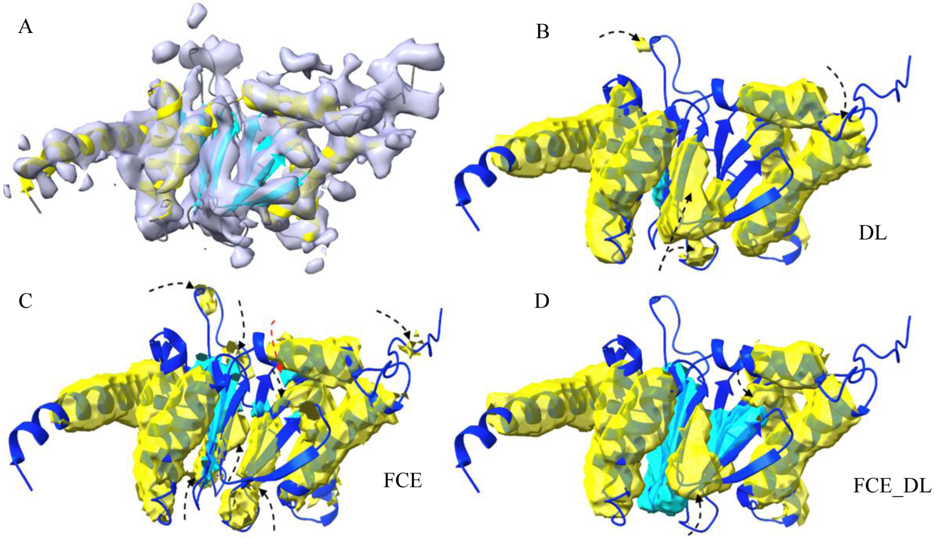
Segmentation of secondary structures using CNN with FCE, DL and FCE_DL loss functions. (A): The cryo-EM density map (EMD-4089, grey) component corresponding to the atomic structure of chain D of 5ln3 (PDB ID, ribbon); Helices (yellow ribbon) and β-sheets (cyan ribbon) are indicated for the atomic structure. Helix regions (yellow) and β-sheet regions (cyan) that were detected using DL (B), FCE (C), and combined loss function FCE_DL (D) are superimposed with the atomic structure (blue ribbon). Some wrongly detected regions of helix and β-sheet are indicated using black and red arrows respectively. (C) Note that β-sheet is better predicted using FCE_DL in (D).

Although multiple image processing and machine learning methods have been developed detecting secondary structures from medium-resolution cryo-EM density maps [8–14], recent deep learning approaches show good potential [15–18]. One of the persisting challenges in existing methods is accurate detection of β-sheet regions. Several characters of β-sheets potentially contribute to the challenge, such as their lower density range, in general, than that of helices, varying shapes and sizes. In some cases, it is hard to distinguish a β-sheet, since the dense subregion of a β-sheet may appear cylindrical and hence is mistakenly recognized as a helix (arrow in Figure 2A). In addition, small β-sheets, such as those containing only two short β-strands (arrow, Figure 3A) are generally hard to be detected. A recent study shows that an average residue-level F₁ score of 72% was obtained for detection of helices using DeepSSETracer, but only F₁ score of 65% was obtained for detection of β-sheets [18]. A lower F₁ score for β-sheet detection was also observed, 77% for helix and 42% for β-sheet detection, when a different method, Emap2sec+ [16], was used [18].

Fig.2.

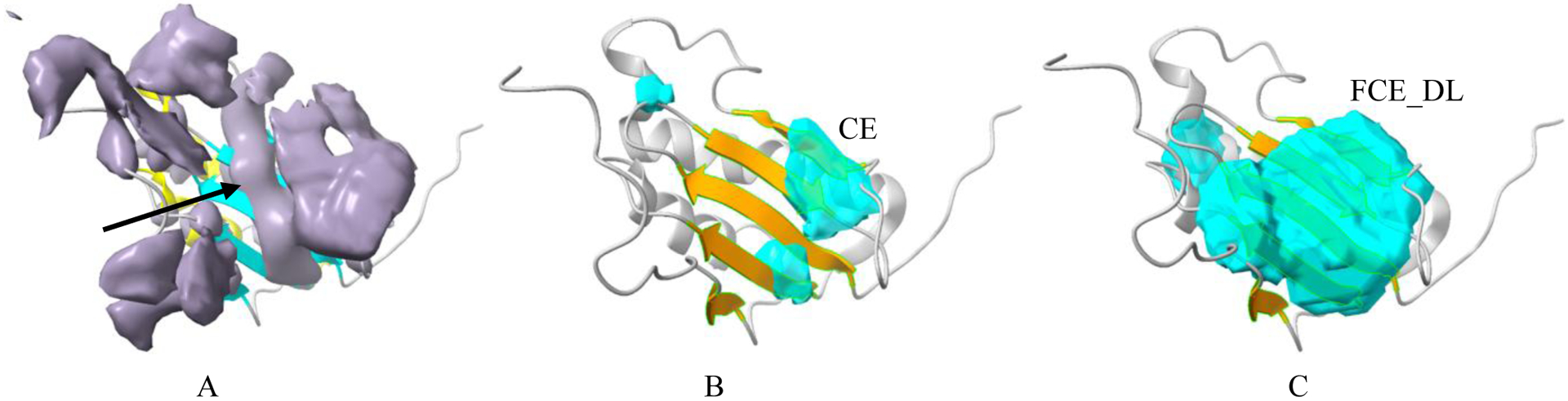
Detection of β-sheet region for a hard case using CE and FCE_DL loss functions. (A): The cryo-EM density map (EMD-3581, grey) component corresponding to the atomic structure of chain AK of 5myj (PDB ID, cyan ribbon for β-sheet and yellow ribbon for helix). A subregion of β-sheet (arrow) appears as a cylindrical helix. β-sheet regions (cyan) that were detected using cross entropy loss function CE (B) and combined loss function FCE_DL (C) are superimposed with the atomic structure where β-sheet is colored orange.

Fig.3.

Segmentation of a small β-sheet using CE, FCE, DL, and FCE_DL loss functions. The segmented β-sheet regions (cyan) from the cryo-EM density map (EMD-6456) component corresponding to the atomic structure of chain AL of 3jbn (PDB ID, ribbon). A small β-sheet (arrow) contains two short β-strands (orange ribbon). β-sheet regions (cyan) that were detected using CE (A), FCE (B), DL (C), and the combined loss function FCE_DL (D) are superimposed with the atomic structure (β-strands colored in gold).

Although multiple deep learning methods have been proposed for the secondary structure detection problem, there is limited study to understand the effectiveness of important network elements. A loss function is an important element in the deep learning framework. Depending on the application domain, it is possible that certain designs of loss functions provide better learning outcomes than others. Cross entropy (CE) is a popular loss function used in many learning problems. It is also used in secondary structure segmentation methods, such as EMap2sec+ and EMNUSS [16, 17]. However, it is known for its weakness handling class imbalance [19]. More specially, the model trained with cross entropy tends to perform poorly on voxels from the class with fewer voxels, even though the overall accuracy is relatively good. Dice loss (DL) is another popular function used in medical image problems [20]. Compared to cross entropy, Dice coefficient is less sensitive to class imbalance (especially the imbalance between foreground and background voxels), but it is less smooth, thus difficult to optimize. In previous works, both cross entropy and Dice coefficient have been individually used as the optimization objective in image segmentation when a U-Net like fully convolutional neural network (CNN) was used [21–23]. Focal cross entropy loss have been recently proposed in Lin et al. [19]. It is designed to down-weight the loss from easy examples. Focal Dice loss was also proposed in Prencipe et al. to incorporate the idea of focal cross entropy loss with the Dice loss [24].

In cryo-EM density maps, or 3D images, different kinds of regions can often be visually recognized with varying difficulty. Depending on how data are pre-processed from an entire cryo-EM map, training data may contain large areas not related to molecules. Those voxels not related to molecular mass are generally easiest to be distinguished, followed by helix regions, since they have the most obvious characters than for β-sheets and loops. The shape of a β-sheet varies depending on the kind of β-sheet and local environment, and therefore β-sheets are much harder to be detected accurately by any currently available methods than for helices. In addition, the content of helices/β-sheets in an image varies from image to image. Some protein chains have only helices and no β-sheets, some have only β-sheets. The varying level of difficulty and the abundance of patterns in the training data provide interesting problems to design a loss function that considers the strength of the patterns. Class imbalance is a common problem in deep learning. In this study, we utilized our previous U-net like architecture in DeepSSETracer [18], but the work particularly focuses on the effect of different loss functions to segment secondary structures from cryo-EM density maps. This is the first study attempt to understand the effectiveness of an important neural network element in segmentation of secondary structure from cyro-EM images. Results may provide insights to future design of the network and training framework. Our results from 65 test cases show that although focal cross entropy loss and Dice loss functions show enhanced performance than cross entropy function, the combined focal cross entropy and Dice loss function shows the best performance. The major enhancement is in detection of β-sheets, the most difficult class among the three. An overall F₁ score improved 6.7% when the combined focal cross entropy and Dice loss function was used, in comparison with the use of the cross entropy loss.

II. Methods

A. Dataset and Architecture

The dataset involves 1268 protein chains for training, 49 chains for validation and 65 chains for testing. Each protein chain in the data set contains a pair of atomic structure and its corresponding 3D image. Cryo-EM density maps of resolution between 5 and 10 Å were downloaded from EMDB, and their corresponding atomic structures were downloaded from PDB. The dataset was selected using averaged helix cylindrical similarity score of a chain to eliminate low-quality pairs, in which the image and the structure are not well aligned [25]. A density map is often associated with multiple chains of one or more proteins, but individual chains and their corresponding density area were used in training and testing. The atomic structure of individual chains of proteins were used as envelopes to extract the chain-containing density regions using Chimera [26] and a parameter of 5Å radius around each atom. Since it is common to see multiple copies of the same sequence in a cryo-EM density map, duplicated copies in each protein were removed from the pool to reduce training bias. Needleman-Wunsch algorithm was used to align a pair of sequences, and near identical chains (i.e., with more than 70% sequence identity) in the same protein were removed. The details about the generation of labels and the adopted neural network architecture can be found in Mu et al. [18]. For a summary, the architecture contains five composite layers. It was adapted from the 3D U-Net [22], and it takes input of 4D tensors of different sizes.

Three classes were used to represent helix, β-sheet, and background voxels, respectively. The background voxels are non-helix, non-sheet voxels, containing both non-molecular voxels and those in loops and turn regions of molecules. The voxels not related to molecules were mostly created in the data extraction step where a molecular mask was used to extract the region only corresponding to the chain. The resulting distribution of classes show severe imbalance with only about 2.4% of voxels in helix regions, and about 1% voxels in β-sheet regions. About 96.6% of the overall voxels are background voxels. In this paper, we discuss the effect of various loss functions to deal with such data with severe imbalance and different levels of difficulty in patterns.

B. Loss Functions

In order to search for an effective loss function for the dataset with severe class imbalance, we explored three single-term loss functions: cross entropy, focal cross entropy, and dice, and two composite loss functions: one is the combination of cross entropy and dice and the other one is that of focal cross entropy and dice.

For each image in our study, as it is in 3D, both the true label and the prediction are 4D volumes with the fourth dimension representing the K different class labels and the rest representing height, width and depth (z-direction), respectively. Let $y^{<i,j>}$ be the binary vector of length $K$ that represents the true label of the $j\_th$ voxel in the $i\_th$ image. Since the class assignment of labels for any voxel is mutually exclusive, only one of the K entries in $y^{<i,j>}$ is 1 and all the rest are 0’s. Let $p^{<i,j>}$ be the vector of ($p_1^{<i,j>}, \cdots , p_k^{<i,j>}$) where $p_k^{<i,j>}$ denotes predicted probability of $\mathit{\text{voxel}}<i, j>$ belonging to class $k=1,\cdots , K$. With these notations, each of the five explored loss functions is defined in below.

Cross Entropy (CE) Loss

$$\mathit{\text{CE}}\left(𝒴,𝒫\right)=-{\sum }_{i=1}^N{\sum }_{j=1}^{N^i}{\sum }_{k=1}^K{y}_k^{<i,j>}\mathit{\text{log}}{p}_k^{<i,j>}.$$

where$𝒴=\left\{y^{<i,j>}\right\}, 𝒫=\left\{p^{<i,j>}\right\} \mathit{\text{with}} i\in \left\{1,\cdots , N\right\}, j\in \left\{1,\cdots , N^i\right\}$. N is the total number of images in the training set, $N^i$ is the total number of voxels in $i\_\mathit{\text{th}}$ image, $y_k^{<i,j>}$ and $p_k^{<i,j>}$ represent the $k\_\mathit{\text{th}}$ entry $y^{<i,j>}$ and $p^{<i,j>}$ respectively. For each voxel, $p^{<i,j>}$ is computed by passing the activation ($a^{<i,j>}$) of the last convolution block (i.e., conv|BN|ReLu) through a softmax layer,

$$p^{(<i,j>)}=\text{exp}\left(a_k^{<i,j>}\right)/\left({\sum }_{k^{\prime }=1}^K\text{exp}\left(a_{k^{\prime }}^{<i,j>}\right)\right).$$

Focal Cross Entropy (FCE) Loss

FCE loss function was designed to encourage the training to adaptively focus on poorly predicted (i.e., harder) examples by the current model [19]. This is achieved by including a coefficient, i.e., $({1-p_t)}^{\gamma }$ into the standard cross entropy loss, where $\gamma \ge 0$ is a hyper-parameter and $p_t\in \left[\mathrm{0,1}\right]$ is the predicted probability of a given example associated with the true label. Specifically, the FCE is defined as:

$$\mathit{\text{FCE}}(𝒴,P)=-{\sum }_{i=1}^N{\sum }_{j=1}^{N^i}{\left(1-p_t^{<i,j>}\right)}^{\gamma }\mathit{\text{log}}{p}_t^{<i,j>}.$$

As illustrated in Figure 4, the larger the $\gamma$ is, the more focus of the training applied to harder examples. It is obvious that when $\gamma =0$, the FCE reduces to the standard cross entropy.

Fig.4.

Focal cross entropy loss of a voxel.

Dice Loss (DL)

Without loss of generality, assume that the last entry in $p^{<i,j>}$ (and $y^{<i,j>}$) represents the background-voxel class, the dice coefficient can be defined as follows.

$$D\left(𝒴,𝒫\right)=2\sum _{i=1}^N\sum _{k=1}^{K-1}\frac{{\sum }_{j=1}^{N^i}{y}_k^{<i,j>}{p}_k^{<i,j>}}{{\sum }_{j=1}^{N^i}{y}_k^{<i,j>}+{\sum }_{j=1}^{N^i}{p}_k^{<i,j>}}.$$

With the definition of dice coefficient, the dice loss is then defined as:

$$\mathit{\text{DL}}\left(𝒴,𝒫\right)=2-D\left(𝒴,𝒫\right)$$

CE_DL:

This is a composite loss function, a combination of cross entropy and dice loss, defined as:

$$\mathit{\text{CE}}\_\mathit{\text{DL}}\left(𝒴,𝒫\right)=\mathit{\text{CE}}\left(𝒴,𝒫\right)+\mathit{\text{DL}}\left(𝒴,𝒫\right)$$

FCE_DL:

This is another composite loss function, a combination of focal cross entropy and dice loss, defined as:

$$\mathit{\text{FCE}}\_\mathit{\text{DL}}\left(𝒴,𝒫\right)=\mathit{\text{FCE}}\left(𝒴,𝒫\right)+\mathit{\text{DL}}\left(𝒴,𝒫\right)$$

III. Results

A. Sampling of hyper-parameters and Evaluation

Using the same architecture and the same data, we conducted experiments using five loss functions, three individuals (CE, FCE, DL) and two combined (CE_DL, FCE_DL). For two loss functions involving parameter γ, four values, 1, 2, 5, and 8, were sampled for the best performing results. The performance of each loss function was evaluated using a test set containing 65 chains of atomic structures and their corresponding component of cryo-EM density. The predicted class labels for helix, β-sheet, and background voxels were quantified using the atomic structure as a reference. Since the thickness of a helix or a β-sheet is generally within 6Å, if a predicted helix/ β-sheet voxel is within 3Å from a Cα atom of the helix/ β-sheet, it is counted as a correctly predicted helix/ β-sheet voxel [18]. The F₁ score was calculated for each chain based on the precision and recall measured from all the voxels of each test case. A weighted F₁ score is an average of all 65 F₁ scores, where each chain’s contribution is weighted by the number of Cα atoms of helix/β-sheet in the chain. In other words, a chain with less helix content contributes less to the weighted average of F₁ scores than a chain with more helix content.

B. The effect of three individual loss functions

Although CE and DL are popular loss functions in deep learning methods, the concept of focal loss was recently proposed [19, 24]. We investigated three individual loss functions, CE, FCE, and DL. The best performing γ, among the four values sampled, and the corresponding best F₁ scores are used for FCE, since FCE involves an extra parameter γ than CE and DL (Table I). Comparing to CE, the use of the focal factor in FCE improved the F₁ score for both helix and β-sheet class, with a significant increase from 45.4% to 48.7% for β-sheet class. This suggest that the focal loss concept particularly helps the β-sheet class that is hard to be classified. In fact, DL is already reaching the effect of FCE, with 48.5% vs 48.7% respectively for β-sheet class. However, FCE slightly outperforms DL for helix detection with 62.1% vs 60.1% F₁ scores, respectively. In terms of helix detection, FCE also have slightly better performance than both CE and DL, with 62.1% F₁ score, vs 60.1% and 60.0% for CE and DL respectively.

TABLE I.

Weighted average of F₁ scores for a 65-case test set using five loss functions. The best performing γ and F₁ scores are shown. More details are in Table II.

Loss Function	γ	F1 Helix	F1 Sheet
CE	NA	60.1	45.4
FCE	2	62.1	48.7
DL	NA	60.0	48.5
CE_DL	NA	62.1	50.2
FCE_DL	5	61.9	52.1

An analysis using dot plots shows more details of the performance. In the plot between CE and FCE (Figure 5A), more dots are on the upper half of the diagonal for both helix and β-sheet voxel detection, and the sparseness of the plot shows that CE struggles with certain cases, for which FCE performs much better. We also observed that the plot for DL vs FCE is less scattered than that for CE vs FCE (Figure 5 B, A), suggesting that DL and FCE have closer performance for most of the cases than that for CE and FCE.

Fig.5.

Dot plots of F₁ scores of helix and β-sheet detection between two loss functions; CE vs FCE, DL vs FCE, FCE_DL vs DL, and FCE_DL vs FCE.

Although FCE shows an overall slightly enhanced performance for most cases, its performance is much better in some cases. In an example with a small β-sheet containing two short β-strands in EMD6456-PDB3jbn chain AL (Figure 3), the segmented β-sheet voxels using CE completely missed it, but the results using FCE detected partial sheet and less false positives (Figure 3 A, B). Results using DL also shows partial detection of the β-sheet. The detection using FCE and DL are partially complementary as well (Figure 3 B, C). Generally, small β-sheets are more challenging for any detection methods, and this case represents a hard case in β-sheet detection. We observed that the use of different loss functions particularly makes a difference in this hard case. FCE and DL performs the best for this case (Figure 3D), probably due to the partial complementary detection from either of the two loss functions.

C. The effect of combined loss functions

We investigated two combined functions, CE_DL, FCE_DL, using a simple addition of the two individual losses. The hypothesis is that CE and DL are very different kinds of functions, each having its unique strength and weaknesses. We also observed complementary nature in the detected regions for some cases, such as the one in Figure 3. We observed that both of the combined functions produced overall enhancement than individual loss functions when both helix and β-sheet detection are considered. When used together, CE_DL has a noticeable enhancement of F₁ scores of 62.1% vs 60.1% and 60.0% if CE and DL are used individually for helix detection (Table I). The enhancement is more for β-sheet detection with 50.2% vs 45.4% and 48.5% for individual functions CE and DL. When FCE and DL are combined, the F₁ score has a significant improvement in β-sheet detection, with 52.1% vs 48.7% and 48.5% when FCE and DL were used individually. Note the best performing γ in the combined function is 5, suggesting that FCE down-weights more easy cases than the best γ of 2 when FCE is used individually (Table I). The combined FCE_DL function shows near comparable performance for helix detection with 61.9% F₁ score vs 62.2% and 60.0% when FCE and DL were used individually.

The best loss function among the five studied is FCE_DL with 61.9% and 52.1% F₁ scores for helix and β-sheet detection respectively, when both helix and β-sheet detection qualities are concerned (Table I). The significant enhancement is with the β-sheet detection, since it is 6.7% increase in F₁ score from that of CE, a commonly used loss function in other methods for secondary structure detection. We particularly observed the enhancement in some hard cases. As an example of such hard cases, EMD3581-PDB5myj chain AK (Figure 2), the β-sheet region appears to contain a helix (indicated with an arrow), a phenomenon observed in some other cases too. Using CE, this region was wrongly detected as helix (not shown), and as a result less β-sheet was detected (Figure 2 B). However, the combined function FCE_DL detected much better in this hard case, with 53.5% F₁ score vs 8.1% for CE (Table II). Another example of a hard case EMD6456-PDB3jbn chain AL (Figure 3), in which a small 2-stranded β-sheet was not detected using CE, but it was partially detected using FCE_DL, with F₁ score of 59.1% vs 0.0% when CE was used (Table II). Our results suggest the potential to design more effective loss functions to enhance the detection of hard cases, such as those β-sheets.

TABLE II.

Evaluation of detected helices and β-sheets using CNN with CE, FCE, DL and FCE_DL for 65 cryo-EM component maps. From the left to right: the EMDB ID, PDB ID, author-annotated chain ID with the resolution of the cryo-EM map in parentheses, the number of Cα atoms in the STRIDE-annotated PDB file for H: helix, S: β-sheet, O: other amino acids than helix/β-sheet of the chain, voxel-level of F₁-scores (percentage) for helix detection (HLX) and β-sheet detection (SH), using CE, FCE, DL and FCE_DL loss functions. NA: zero number of voxels of the corresponding class in the atomic structure and undefined precision or recall. Weighted average of F₁-scores for 65 test cases is calculated using the number of amino acids in each class.

EMDB_PDB_Chain (Resolution Å)	Ca(H/S/O)	F1 with CE (%)		F1 with FCE (%)		F1 with DL (%)		F1 with FCE_DL (%)
		HLX	SH	HLX	SH	HLX	SH	HLX	SH
0090_6gyk_M (5.1)	155\11\113	63.7	0.0	67.0	0.0	61.3	0.0	66.1	15.4
1657_4v5h_AE (5.8)	42\38\70	64.2	56.7	61.0	53.7	54.4	47.0	58.7	59.8
1657_4v5h_AM (5.8)	50\4\59	65.8	0.0	66.6	0.0	59.3	0.0	59.9	0.0
1798_4v5m_AE (7.8)	42\58\50	61.1	32.1	63.5	42.0	62.6	48.6	67.5	49.2
2422_4v8z_BZ (6.6)	41\36\58	53.3	34.8	59.7	41.7	61.3	54.9	62.6	55.9
2594_4cr2_3 (7.7)	65\66\73	61.8	59.4	60.9	50.4	57.7	46.2	59.2	57.9
2594_4cr2_S (7.7)	233\11\109	70.1	0.0	69.6	0.0	69.2	0.0	70.5	0.0
2620_4uje_BH (6.9)	79\47\65	62.7	43.8	67.8	60.7	61.2	57.5	66.3	57.3
2620_4uje_CL (6.9)	18\0\32	64.5	NA	63.4	NA	61.2	NA	60.2	NA
2917_5aka_O (5.7)	21\4\92	35.0	22.9	37.5	20.4	38.6	17.0	41.9	14.9
2994_5a21_G (7.2)	37\21\75	20.3	47.1	25.5	22.8	19.7	45.5	22.1	34.3
3206_5fl2_K (6.2)	12\47\47	51.8	21.4	47.5	39.3	58.7	56.0	40.3	46.4
3491_5mdx_H (5.3)	33\0\19	70.6	NA	71.8	NA	66.8	NA	65.5	NA
3580_5my1_I (7.6)	33\20\74	16.7	45.2	20.4	36.6	0.0	30.8	25.5	32.1
3581_5myj_AK (5.6)	27\26\65	28.4	8.1	36.5	22.0	32.1	51.7	30.6	53.5
3594_5n61_E (6.9)	86\52\74	48.9	30.7	57.3	57.5	44.2	54.6	59.2	50.7
3620_5nd2_B (5.8)	194\77\155	60.9	39.4	66.1	63.5	61.8	53.3	64.1	63.7
3663_5no4_H (5.16)	37\43\49	62.2	43.5	65.9	48.0	61.1	54.9	61.7	54.3
3850_5oqm_4 (5.8)	128\49\120	59.4	54.5	60.3	63.3	59.5	62.9	60.1	62.8
3850_5oqm_g (5.8)	81\0\3	82.2	NA	79.0	NA	76.9	NA	80.3	NA
3948_6esg_B (5.4)	51\0\27	61.6	NA	76.3	NA	77.6	NA	73.8	NA
4041_5ldx_H (5.6)	199\0\97	71.3	NA	73.9	NA	73.5	NA	71.8	NA
4041_5ldx_I (5.6)	48\19\109	52.1	23.9	52.9	49.8	55.5	37.2	58.8	27.6
4075_5lmp_Q (5.35)	16\56\27	75.5	36.5	71.2	50.6	75.4	64.0	73.7	63.6
4078_5lms_D (5.1)	86\18\104	44.8	24.4	50.6	40.6	52.5	39.4	57.6	29.7
4089_5ln3_D (6.8)	107\55\86	68.2	65.7	63.7	26.3	66.4	8.9	68.8	59.4
4089_5ln3_G (6.8)	98\70\74	73.4	69.3	65.4	47.1	61.5	38.9	56.5	57.4
4100_5lqx_H (7.9)	32\38\58	74.4	60.2	73.4	62.6	74.4	61.4	72.6	57.8
4107_5luf_M (9.1)	322\0\117	44.8	NA	53.9	NA	48.0	NA	53.5	NA
4141_5m1s_B (6.7)	81\158\127	60.4	52.4	54.5	57.2	53.8	58.6	50.8	56.8
4177_6f38_A (6.7)	136\63\171	52.5	29.0	57.1	43.0	60.1	41.9	58.0	41.9
4182_6f42_G (5.5)	16\66\98	53.3	38.0	43.0	48.1	49.8	44.7	31.1	46.7
5030_4v68_B7 (6.4)	25\0\23	58.3	NA	58.5	NA	65.8	NA	62.8	NA
5036_4v69_AD (6.7)	78\19\108	39.9	47.6	51.2	38.7	38.0	31.4	50.7	40.6
5942_3j6x_20 (6.1)	26\39\42	50.5	0.9	59.5	1.7	67.8	12.9	60.5	0.0
5942_3j6x_25 (6.1)	25\5\40	39.6	0.0	40.5	0.0	38.5	0.0	53.3	0.0
5942_3j6x_83 (6.1)	34\11\46	65.7	11.3	66.0	25.9	59.1	0.0	65.5	22.8
5943_3j6y_80 (6.1)	12\8\32	43.5	0.0	49.1	0.0	35.0	0.0	51.4	0.0
6149_3j8g_W (5.0)	19\48\27	1.0	55.5	1.6	46.9	0.5	59.0	25.2	60.8
6446_3jbi_V (8.5)	116\0\15	72.2	NA	75.4	NA	76.6	NA	75.8	NA
6452_3jbo_AH (5.8)	41\81\63	75.8	43.9	73.2	45.8	69.5	55.0	78.7	59.2
6452_3jbo_AS (5.8)	65\28\93	61.1	67.1	65.7	65.2	59.5	65.7	62.6	70.5
6452_3jbo_AZ (5.8)	34\41\46	63.8	64.6	62.6	53.4	63.6	55.3	62.4	62.6
6452_3jbo_Ae (5.8)	62\117\201	61.4	57.7	59.1	59.7	53.7	56.8	59.6	58.9
6452_3jbo_C (5.8)	78\33\84	43.7	45.8	48.9	48.5	52.2	34.6	45.4	41.3
6456_3jbn_AL (6.7)	89\8\114	60.0	0.0	57.7	19.9	58.5	16.5	58.7	59.1
6456_3jbn_AP (6.7)	83\32\89	67.5	66.5	66.0	69.6	67.5	74.1	66.4	76.1
6456_3jbn_U (6.7)	86\0\63	70.2	NA	69.5	NA	69.7	NA	72.2	NA
6585_5imr_p (5.9)	18\21\55	59.7	49.4	58.0	50.4	65.7	54.5	61.8	52.5
6585_5imr_u (5.9)	23\9\27	52.4	30.7	57.1	42.4	56.4	45.4	69.2	48.2
6810_5y5x_H (5.0)	38\10\52	5.1	1.2	6.9	15.8	4.6	12.1	17.2	33.5
7454_6d84_S (6.72)	65\34\43	46.6	47.4	45.1	47.5	46.7	47.9	53.3	51.4
8016_5gar_O (6.4)	65\0\15	46.8	NA	54.1	NA	55.0	NA	73.1	NA
8128_5j7y_K (6.7)	71\0\22	77.9	NA	77.2	NA	72.5	NA	76.5	NA
8129_5j8k_AA (6.7)	187\60\199	60.7	45.7	61.5	51.3	59.6	48.9	59.8	46.8
8129_5j8k_D (6.7)	170\41\173	59.1	39.1	60.0	34.9	60.3	36.9	58.5	45.5
8130_5j4z_B (5.8)	63\9\82	67.8	48.1	70.2	51.2	70.5	42.2	70.6	44.3
8135_5iya_E (5.4)	88\44\78	61.8	53.8	66.0	62.0	65.9	58.2	66.3	59.3
8335_5t0h_K (6.8)	72\45\111	61.3	58.1	65.6	57.8	66.1	51.6	63.9	57.8
8357_5t4o_L (6.9)	106\0\54	72.3	NA	72.1	NA	67.5	NA	70.5	NA
8518_5u8s_2 (6.1)	242\89\271	67.3	61.1	67.3	62.3	64.5	53.6	62.8	52.7
8518_5u8s_A (6.1)	114\13\81	0.76	59.2	73.0	65.3	67.3	64.2	69.8	64.2
8621_5uz4_J (5.8)	15\28\55	46.8	37.1	51.7	41.7	56.0	41.1	46.3	41.7
8693_5viy_A (6.2)	68\0\65	66.2	NA	64.0	NA	66.4	NA	55.8	NA
9534_5gpn_Ae (5.4)	59\0\29	64.8	NA	72.4	NA	72.4	NA	69.6	NA
Weighted Average results		60.1	45.4	62.1	48.7	60.0	48.5	61.9	52.1

D. Secondary structure detection for the 65 test set

Table II shows the F₁ scores for detection of helix voxels, β-sheet voxels when four loss functions are used in training. As an example, for the case with EMDB ID 4089 PDB ID 5LN3 chain D, the author annotated chain ID (Figure 1), it has 248 amino acids, out of which 107 are in helices, 55 are in β-sheets, and 86 are non-helix non-β-sheet amino acids (Table II). The detection of helix class has an F₁ score of 68.2%, 63.7%, 66.4%, 68.8% when CE, FCE, DL, and the combined function FCE_DL were used in training respectively, suggesting that the FCE_DL performs the best for helix detection in this case. For this case, the highest F₁ score for β-sheet voxels is from CE with 65.7%, followed by FCE_DL with 59.4%. The F₁ scores for DL and FCE are much lower with 8.9% and 26.3% respectively, also shown in Figure 1 B, C. The combined function FCE_DL, however, has much higher score (59.4%), regardless of the poor performance from both of the individual-term loss functions.

IV. Conclusion

Understanding the behavior of important network elements is critical for design of an effective network in a domain problem. Although multiple neural networks have been proposed for secondary structure detection from cryo-EM 3D density maps, there is limited study about effectiveness of loss functions in the secondary structure detection problem. We studied three individual loss functions CE, FCE and DL, as well as two combined functions. We showed that FCE and DL may detect complementary areas around a target in some cases. The test using 65 protein test cases show that the combined FCE and DL function shows the best overall performance for helix and β-sheet detection, with a particular enhancement detecting β-sheet, the most challenging among the three classes in secondary structure detection. Compared to CE, the combined loss function FCE_DL has improved F₁ score from 45.4% to 52.1%, a significant improvement for detection of β-sheets. The work in this paper shows the potential of using effective loss functions to enhance the detection of hard cases in the secondary structure detection problem.

References

- 1.Liu Z, et al. , 2.9 Å Resolution Cryo-EM 3D Reconstruction of Close-Packed Virus Particles. Structure, 2016. 24(2): p. 319–28. [DOI] [PMC free article] [PubMed] [Google Scholar]
- 2.Yu X, et al. , 3.5Å cryoEM Structure of Hepatitis B Virus Core Assembled from Full-Length Core Protein. PLOS ONE, 2013. 8(9): p. e69729. [DOI] [PMC free article] [PubMed] [Google Scholar]
- 3.Wriggers W and Birmanns S, Using situs for flexible and rigid-body fitting of multiresolution single-molecule data. J Struct Biol, 2001. 133(2–3): p. 193–202. [DOI] [PubMed] [Google Scholar]
- 4.Chan KY, et al. , Cryo-electron microscopy modeling by the molecular dynamics flexible fitting method. Biopolymers, 2012. 97(9): p. 678–86. [DOI] [PMC free article] [PubMed] [Google Scholar]
- 5.Abeysinghe S, et al. , Shape modeling and matching in identifying 3D protein structures. Computer Aided-design, 2008. 40: p. 708–720. [Google Scholar]
- 6.Al Nasr K, et al. , Solving the Secondary Structure Matching Problem in Cryo-EM De Novo Modeling Using a Constrained K-Shortest Path Graph Algorithm. IEEE/ACM Transactions on Computational Biology and Bioinformatics, 2014. 11(2): p. 419–430. [DOI] [PubMed] [Google Scholar]
- 7.Biswas A, et al. , An Effective Computational Method Incorporating Multiple Secondary Structure Predictions in Topology Determination for Cryo-EM Images. IEEE/ACM Transactions on Computational Biology and Bioinformatics, 2016. 14(3): p. 578–586. [DOI] [PMC free article] [PubMed] [Google Scholar]
- 8.Jiang W, et al. , Bridging the information gap: computational tools for intermediate resolution structure interpretation. Journal of molecular biology, 2001. 308(5): p. 1033–1044. [DOI] [PubMed] [Google Scholar]
- 9.Kong Y and Ma J, A structural-informatics approach for mining beta-sheets: locating sheets in intermediate-resolution density maps. J Mol Biol, 2003. 332(2): p. 399–413. [DOI] [PubMed] [Google Scholar]
- 10.Dal Palu A, et al. , Identification of Alpha-Helices from Low Resolution Protein Density Maps. Proceeding of Computational Systems Bioinformatics Conference(CSB), 2006: p. 89–98. [PubMed] [Google Scholar]
- 11.Baker ML, Ju T, and Chiu W, Identification of secondary structure elements in intermediate-resolution density maps. Structure, 2007. 15(1): p. 7–19. [DOI] [PMC free article] [PubMed] [Google Scholar]
- 12.Zeyun Y and Bajaj C, Computational Approaches for Automatic Structural Analysis of Large Biomolecular Complexes. IEEE/ACM Transactions on Computational Biology and Bioinformatics, 2008. 5(4): p. 568–582. [DOI] [PubMed] [Google Scholar]
- 13.Rusu M and Wriggers W, Evolutionary bidirectional expansion for the tracing of alpha helices in cryo-electron microscopy reconstructions. Journal of structural biology, 2012. 177(2): p. 410–419. [DOI] [PMC free article] [PubMed] [Google Scholar]
- 14.Si D and He J, Beta-sheet Detection and Representation from Medium Resolution Cryo-EM Density Maps, in Proceedings of the International Conference on Bioinformatics, Computational Biology and Biomedical Informatics. 2013, ACM: Wshington DC, USA. p. 764–770. [Google Scholar]
- 15.Li R, et al. Deep convolutional neural networks for detecting secondary structures in protein density maps from cryo-electron microscopy. in 2016 IEEE International Conference on Bioinformatics and Biomedicine (BIBM). 2016. [DOI] [PMC free article] [PubMed] [Google Scholar]
- 16.Wang X, et al. , Detecting protein and DNA/RNA structures in cryo-EM maps of intermediate resolution using deep learning. Nature Communications, 2021. 12(1): p. 1–9. [DOI] [PMC free article] [PubMed] [Google Scholar]
- 17.He J and Huang S-Y, EMNUSS: a deep learning framework for secondary structure annotation in cryo-EM maps. Briefings in Bioinformatics, 2021. 22(6). [DOI] [PMC free article] [PubMed] [Google Scholar]
- 18.Mu Y, et al. , A Tool for Segmentation of Secondary Structures in 3D Cryo-EM Density Map Components Using Deep Convolutional Neural Networks. Frontiers in Bioinformatics, 2021. 1. [DOI] [PMC free article] [PubMed] [Google Scholar]
- 19.Lin T-Y, et al. Focal loss for dense object detection. in Proceedings of the IEEE international conference on computer vision. 2017. [Google Scholar]
- 20.Zhao R, et al. Rethinking dice loss for medical image segmentation. in 2020 IEEE International Conference on Data Mining (ICDM). 2020. IEEE. [Google Scholar]
- 21.Ronneberger O, Fischer P, and Brox T, U-Net: Convolutional Networks for Biomedical Image Segmentation. CoRR, 2015. abs/1505.04597. [Google Scholar]
- 22.Çiçek Ö, et al. , 3D U-Net: learning dense volumetric segmentation from sparse annotation. International conference on medical image computing and computer-assisted intervention, 2016: p. 424–432. [Google Scholar]
- 23.Milletari F, Navab N, and Ahmadi S-A, V-Net: Fully Convolutional Neural Networks for Volumetric Medical Image Segmentation. 2016 Fourth International Conference on 3D Vision (3DV), 2016: p. 565–571. [Google Scholar]
- 24.Prencipe B, et al. , Focal Dice Loss-Based V-Net for Liver Segments Classification. Applied Sciences, 2022. 12(7): p. 3247. [Google Scholar]
- 25.Sazzed S, et al. , Cylindrical Similarity Measurement for Helices in Medium-Resolution Cryo-Electron Microscopy Density Maps. Journal of chemical information and modeling, 2020. 60(5): p. 2644–2650. [DOI] [PMC free article] [PubMed] [Google Scholar]
- 26.Pettersen EF, et al. , UCSF Chimera—A visualization system for exploratory research and analysis. Journal of Computational Chemistry, 2004. 25(13): p. 1605–1612. [DOI] [PubMed] [Google Scholar]