Detail-preserving denoising of CT and MRI images via adaptive clustering and non-local means algorithm

Abstract

Medical imaging systems such as computed tomography (CT) and magnetic resonance imaging (MRI) are vital tools in clinical diagnosis and treatment planning. However, these modalities are inherently susceptible to Gaussian noise introduced during image acquisition, leading to degraded image quality and impaired visualization of critical anatomical structures. Effective denoising is therefore essential to enhance diagnostic accuracy while preserving fine details such as tissue textures and structural boundaries. This study proposes a robust and efficient denoising framework specifically designed for CT and MRI images corrupted by Gaussian noise. The method integrates a cluster-wise principal component analysis (PCA) thresholding approach guided by the Marchenko–Pastur (MP) law from random matrix theory and a non-local means algorithm. Noise level estimation is achieved globally by analysing the statistical distribution of eigenvalues from noisy image patch matrices and leveraging the MP law to accurately determine the Gaussian noise variance. An adaptive clustering technique is employed to group similar patches based on underlying features such as textures and edges and enables localized denoising operations tailored to heterogeneous image regions. Within each cluster denoising is performed in two stages where initially hard thresholding based on the MP law is applied to the singular values in the SVD domain to obtain a low-rank approximation that preserves essential image content while removing noise-dominated components. Residual noise in the low-rank matrix is then further suppressed through a coefficient-wise linear minimum mean square error LMMSE estimator in the PCA transform domain. Finally, a non-local means algorithm refines the denoised image by computing weighted averages of pixel intensities and prioritizing neighbourhood similarity over spatial proximity to effectively preserve edges and textures while reducing Gaussian noise. Experimental evaluations on CT and MRI datasets demonstrate that the proposed method achieves superior denoising performance while maintaining high structural similarity and perceptual quality compared to existing state-of-the-art approaches. The method demonstrates adaptability noise reduction capability and preservation of anatomical detail that make it well suited for precision critical medical imaging applications.

Introduction

Medical imaging plays a critical role in modern healthcare, providing vital insights into the internal structures of the human body for the diagnosis and treatment of diseases such as neurological, cardiovascular, and oncological disorders. The advancement of digital imaging technologies, including magnetic resonance imaging (MRI), computed tomography (CT), and positron emission tomography (PET) has enabled high-resolution visualization of anatomical and physiological features^1,2. However, a persistent challenge in medical imaging is the presence of noise i.e. random variations in pixel intensity that degrade image quality, particularly under conditions of low contrast or insufficient radiation exposure³. Such noise not only obscures fine structural details but also hampers accurate diagnosis and treatment planning, necessitating effective noise removal techniques as a critical preprocessing step. Traditional image denoising methods, including wavelet thresholding⁴, Wiener filtering, and median filtering have been widely used to suppress noise in medical images⁵. While these approaches can reduce noise to some extent, they often struggle to balance noise removal with the preservation of important features such as edges and textures which is essential requirement for clinical interpretation. More recent developments in sparse representation and dictionary learning⁶, as well as deep learning-based models³ have demonstrated improved denoising performance. However, these methods often require high computational complexity, extensive training data, or lack adaptability across different imaging modalities and noise types^7–9.

In addition to its application in medical imaging, the proposed denoising method offers promising potential for enhancing user experience in consumer-grade photography and videography, where image quality is often compromised by noise under low-light or high-ISO conditions. By leveraging adaptive clustering and non-local means, the method effectively reduces noise while preserving fine textures and edges, making it well-suited for scenarios such as night photography, smartphone imaging, or videography in challenging lighting environments. To contextualize this work, it is important to consider the chronological development of image denoising techniques. Early approaches included spatial domain filtering methods such as mean, median, and Gaussian filters¹, followed by transform-domain techniques like wavelet thresholding² and the original non-local means algorithm by Buades et al.³. Subsequent advances introduced sparse coding⁴, dictionary learning⁵, and low-rank matrix factorization⁶ as powerful denoising strategies. More recently, deep learning-based methods such as DnCNN⁷, U-Net architectures⁸, and generative adversarial networks (GANs) for denoising⁹ have achieved state-of-the-art results. The proposed method builds upon these foundations by integrating adaptive clustering with principal component analysis and non-local similarity exploitation, offering a hybrid approach that balances statistical robustness and structural preservation. This framework situates the method as a competitive solution not only for medical images but also for consumer applications where perceptual quality and detail preservation are critical.

In this study, we propose an efficient and robust image denoising framework that combines adaptive clustering, principal component analysis (PCA) thresholding guided by the Marchenko–Pastur (MP) law¹⁰ from random matrix theory (RMT)^11,12, and a non-local means (NLM) algorithm to achieve superior noise suppression while preserving fine image details. The key innovation of the proposed approach lies in its integration of statistical properties of eigenvalues under the MP law to estimate global noise levels and guide hard and soft thresholding operations in the PCA transform domain. Furthermore, an adaptive clustering strategy automatically determines optimal clusters of similar image patches, enhancing local feature representation and enabling targeted noise reduction within each cluster. Finally, a non-local means algorithm refines the denoised image by leveraging similarity across non-adjacent pixel neighbourhoods, improving detail preservation without sacrificing denoising effectiveness.

The main contribution of the paper is the development of a robust and efficient image denoising method that integrates adaptive clustering, principal component analysis (PCA)-based thresholding using the Marchenko-Pastur (MP) law, and a non-local means (NLM) algorithm to effectively remove noise while preserving fine image details, particularly in medical images. This study introduces a novel adaptive clustering approach that automatically determines the optimal number of clusters by combining over-clustering and iterative merging strategies to group similar image patches based on texture and edge features. Within each cluster, the method applies a two-stage denoising process: hard thresholding in the singular value decomposition (SVD) domain guided by the MP law to achieve a low-rank approximation, followed by a locally parameterized linear minimum mean square error (LMMSE) soft thresholding to further suppress residual noise. The final integration of an NLM algorithm enhances noise reduction by leveraging non-local similarity across the image. Experimental results demonstrate that the proposed method achieves superior denoising performance and better preserves textures and edges compared to existing techniques, making it highly suitable for precision-critical applications in medical imaging.

The remainder of the paper is as follows: Section "Related work" presents a detailed analysis of recent state-of-the-art image denoising techniques. Section "Proposed methodology" provides a step-by-step explanation of the proposed method for image denoising. The experimental setup and discussion section outlines an experimental setup, and discusses the effectiveness of the proposed approach and compares it with other recent techniques in Section "Experimental setup and results". The Ablation study results showing the effect of outlier exclusion and soft thresholding on denoising metrics is presented in Section "Ablation study". Lastly, Section "Conclusion" presented “Conclusion” summarizes the key findings and contributions of the proposed approach.

Related work

Image processing is a fundamental area in computer vision and medical imaging, encompassing techniques for enhancing, analysing, and interpreting visual information^13–18. A critical task within image processing is image denoising that aimed at removing noise while preserving essential features like edges and textures^19–21. Over the years, a variety of denoising methods have been developed, ranging from classical spatial and transform-domain filters (e.g., Gaussian, median, wavelet thresholding) to more sophisticated approaches like sparse coding, dictionary learning, and deep learning models^22–24. Recently, hybrid techniques combining statistical models, clustering, and non-local similarity measures have emerged to achieve a better balance between noise reduction and detail preservation. Recently, Jifara et al.³ proposes a deep feedforward denoising by leveraging a deep learning framework. Their approach incorporated batch normalisation and residual learning into the deep model. Residual learning was used to effectively extract noise patterns from noisy images, while batch normalisation was integrated with residual learning for enhancing both training accuracy and efficiency. However, this technique did not assess the reduction of compression artifacts in images using a prominent CNN model. Ji et al.²⁵ presents a geometric regularisation system for image denoising. This technique focused on rebuilding surfaces by minimizing approximation and gradient errors to alleviate noise in medical imaging. The surface was created by dividing the coefficients into two groups. The initial group was used to eliminate surface gradient while the subsequent group aimed to enhance estimation accuracy. However, the approach did not enhance the real-time efficiency. Aravindan et al.²⁶ developed a method for effectively denoising a high noise density images with minimum computational expense. This method proposes denoising technique using SSO and DWT. First, salt & pepper, Gaussian and speckle noises are introduced followed by the adaptation of the DWT. Optimization of wavelet coefficients was performed for enhancing coefficient values utilizing SSO. Subsequently, the inverse discrete wavelet transform is employed in the optimization of wavelet parameters. The approach substantially reduced image noise; nevertheless, it was unsuitable to other datasets. Rani et al.²⁷ developed a steepest learning model used in ANN to adaptively minimize image noise. In addition, a soft thresholding function was introduced as an activation function for artificial neural networks. But the strategy neglected to account for higher-order derivatives in addressing mathematical aspects. Laves et al.²⁸ developed a randomly initiated conv network for image denoising. This methodology used a Bayesian scheme with Monte Carlo dropout to evaluate to estimate both epistemic and aleatoric uncertainty. This strategy enhanced predictive uncertainty and connects with predictive error. But the system did not use deformable registration to enhance results. Kumar and Nagaraju²⁹ presents a filter for the restoration of noisy images. This filter integrates a type II fuzzy system with the cuckoo search scheme for image restoration. Noisy pixels in images are found using a circular related search technique, and the detected damaged pixels are removed. This approach is adaptable in numerous noisy circumstances but did not enable adequate exploration. Bai et al.⁶ presents a denoising technique which combined sparse dictionary learning with the cluster ensemble. This technique used both inherent self-similarity and disparity in image patches. The image feature set are initially created via steering kernel regression. The cluster ensemble is subsequently employed to obtain class labels. The trained dictionary exhibited greater adaptability and facilitated enhancements in recovered image quality; however, the system was hindered by significant mathematical complexity. Miri et al.⁷ developed a method for removing Gaussian noise using an ant colony optimisation scheme and 2DDCT. This method determines essential frequency coefficients and alleviated noise effects by removing high-frequency components. But the system did not successfully include deep learning techniques to enhance performance. Kollem et al.³⁰ present an image denoising based on a diffusivity function-derived partial differential equation by utilizing the statistical features of observed noisy images. This method employs a QWT which generates the various coefficients of a noisy image. Huang et al.³¹ present a self-supervised sparse coding technique known as WISTA. This method does not depend on ground truth image pairs, and learns solely from a single noisy image. However, to enhance denoising performance, this method expands the WISTA framework for developing a DNN architecture referred to as WISTA-Net. Atal²² introduces an ODVV filter to denoise Lena and CT images. The input images are processed using a noisy pixel map recognition module, where a DCNN is utilised to identify noisy pixel maps. DCNN training is conducted using an Adam algorithm. Lepcha et al.³² present a low-dose computed tomography (LDCT) denoising technique using sparse 3D transformation and PNLM. The hard thresholding module in a sparse 3D transformation is utilised to alleviate noise. Also, PNLM addresses the shortages of non-local means weighting by providing weights that are more accurately represent patch similarities.

Jang et al.³³ presented the Spach Transformer, an efficient encoder decoder transformer which utilizes spatial and channel information through global and local MSAs. Shen et al.³⁴ presents the diffusion probabilistic scheme due to its robust generative capabilities. During the training phase, the model acquires a scoring function network through the optimization of the evidence lower bound (ELBO). Lepcha et al.³⁵ devised an effective LDCT denoising scheme using a constructive non-local means approach using morphological residual processing to eliminate noise. Ma et al.³⁶ employs a meticulously created block as the foundation of the encoder decoder model which merges Swim Transformer modules with residual blocks in a parallel configuration. Swim Transformer modules can adeptly acquire hierarchical representations of noise artifacts using self-attention method through non-overlapping shift windows and cross window connections while residual blocks are beneficial for mitigating the loss of precise information through shortcut connections. Annavarapu et al.³⁷ proposes an adapted DCNN for image denoising and coupled with adaptive watershed segmentation to restore image information, and a hybrid lifting method based on revised bi-histogram equalization. This method is subsequently enhanced with the incorporation of marker-based watershed segmentation. Zeng et al.³⁸ present a TNCDN model for denoising noisy images. The information from two denoising networks which possess ongoing learning capabilities is transmits to the primary denoising model. Sharif et al.³⁹ confronts the constraints of current denoising techniques with an AI-driven two-stage learning approach. The proposed method acquires the capability to estimate the residual noise from the contaminated images. Subsequently, it integrates an innovative noise attention mechanism to associate estimated residual noise with noisy inputs, enabling denoising in a coarse-to-fine approach. Lee et al.⁴⁰ presents a MSAN, a model designed for an effective denoising of medical images. It consists three primary modules such as (a) a feature extraction layer capable in identifying low and high frequency characteristics, (b) a multiscale self-attention scheme which predicts residual utilising both original and down-sampled feature maps and a decoder which generates a residual image. Huang et al.⁴¹ introduce Be-FOI, a weakly supervised model which employs cine images. BeFOI uses Markov chains for denoising and depends only on the fluoroscopic image as a reference, which have been trained using accurate noise measurement and simulation. It outperforms other methods by eliminating noise, improving clarity and diagnostic interpretation.

Proposed methodology

The proposed approach for medical image denoising begins with estimating the noise variance of the input noisy image using the Marchenko–Pastur (MP) law, which provides a robust statistical basis for noise level estimation. Once the noise level is determined, the image is divided into overlapping patches to capture localized structural information. These patches are then grouped into similar clusters through an adaptive clustering process, which initially over-clusters the patches using k-means and subsequently merges similar clusters based on an inter-cluster distance threshold. For each resulting cluster, denoising is performed in two stages: first, hard thresholding is applied in the principal component analysis (PCA)-singular value decomposition (SVD) domain by discarding noise-dominated singular values identified using the MP law; second, a soft thresholding step is performed using a local linear minimum mean square error (LMMSE) estimator to further suppress residual noise while preserving fine details. The denoised patches from all clusters are then aggregated to reconstruct an intermediate denoised image. Finally, a non-local means (NLM) refinement is applied, which computes weighted averages based on pixel neighbourhood similarity, enhancing detail preservation and ensuring effective noise removal. This multi-stage process integrates global statistical estimation, localized structural adaptation, and non-local similarity to achieve robust and detail-preserving denoising of medical images. The workflow of the proposed approach is demonstrated In Fig. 1.

Fig. 1.

Detailed architecture of the proposed denoising framework.

Noise level estimation

Noise level is the important factor in an image denoising process⁴². An optimal performance of PCA-based noise level estimate is demonstrated in references^43–45. In^43,44, low-rank patch selection incurs significant computing costs and exhibits instability at elevated noise levels. ⁴⁵ presents a rapid method for estimating noise levels based on the observation that patches extracted from a noiseless image frequently reside within a low dimensional subspace. The low-dimensional subspace can be obtained through the low-rank approximation of PCA while the noise level can be derived from eigenvalues of the covariance matrix of noisy patches. Motivated by this approach, we present a robust and efficient method for estimating noise levels via combining this estimation scheme with a MP law. The relationship between the noise level along with PCA eigenvalue λ of the random matrix N⁴² allows for the effective use of MP law for estimating the gaussian noise level of the image. The MP law is utilised for locally computing the noise level within a compact 3 D block^11,12. Further we utilize the MP law to predict noise levels on a global scale. The global approach is justified as the MP law explains the characteristics of large matrices with greater precision than those of small matrices. Designate the subscript to signify the whole image. To obtain precise estimations, we partition the entire image into overlapping patches and aggregate all the overlapping patches to form a substantial matrix , where and . The large nosy matrix is technically characterized as a low-rank matrix combined with the noisy matrix , where each column of is a vector which adheres to a multivariate gaussian distribution with a mean of 0 and a covariance matrix of . Estimation of noise level is directly correlated with the PCA eigenvalues of . However, is indeterminate whereas is known. Low-rank of matrix allows to examine the correlation the PCA eigenvalues of and those of . Some findings on this correlation are discussed in⁴². Utilizing the PCA eigenvalue of , we compute the noise level . Statistical mean of the observed eigenvalues between and is almost equivalent to the predicted value of .

1

where with

2

Above, Eqs. (1) and (2) demonstrate that estimating the noise level involves identifying the range . We can directly set since Subsequently, we determine a suitable by heuristic greedy search based on Eqs. (1) and (2). In particular for each if , we can compute the variance estimation using Eq. (1) and using Eq. (2), respectively. Subsequently, we compute the difference . The optimal is ascertained by selecting the suitable that minimizes the difference . The noise level is determined as per Eq. (1) after calculating .

Adaptive clustering

After estimating the global noise level , the proposed method performs an adaptive clustering of image patches to group similar features together for effective denoising⁴². The goal of clustering is to ensure that patches with similar local structures, such as edges or textures, are grouped into the same cluster, while patches representing different features are separated. Traditional clustering methods like K-means require specifying the number of clusters in advance, which is impractical because the number of distinct features in an image is generally unknown. Although various cluster validation indices have been proposed to determine the optimal cluster number, they tend to be computationally expensive and complex. To overcome this challenge, an adaptive clustering strategy based on an over-clustering-and-iterative-merging approach⁴⁶ is developed. In the first stage, over-clustering is deliberately performed to produce a large number of clusters so that different features are initially separated. This is achieved using a K-means-based divide-and-conquer method⁴⁷, where the initial number of clusters is set as , with and being the image height and width. Each cluster obtained from this stage is further subdivided into clusters in a second stage, where is the number of patches in cluster , M is the patch dimensionality, and ⌊⋅⌋ denotes the floor function. After over-clustering, an iterative merging step is applied to combine similar clusters and prevent fragmentation. Two clusters are merged if the squared Euclidean distance between their centroids is below a threshold , which defines an acceptable similarity level between clusters. To derive this threshold, the distance between cluster centroids is modelled under the assumption that one cluster centre is noise-free and the other is affected by additive Gaussian noise. In this model, the squared distance follows a chi-squared distribution with M degrees of freedom, expressed as

3

where n represents Gaussian noise. The threshold T is determined to satisfy , where ϵ is a small probability (e.g., 1.3 × , leading to T being calculated from the chi-squared cumulative distribution function as . For practical purposes, when M = 64 and , this yields T ≈ 16.0 . This adaptive clustering method does not require explicit specification of the number of clusters, instead automatically adjusting based on the noise level and statistical properties of the image. It ensures that similar image features are grouped effectively while preserving the separation of distinct features, thereby laying a robust foundation for subsequent low-rank denoising of each cluster.

Hard thresholding via MP-SVD with rank estimation

In this step, we denoise each cluster matrix by performing hard thresholding of the singular values based on the Marchenko–Pastur (MP) law, which provides a principled way to separate signal from noise in the singular value spectrum⁴².

Let denote the noisy data matrix for the -th cluster, composed of similar patches grouped together. The noisy matrix can be expressed as:

4

where ​ is the underlying low-rank clean matrix, and ​ represents additive Gaussian noise.

We perform singular value decomposition (SVD) on ​:

5

where and are orthonormal matrices, and is a diagonal matrix containing singular values in descending order.

According to the MP law, the noise singular values are asymptotically confined below an upper bound given by:

6

with the noise variance.

To remove the noise-dominated components, we define a hard threshold:

7

where μ > 1 is an adjustment parameter to slightly push the threshold above for better separation.

We retain only the singular values exceeding , yielding a low-rank approximation as:

8

or equivalently in matrix form:

9

where correspond to the singular vectors and singular values associated with the retained components (i.e.,

This hard thresholding effectively nullifies the singular values below ξ, removing the noisiest subspace while preserving the dominant signal structure. The matrix serves as the initial denoised output for cluster , to be further refined (if necessary) in subsequent processing. Hard thresholding is applied during the initial phase of denoising within each adaptively formed cluster. Given a noisy cluster matrix X, we perform singular value decomposition (SVD) and discard singular values below a threshold determined using the Marchenko–Pastur (MP) law from random matrix theory. The threshold is defined as:

10

where is an empirical constant (we use is the estimated noise variance, and is the aspect ratio of the patch matrix . Only singular values are retained in the reconstructed low-rank matrix:

11

where the above equation describes the reconstruction of a denoised low-rank matrix by performing hard thresholding on the singular values obtained from the singular value decomposition (SVD) of a noisy matrix . In this equation, represents the denoised approximation, is the number of columns (i.e., the number of patch vectors in the cluster), and M is the number of rows (i.e., the dimensionality of each patch vector). The term ​ denotes the - eigenvalue (or squared singular value) of the covariance matrix , reflecting the energy captured by the corresponding principal component. The indicator function 1 takes a value of 1 if the square root of the eigenvalue (i.e., the singular value) exceeds the threshold ξ, and 0 otherwise; this step ensures that only significant (signal-dominated) components are retained, while noise-dominated components are discarded. The threshold ξ is calculated using the Marchenko–Pastur law, adapting to the noise level in the data. The vectors and are the - left and right singular vectors of matrix X, respectively, which describe the principal component directions in the row and column spaces. The summation runs over the M singular vectors and their corresponding singular values, multiplying each retained component to reconstruct the low-rank approximation. The scaling factor normalizes the reconstruction based on the number of columns. Together, these terms define a process that selectively reconstructs the data by retaining only those components that exceed the noise threshold, effectively suppressing noise while preserving meaningful signal structures.

Soft thresholding via local LMMSE estimation in PCA domain

After the removal of the dominant noise components through hard thresholding in the SVD domain, we obtain the signal-dominated low-rank matrix for each cluster . While the hard thresholding discards the noisiest singular values, residual noise remains in the retained components. To further suppress this noise while preserving fine details, we apply a soft-thresholding process in the PCA transform domain, leveraging the linear minimum mean-square error (LMMSE) estimator with locally estimated parameters⁴².

Let be decomposed as:

12

where are the left and right singular vectors, and ​​ is a diagonal matrix containing the retained singular values. Projecting into the PCA domain yields the transform coefficient matrix:

13

Each element in represents the -th coefficient of the -th principal component in cluster . We perform soft-thresholding on each coefficient using an adaptive weight , computed from the local variance estimate as:

14

With

15

where is the estimated noise variance, and is the local variance estimated around position in the -th band:

16

where ζ controls the size of the local window and 1(⋅) is the indicator function.

Finally, the denoised patch matrix ​ for cluster is reconstructed by inverse PCA transformation as

17

where is the matrix of soft-thresholded coefficients . This locally adaptive soft-thresholding enables effective suppression of residual noise while preserving signal variations intrinsic to the principal components, leading to superior detail preservation compared to global thresholding strategies.

Non-local means algorithm

The Non-Local Means (NL-means)⁴⁸ algorithm is an image denoising method that restores each pixel by computing a weighted average of all pixels in the image, rather than limiting the averaging to a local neighbourhood. Given an image (i.e. Eq. 17), the denoised value at a pixel and denoted as is calculated by summing the intensity values of all pixels in the image, each multiplied by a weight that reflects the similarity between the neighbourhoods around pixels and . Mathematically, this is expressed as

18

The weight is defined as

19

where is a normalization factor ensuring that the sum of the weights equals one, and ​ represents the weighted squared Euclidean distance between the neighbourhoods ​ and of pixels and computed using a Gaussian kernel with standard deviation . The parameter controls the decay of the exponential function, effectively determining how quickly the weight decreases as the neighborhood similarity diminishes. This approach allows pixels that have similar surrounding patterns to contribute more significantly to the denoised value, enabling the algorithm to preserve textures and fine details by leveraging repetitive structures throughout the image. Unlike traditional local filters, the NL-means algorithm utilizes information from the entire image, making it particularly effective in maintaining important features while reducing noise.

Algorithm.

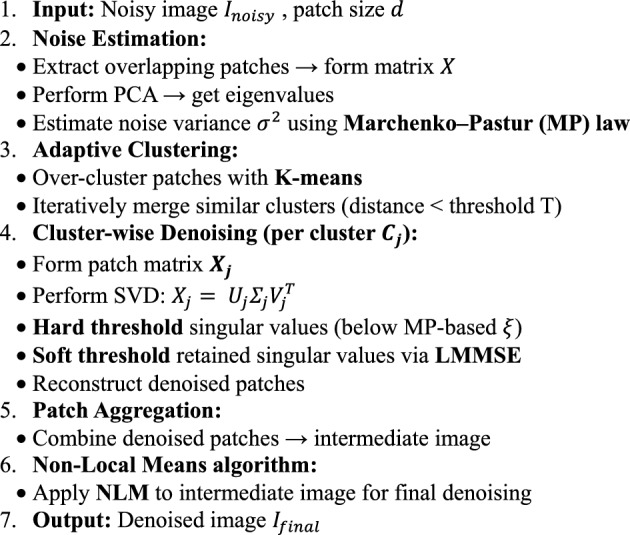
Adaptive clustering and non-local means denoising

Experimental setup and results

In the experiments, the MRI and CT image datasets were obtained from https://www.med.harvard.edu/aanlib/home.html⁴⁹, a publicly available repository of medical images for research purposes. The datasets were pre-processed by dividing them into training and testing sets to ensure robust evaluation of the denoising performance. Specifically, 70% of the images were randomly selected for training, allowing the model to learn from a diverse set of anatomical structures and noise patterns, while the remaining 30% were reserved for testing to evaluate the generalization capability of the proposed method. Both sets included images with varying noise levels (σ ≈ 10, 20, 30, 40) to simulate realistic noise conditions. Each image was divided into overlapping patches of size 8 × 8 for noise reduction and 10 × 10 for noise level estimation as described in the experimental methodology. The split ensured no overlap of image instances between training and testing to avoid data leakage. Performance was evaluated using standard metrics (PSNR, SSIM, FSIM, Entropy, BRISQUE, PIQE, NIQE) to quantify denoising quality across both sets. The quality of the image is better when PSNR^50,51, SSIM, FSIM^50,51 and Entropy have higher values, whereas BRISQU⁵², PIQE, and NIQE⁵³ should have lower values. The quantitative study confirms that the proposed noise level estimation achieves superior denoising performance on average compared to other approaches. For calculating the efficiency of the image denoising method, we compare the proposed approach with several other popular algorithms, namely OD-CNN⁵⁴, NDiff³⁰, SDPM³⁴, UDLF⁵⁵, NGN⁵⁶, CNCL⁵⁷,BP-MEC²⁵, FDCT⁵⁸, NSCT-BT⁵⁹, IDM-PM⁶⁰, ONLM⁶¹, DCT-ACO⁷, ANLM⁶², Z-NLM⁶³. Three test images with values of 10, 20, 30, and 40 are utilized for representation: two MRI images (MRI1 and MRI2) and one CT image from https://www.med.harvard.edu/aanlib/home.html⁴⁹. All these methods are configured to their default parameters for optimal performance. All experiments were conducted on a desktop computer with an Intel Core i5-4460 Quad-Core CPU running at 3.2 GHz, 16 GB of RAM, and using MATLAB R2020b as the software platform. The comparative methods were evaluated using publicly available implementations where accessible, or re-implemented according to the algorithms described in the respective publications when source code was not provided.

The ability to preserve image details is demonstrated using visual analysis in Figs. (2, 3, 4, 5, 6, 7, 8, 9, 10, 11, 12, 13) for three images at different noise levels. We begin by presenting the visual results and then present the quantitative analysis using several performance metrics. Figures (2, 3, 4) illustrates the denoising results. We introduce several degrees of Gaussian noise ( 10, 20, 30,40) to the ground truth image and implement different techniques for denoising. Figures 2, 3, 4b–c illustrates that OD-CNN and NDiff preserve the external details while the inside details are pixelated. In Figs. 2, 3, 4d–e, the SDPM and NGN approaches preserve the outer margins while the inside details remain pixelated. Figures 2, 3, 4f, g, h demonstrates that UDLF, CNCL, and BP-MEC effectively maintain the edges to some degree; nevertheless, the inside details remain indistinct. Figures 2, 3, 4k, l, m illustrates that the IDM-PM, DCT-ACO, and ANLM approaches are also ineffective in preserving the edges of the images. In Figs. 2, 3, 4b–c, it is obvious that OD-CNN and NDiff preserve the outer edges although the inner features of the image appear blurred. Figures 2, 3, 4i, j illustrates that FDCT and NSCT-BT fail to preserve edge sharpness which results in distortion. Figures 2, 3, 4n, o illustrates that Z-NLM and ONLM distort the image which results in an increased edge width. Figures 2, 3, 4p illustrates that the image generated using proposed method closely resembles the ground truth image while maintaining both internal and external details. Table 1 displays the quantitative evaluation which demonstrated computed values of PSNR, SSIM, FSIM, Entropy, BRISQUE, PIQE, and NIQE for an estimated denoised image derived from the use of several techniques across diverse noise levels in imaging. The Entropy, PSNR, FSIM, and SSIM of the denoising image produced by the proposed method are superior to those of existing techniques and PIQE, NIQE, and BRISQUE values are comparatively lower which is optimal. Figures (5, 6, 7) presents the qualitative results of the MRI2 image. Figures 5, 6, 7b, c demonstrate that the results of OD-CNN and NDiff exhibit pixelation. Figures 5, 6, 7d, e illustrate the results of the SDPM and NGN methodologies wherein the edges remain unclear and pixelated. Figures 5, 6, 7f, g, h illustrates the outputs of UDLF, CNCL, and BP-MEC, while the complex details are absent. In Figs. 5, 6, 7k, l, m, IDM-PM, DCT-ACO, and ANLM are used for image denoising which results in less clear edges that reduce the visual quality of the image. Figures 5, 6, 7b, c presents the outcomes achieved by the OD-CNN and NDiff methodologies which reveals that the outer edges are clear but the inside details are blurred. Figures 5–7i, j illustrates the results achieved by FDCT and NSCT-BT which reveals that the edges lack clarity and noise persists in the image, hence reduces its visual quality. Figures 5, 6, 7n, o illustrates that the images produced by the Z-NLM and ONLM methods exhibit blurriness and average visual quality. Figures 5, 6, 7p illustrates the findings derived from the proposed methodology which demonstrates that our model effectively minimizes noise to a greater degree than comparative methods. Table 2 lists average error scores achieved by several methodologies on the MRI2 image. The table indicates that the proposed method has superior values in Entropy, PSNR, FSIM, and SSIM compared to other methods. The proposed strategy exhibits lower PIQE, NIQE, and BRISQUE values in comparison to alternative methods which is optimal. Figures (8, 9, 10) illustrates the qualitative results of the denoised image reconstructed using several denoising techniques used in CT image affected by Gaussian noise. In Figs. 8, 9, 10b, c, OD-CNN and NDiff preserve the image structure; however, the emergence of.

Fig. 2.

Denoising results of the MRI1 image (; (a) Reference image, (b) ONLM, (c) Z-NLM, (d) ANLM, (e) DCT-ACO, (f) IDM-PM, (g) NSCT-BT, (h) FDCT, (i) BP-MEC, (j) CNCL, (k) UDLF, (l) NGN, (m) SDPM, (n) NDiff, (o) OD-CNN, and (p) Ours.

Fig. 3.

Denoising results of the MRI2 image (; (a) Reference image, (b) ONLM, (c) Z-NLM, (d) ANLM, (e) DCT-ACO, (f) IDM-PM, (g) NSCT-BT, (h) FDCT, (i) BP-MEC, (j) CNCL, (k) UDLF, (l) NGN, (m) SDPM, (n) NDiff, (o) OD-CNN, and (p) ours.

Fig. 4.

Denoising results of the CT image (; (a) Reference image, (b) ONLM, (c) Z-NLM, (d) ANLM, (e) DCT-ACO, (f) IDM-PM, (g) NSCT-BT, (h) FDCT, (i) BP-MEC, (j) CNCL, (k) UDLF, (l) NGN, (m) SDPM, (n) NDiff, (o) OD-CNN, and (p) ours.

Fig. 5.

Denoising results of the MRI1 image (; (a) Reference image, (b) ONLM, (c) Z-NLM, (d) ANLM, (e) DCT-ACO, (f) IDM-PM, (g) NSCT-BT, (h) FDCT, (i) BP-MEC, (j) CNCL, (k) UDLF, (l) NGN, (m) SDPM, (n) NDiff, (o) OD-CNN, and (p) ours.

Fig. 6.

Denoising results of the MRI2 image (; (a) Reference image, (b) ONLM, (c) Z-NLM, (d) ANLM, (e) DCT-ACO, (f) IDM-PM, (g) NSCT-BT, (h) FDCT, (i) BP-MEC, (j) CNCL, (k) UDLF, (l) NGN, (m) SDPM, (n) NDiff, (o) OD-CNN, and (p) ours.

Fig. 7.

Denoising results of the CT image (; (a) Reference image, (b) ONLM, (c) Z-NLM, (d) ANLM, (e) DCT-ACO, (f) IDM-PM, (g) NSCT-BT, (h) FDCT, (i) BP-MEC, (j) CNCL, (k) UDLF, (l) NGN, (m) SDPM, (n) NDiff, (o) OD-CNN, and (p) Ours.

Fig. 8.

Denoising results of the MRI1 image (; (a) Reference image, (b) ONLM, (c) Z-NLM, (d) ANLM, (e) DCT-ACO, (f) IDM-PM, (g) NSCT-BT, (h) FDCT, (i) BP-MEC, (j) CNCL, (k) UDLF, (l) NGN, (m) SDPM, (n) NDiff, (o) OD-CNN, and (p) ours.

Fig. 9.

Denoising results of the MRI2 image (; (a) Reference image, (b) ONLM, (c) Z-NLM, (d) ANLM, (e) DCT-ACO, (f) IDM-PM, (g) NSCT-BT, (h) FDCT, (i) BP-MEC, (j) CNCL, (k) UDLF, (l) NGN, (m) SDPM, (n) NDiff, (o) OD-CNN, and (p) ours.

Fig. 10.

Denoising results of the CT image (; (a) Reference image, (b) ONLM, (c) Z-NLM, (d) ANLM, (e) DCT-ACO, (f) IDM-PM, (g) NSCT-BT, (h) FDCT, (i) BP-MEC, (j) CNCL, (k) UDLF, (l) NGN, (m) SDPM, (n) NDiff, (o) OD-CNN, and (p) ours.

Fig. 11.

Denoising results of the MRI1 image (; (a) Reference image, (b) ONLM, (c) Z-NLM, (d) ANLM, (e) DCT-ACO, (f) IDM-PM, (g) NSCT-BT, (h) FDCT, (i) BP-MEC, (j) CNCL, (k) UDLF, (l) NGN, (m) SDPM, (n) NDiff, (o) OD-CNN, and (p) ours.

Fig. 12.

Denoising results of the MRI2 image (; (a) Reference image, (b) ONLM, (c) Z-NLM, (d) ANLM, (e) DCT-ACO, (f) IDM-PM, (g) NSCT-BT, (h) FDCT, (i) BP-MEC, (j) CNCL, (k) UDLF, (l) NGN, (m) SDPM, (n) NDiff, (o) OD-CNN, and (p) ours.

Fig. 13.

Denoising results of the MRI2 image (; (a) Reference image, (b) ONLM, (c) Z-NLM, (d) ANLM, (e) DCT-ACO, (f) IDM-PM, (g) NSCT-BT, (h) FDCT, (i) BP-MEC, (j) CNCL, (k) UDLF, (l) NGN, (m) SDPM, (n) NDiff, (o) OD-CNN, and (p) Ours.

Table 1.

The performance of different denoising algorithms is evaluated based on Entropy, PSNR, SSIM, FSIM, BRISQUE, PIQE and NIQE metrics for MRI1 image.

Method	σ	Entropy	PSNR	SSIM	FSIM	BRISQUE	NIQE	PIQE
Ours	10	6.70	34.97	0.94	0.95	43.22	5.13	56.44
	20	6.69	31.79	0.90	0.92	46.04	4.78	61.16
	30	6.73	29.80	0.86	0.90	44.28	4.69	56.74
	40	6.87	28.38	0.82	0.87	43.58	5.13	54.41
OD-CNN	10	6.45	32.29	0.93	0.88	43.82	5.88	60.41
	20	6.08	27.97	0.88	0.87	48.14	5.42	51.24
	30	6.10	26.37	0.83	0.86	47.90	5.92	43.01
	40	6.16	23.87	0.81	0.85	46.12	5.49	37.10
NDiff	10	5.78	30.76	0.89	0.88	44.38	5.22	51.83
	20	5.87	24.99	0.82	0.86	46.38	5.56	43.28
	30	5.86	22.67	0.83	0.89	45.24	5.44	43.59
	40	5.47	26.86	0.80	0.83	47.46	5.67	69.45
SDPM	10	5.42	28.75	0.87	0.84	47.12	5.36	57.85
	20	5.69	25.35	0.83	0.86	49.66	4.90	74.79
	30	5.68	22.86	0.83	0.83	48.16	5.29	77.64
	40	5.98	20.31	0.82	0.81	48.46	5.38	84.50
NGN	10	5.64	27.64	0.83	0.86	51.19	5.39	42.50
	20	5.84	25.52	0.79	0.83	55.29	5.65	59.84
	30	5.70	24.89	0.77	0.79	48.81	4.83	53.07
	40	5.96	21.94	0.79	0.79	53.70	5.84	73.97
UDLF	10	5.20	26.25	0.85	0.81	50.79	5.49	24.58
	20	5.42	23.21	0.80	0.78	51.56	5.67	19.98
	30	5.45	21.08	0.81	0.79	52.53	5.57	19.55
	40	5.32	15.86	0.78	0.73	53.43	6.01	20.89
CNCL	10	6.04	26.39	0.80	0.83	53.63	5.93	70.09
	20	5.14	23.70	0.79	0.75	50.77	5.11	61.51
	30	5.24	22.27	0.76	0.77	49.31	4.92	56.82
	40	5.87	17.39	0.77	0.73	54.25	6.48	39.88
BP-MEC	10	5.69	27.04	0.79	0.82	52.67	5.83	45.29
	20	5.91	23.17	0.78	0.78	58.86	6.53	58.31
	30	5.97	21.21	0.77	0.77	53.18	6.07	62.54
	40	5.71	16.91	0.78	0.78	53.46	5.56	77.20
FDCT	10	5.89	26.02	0.76	0.79	50.59	6.16	32.45
	20	5.05	22.69	0.75	0.76	54.79	5.86	31.28
	30	5.10	22.31	0.71	0.73	57.77	6.13	37.72
	40	5.14	16.13	0.70	0.76	53.85	6.60	63.32
NSCT-BT	10	5.47	25.92	0.75	0.77	51.22	6.67	33.98
	20	5.23	23.18	0.73	0.75	52.89	6.87	34.67
	30	5.08	22.98	0.71	0.73	53.45	6.98	35.67
	40	4.98	21.89	0.69	0.71	55.72	7.10	36.77
IDM-PM	10	5.25	24.98	0.73	0.74	52.85	6.65	36.98
	20	5.12	23.88	0.71	0.73	53.16	6.78	37.45
	30	4.97	22.17	0.69	0.70	54.95	6.89	37.98
	40	4.78	20.78	0.67	0.68	55.17	6.99	38.17
DCT-ACO	10	4.61	24.93	0.71	0.77	54.73	6.68	42.56
	20	4.87	21.60	0.66	0.73	58.42	6.62	53.45
	30	4.82	21.73	0.69	0.76	56.32	6.56	60.74
	40	4.93	15.53	0.68	0.73	53.46	6.90	79.95
ANLM	10	4.57	23.28	0.69	0.75	55.17	6.67	40.67
	20	4.43	22.19	0.67	0.73	55.67	6.88	42.82
	30	4.10	20.98	0.65	0.69	56.19	6.89	43.92
	40	4.56	19.83	0.63	0.67	57.14	7.06	44.77
Z-NLM	10	4.35	23.99	0.69	0.76	55.67	6.87	38.78
	20	4.27	22.19	0.67	0.73	57.88	6.89	39.78
	30	4.05	20.89	0.65	0.69	58.34	7.10	40.18
	40	4.02	18.28	0.63	0.66	59.11	7.23	42.66
ONLM	10	4.27	22.89	0.67	0.73	56.87	6.93	39.97
	20	4.10	21.29	0.65	0.69	57.89	7.04	41.29
	30	3.97	19.98	0.64	0.67	58.17	7.17	42.77
	40	3.83	18.66	0.62	0.64	59.66	7.27	44.87

The best performing results are highlighted in bold for clarity.

Table 2.

The performance of different denoising algorithms is evaluated based on Entropy, PSNR, SSIM, FSIM, BRISQUE, PIQE and NIQE metrics for MRI2 image.

Method	σ	Entropy	PSNR	SSIM	FSIM	BRISQUE	NIQE	PIQE
Ours	10	6.34	35.58	0.95	0.96	48.07	5.25	55.52
	20	6.36	32.35	0.90	0.93	48.93	4.73	54.53
	30	6.44	30.28	0.86	0.90	44.63	4.72	51.40
	40	6.60	28.64	0.80	0.88	36.57	4.35	53.91
OD-CNN	10	6.12	34.72	0.88	0.93	49.74	5.67	57.01
	20	6.01	31.10	0.86	0.92	49.53	5.59	59.32
	30	6.14	29.38	0.81	0.89	46.98	5.74	56.77
	40	6.13	27.18	0.78	0.87	47.52	5.97	58.78
NDiff	10	5.34	32.06	0.84	0.92	53.50	5.65	60.68
	20	5.43	26.08	0.80	0.87	55.02	5.30	63.42
	30	5.44	26.98	0.79	0.86	53.45	5.83	58.80
	40	5.19	28.22	0.80	0.88	53.46	5.71	60.93
SDPM	10	5.99	28.28	0.81	0.89	53.01	5.78	64.14
	20	6.22	26.45	0.77	0.87	48.43	5.88	64.74
	30	5.24	23.85	0.74	0.86	54.17	5.99	68.09
	40	5.82	23.65	0.81	0.85	45.46	6.14	65.00
NGN	10	6.15	26.98	0.76	0.88	54.74	6.21	59.31
	20	5.29	23.25	0.72	0.86	52.91	6.00	57.90
	30	6.06	23.06	0.75	0.86	62.16	5.96	60.30
	40	5.44	20.16	0.72	0.84	53.51	5.54	64.00
UDLF	10	5.81	30.11	0.85	0.86	50.93	5.79	65.64
	20	6.00	23.91	0.81	0.82	62.60	5.74	60.67
	30	6.06	21.83	0.76	0.81	63.19	6.10	58.74
	40	6.17	21.60	0.73	0.80	53.43	5.80	59.80
CNCL	10	5.58	29.98	0.84	0.78	49.36	5.84	62.39
	20	5.71	25.60	0.81	0. 77	50.44	6.28	65.95
	30	5.75	23.82	0.76	0.77	59.54	5.69	62.60
	40	5.62	18.56	0.73	0.76	54.46	6.50	64.01
BP-MEC	10	5.33	30.64	0.83	0.84	59.14	5.77	63.71
	20	5.49	24.94	0.79	0.82	63.42	5.99	62.22
	30	5.51	23.20	0.75	0.79	63.46	6.19	65.91
	40	5.40	18.23	0.70	0.78	53.49	6.04	66.40
FDCT	10	5.46	29.27	0.79	0.77	60.18	6.15	66.57
	20	5.63	25.60	0.75	0.78	59.60	6.79	67.40
	30	5.69	23.48	0.80	0.73	60.89	6.99	69.31
	40	4.88	19.09	0.76	0.81	63.49	6.74	71.55
NSCT-BT	10	5.42	27.89	0.78	0.75	61.99	6.87	67.19
	20	5.27	25.19	0.73	0.73	62.88	6.98	68.99
	30	5.10	24.81	0.71	0.71	63.89	7.10	70.01
	40	5.03	23.78	0.68	0.69	64.64	7.23	72.22
IDM-PM	10	5.27	26.99	0.76	0.77	62.87	6.93	68.83
	20	5.13	25.81	0.73	0.75	63.99	7.04	69.87
	30	4.98	24.67	0.71	0.73	65.78	7.15	71.88
	40	4.78	22.18	0.69	0.71	66.16	7.20	72.99
DCT-ACO	10	5.06	27.18	0.75	0.79	64.95	6.70	67.74
	20	5.20	23.84	0.74	0.76	59.45	6.99	68.57
	30	5.23	21.99	0.76	0.73	57.12	6.81	74.56
	40	4.62	16.78	0.69	0.70	60.42	7.64	69.08
ANLM	10	4.98	26.93	0.74	0.78	65.89	6.74	67.99
	20	4.79	25.17	0.73	0.75	66.67	6.87	69.89
	30	4.66	23.89	0.71	0.74	69.18	7.01	71.72
	40	4.56	22.19	0.67	0.73	70.18	7.17	72.89
Z-NLM	10	4.87	25.66	0.73	0.77	65.67	6.99	69.99
	20	4.67	23.89	0.69	0.76	66.18	7.23	70.99
	30	4.56	22.29	0.67	0.74	67.78	7.27	71.87
	40	4.23	21.87	0.65	0.71	69.89	7.32	72.19
ONLM	10	4.67	24.89	0.69	0.74	66.98	7.17	70.67
	20	4.45	23.28	0.67	0.72	70.18	7.20	72.89
	30	4.26	22.95	0.64	0.69	71.35	7.25	73.29
	40	4.10	21.89	0.62	0.67	72.97	7.29	74.88

The best performing results are highlighted in bold for clarity.

grainy formations result in unclear edges. Figures 8, 9, 10d, e demonstrates that SDPM and NGN alleviate noise to a certain extent; however, the structure is slightly shifted from its original position. Figures 8, 9, 10f, g, h demonstrates that UDLF, CNCL, and BP-MEC fail to smooth the homogenous zones which results in a fragmented appearance. In Figs. 8–10k, l, m, we note that the outputs of IDM-PM, DCT-ACO, and ANLM are unclear which makes it difficult to distinguish the borders. Figures 8–10b, d demonstrates that overall, noise reduction is achieved by the OD-CNN and NDiff approaches; nevertheless, finer details could be enhanced. Figures 8, 9, 10i, j displays the denoised outputs from FDCT and NSCT-BT whereby noise remains visible. Figures 8, 9, 10n, o illustrates that Z-NLM and ONLM unclear the image, hence reduces its visual quality. Figures 8, 9, 10p demonstrates the result obtained from the proposed methodology that reveals that the reconstructed image closely resembles the ground truth image. The result obtained from the proposed approach for image denoising reduces.

the noise level to some degree. Table 3 presents the quantitative findings of all methods across various noise levels, indicating that the Entropy, PSNR, FSIM, and SSIM scores of the proposed approach surpass those of other methods while the PIQE, NIQE, and BRISQUE values of the proposed approach are comparatively low. We note that IDM-PM, DCT-ACO, and ANLM fails to preserve the edges, where interpreting boundary differentiation impossible. SDPM and NGN preserve the edges; nonetheless, noise remains in the image. The result indicates that the structure is preserved by UDLF, CNCL, and BP-MEC; nevertheless, the details in the image are compromised. The image produced by utilizing IDM-PM, DCT-ACO, and ANLM algorithms on the input image fails to maintain structural integrity. SDPM and NGN effectively retain edges; nonetheless, noise persists in the homogeneous areas of the image. The image produced by FDCT and NSCT-BT remains significantly noisy. It indicates that Z-NLM and ONLM cause the image to become blurred, where interpreting any portion of the image unclear. Our method outperforms other methods while preserving edges and maintaining visual quality. The data presented in Figs. 11, 12, 13 and Tables (1, 2, 3) indicates that the proposed approach outperforms other methods. Our noise level estimation approach offers more precise and consistent assessment of noise levels in medical images compared to current leading algorithms. The proposed denoising method generates superior restoration of essential image information as compared to state-of-the-art denoising techniques. It is noticed that the hard thresholding of singular values for the non-local groups is also illustrated in⁶⁴. But our method differs from⁶⁴ by using adaptive clustering of non-local patches and a more advanced PCA thresholding using to MP law. In addition to the PCA thresholding in the initial phase, the local approximation is used in the coefficient-wise LMMSE filtering during a subsequent phase which further aids in maintaining image detail when compared with the global LMMSE. The incorporation of the non-local means (NLM) algorithm provides substantial advantages by maintaining complex details and textures while efficiently reducing noise. By leveraging the redundancy of similar pixels across the image and it ensures denoising is adaptive and data-driven while making it mostly effective for handling complex and textured regions. This leads to significantly improved visual quality compared to state-of-the-art methods particularly for images with complex details or challenging low signal-to-noise ratios.

Table 3.

The performance of different denoising algorithms is evaluated based on Entropy, PSNR, SSIM, FSIM, BRISQUE, PIQE and NIQE metrics for CT image.

Method	σ	Entropy	PSNR	SSIM	FSIM	BRISQUE	NIQE	PIQE
Ours	10	7.16	29.68	0.82	0.90	23.76	3.38	23.80
	20	7.08	27.45	0.73	0.85	28.40	3.05	25.25
	30	7.11	26.11	0.67	0.84	21.20	3.32	21.89
	40	7.09	25.10	0.62	0.82	29.81	3.60	26.76
OD-CNN	10	7.01	27.45	0.79	0.85	25.90	4.16	29.99
	20	7.00	23.67	0.73	0.81	25.87	4.13	27.70
	30	6.95	21.80	0.66	0.80	26.37	4.84	26.10
	40	6.56	20.02	0.61	0.78	30.78	5.10	28.15
NDiff	10	6.14	25.25	0.72	0.83	31.94	4.61	30.76
	20	6.71	21.76	0.69	0.82	32.30	4.30	29.44
	30	6.75	20.15	0.63	0.79	32.74	4.06	28.23
	40	6.62	19.09	0.59	0.76	33.46	4.36	35.30
SDPM	10	6.70	23.19	0.69	0.81	30.60	3.66	34.15
	20	6.88	22.55	0.63	0.78	30.08	4.19	31.32
	30	6.78	21.11	0.60	0.77	36.09	5.12	30.27
	40	6.00	18.07	0.57	0.73	33.46	4.40	31.27
NGN	10	6.33	25.72	0.73	0.80	30.60	4.96	35.65
	20	6.99	22.76	0.58	0.79	30.91	5.42	38.58
	30	6.49	23.34	0.58	0.77	33.56	4.74	44.13
	40	6.19	19.69	0.55	0.76	36.37	4.60	33.72
UDLF	10	6.34	23.49	0.67	0.71	37.29	5.42	37.71
	20	5.51	20.96	0.59	0.78	35.28	5.65	42.64
	30	5.58	19.31	0.53	0.78	42.83	5.07	41.62
	40	5.52	14.05	0.54	0.76	43.38	5.30	35.04
CNCL	10	6.17	23.51	0.62	0.79	41.31	5.24	40.60
	20	6.22	21.67	0.60	0.73	43.54	5.14	43.77
	30	6.23	20.90	0.59	0.72	42.93	5.54	48.53
	40	6.05	18.75	0.51	0.73	35.23	4.98	43.25
BP-MEC	10	5.97	24.31	0.65	0.74	37.55	4.24	47.41
	20	5.87	21.50	0.51	0.71	42.83	5.22	52.59
	30	5.93	19.85	0.55	0.69	43.44	5.55	46.08
	40	5.87	14.41	0.50	0.68	43.46	5.52	55.69
FDCT	10	5.19	23.37	0.66	0.79	34.16	6.05	55.86
	20	6.07	22.06	0.58	0.76	43.93	6.20	49.63
	30	5.10	20.30	0.52	0.72	37.64	6.69	48.81
	40	5.31	14.26	0.56	0.70	43.78	5.90	54.93
NSCT-BT	10	5.03	22.89	0.65	0.77	35.89	6.27	56.89
	20	4.93	21.28	0.64	0.75	36.78	6.55	57.19
	30	4.67	20.98	0.63	0.73	37.89	6.67	58.99
	40	4.55	19.27	0.61	0.71	38.18	6.83	59.18
IDM-PM	10	4.97	22.67	0.63	0.76	36.88	6.34	57.19
	20	4.87	21.22	0.62	0.74	37.88	6.55	58.99
	30	4.73	20.19	0.59	0.72	38.18	6.66	59.17
	40	4.66	18.97	0.57	0.71	39.99	6.89	61.83
DCT-ACO	10	5.13	22.08	0.64	0.77	36.42	6.33	58.37
	20	5.06	21.06	0.50	0.75	40.83	7.09	61.89
	30	4.66	20.15	0.47	0.69	46.99	5.68	53.12
	40	4.14	13.77	0.54	0.66	43.49	6.92	59.15
ANLM	10	4.92	21.78	0.62	0.75	36.78	6.45	59.99
	20	4.68	20.91	0.59	0.73	37.88	6.78	60.98
	30	4.55	19.88	0.56	0.70	38.18	6.87	61.25
	40	4.47	18.99	0.53	0.69	39.67	6.98	62.35
Z-NLM	10	4.67	21.87	0.61	0.74	37.11	6.67	59.17
	20	4.45	20.90	0.58	0.71	38.98	6.76	60.19
	30	4.29	18.99	0.55	0.68	40.18	6.88	61.77
	40	4.27	17.97	0.53	0.65	41.87	6.95	62.56
ONLM	10	4.55	20.89	0.59	0.73	38.18	6.83	61.38
	20	4.41	19.28	0.57	0.71	39.18	6.89	62.18
	30	4.26	18.26	0.52	0.69	40.89	6.94	63.89
	40	4.22	17.16	0.50	0.67	41.87	7.01	64.78

Ablation study

To validate the effectiveness of outlier exclusion and smoothing within the adaptive clustering and denoising process, we performed an ablation study to quantify their individual contributions to overall denoising performance. Specifically, we compared the full proposed method against two reduced variants: (1) a version without the iterative merging phase of adaptive clustering (thereby reducing outlier exclusion), and (2) a version omitting the soft thresholding (smoothing) step based on LMMSE. The evaluation was performed using MRI and CT datasets from the Cancer Imaging Archive under Gaussian noise levels σ = 10, 20, 30, and 40.

We used PSNR, SSIM, FSIM, Entropy, BRISQUE, NIQE, and PIQE as performance metrics. The quantitative results are presented in Table 4. The results show that excluding the merging phase reduced PSNR by an average of 1.2 dB and SSIM by 0.03 across noise levels, indicating the importance of outlier exclusion in preserving structural similarity. Similarly, omitting the LMMSE-based soft thresholding reduced PSNR by 0.8 dB and SSIM by 0.02, while slightly increasing BRISQUE, NIQE, and PIQE scores. These findings demonstrate that both strategies synergistically enhance the method’s denoising effectiveness by balancing noise suppression and detail preservation. Figure 14 presents a comprehensive comparison of quantitative evaluation metrics such as PSNR, SSIM, FSIM, Entropy, BRISQUE, and PIQE across different noise levels ( = 10, 20, 30, 40) for the proposed method, a variant without the merging phase (no merging), and a variant without the soft thresholding step (no soft thresholding). The results clearly demonstrate that the proposed method consistently outperforms both ablated variants across all metrics and noise levels. Specifically, the proposed method achieves the highest PSNR, SSIM, and FSIM values, indicating superior noise suppression, structural similarity preservation, and feature similarity retention, respectively. In contrast, the no merging and no soft thresholding variants exhibit a noticeable degradation in performance, particularly at higher noise levels. Similarly, the proposed method yields lower BRISQUE, PIQE and NIQE scores across noise levels, signifying improved perceptual quality compared to the ablated variants. The entropy values also suggest that the proposed method better maintains image detail while suppressing noise. These findings collectively validate the individual and combined contributions of the merging phase (outlier exclusion) and the soft thresholding step in enhancing the overall denoising effectiveness of the proposed approach.

Table 4.

Ablation study results showing the effect of outlier exclusion and soft thresholding on denoising metrics at varying noise levels.

Noise level (σ)	Method	PSNR	SSIM	FSIM	Entropy	BRISQUE	NIQE	PIQE
10	Proposed	34.97	0.94	0.95	6.7	43.22	5.13	56.44
10	No merging	33.7	0.91	0.93	6.65	46.85	5.45	58.21
10	No soft thresholding	34.1	0.92	0.94	6.68	45.32	5.28	57.49
20	Proposed	31.79	0.9	0.92	6.69	46.04	4.78	61.16
20	No merging	30.55	0.87	0.9	6.63	48.7	5.05	62.89
20	No soft thresholding	30.92	0.88	0.91	6.66	47.29	4.95	62.1
30	Proposed	29.8	0.86	0.9	6.73	44.28	4.69	56.74
30	No merging	28.52	0.83	0.88	6.68	46.92	4.92	58.1
30	No soft thresholding	28.95	0.84	0.89	6.71	45.88	4.79	57.53
40	Proposed	28.38	0.82	0.87	6.87	43.58	5.13	54.41
40	No merging	27.05	0.79	0.85	6.8	46.11	5.29	55.96
40	No soft thresholding	27.53	0.8	0.86	6.84	44.96	5.2	55.12

Fig. 14.

Quantitative metric comparisons (PSNR, SSIM, FSIM, Entropy, BRISQUE, PIQE, NIQE) for the ablation study across noise levels (σ = 10, 20, 30, 40), comparing the proposed method, no merging variant, and no soft thresholding variant.

In order to evaluate the computational efficiency of the proposed method under varying noise conditions, we measured the average running time at different noise standard deviations ( = 10, 20, 30, 40) across MRI1, MRI2, and CT images. The results, previously presented in Table 3, were further visualized in a running time versus noise level curve (see Fig. 15) to facilitate a clearer comparative interpretation. This figure demonstrates that while the running time slightly increases with noise density, the increase is relatively modest and remains computationally feasible within clinical and research settings. Additionally, the proposed method maintains a favourable balance between running time and denoising performance, especially at higher noise levels, outperforming several benchmark methods in robustness despite a moderate increase in execution time. This visualization confirms that the scalability of the method with respect to noise level is practically acceptable.

Fig. 15.

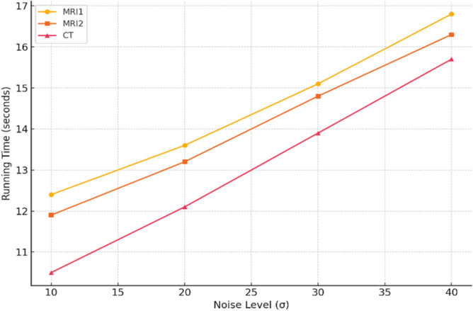
Running time (in seconds) vs. noise level ( = 10, 20, 30, 40) for MRI1, MRI2, and CT images.

Conclusion

This study proposes a robust noise level estimation method along with a cluster-wise denoising approach. Our noise level estimation approach is more precise and reliable for medical images compared to other methods. The proposed denoising method uses an adaptive clustering method to employ effectively grouping nonlocal patches based on their special features. Each cluster is then accurately denoised using a PCA thresholding strategy. The denoising process begins with the removal of the most of noise through an enhanced singular value hard thresholding system based on MP law. This is followed by further refinement of noise reduction using coefficient-wise PCA domain LMMSE filtering which is a specific method of soft thresholding with locally computed parameters. Our method delivers superior detail preservation and outperforms other comparative methods in image denoising by combining denoising frameworks with an adaptive clustering method. Besides, the NL-Means algorithm reduces noise by estimating weighted averages of the pixels using the similarity of patches. It evaluates patch similarity using a Gaussian-weighted Euclidean distance which ensures further effective noise suppression while preserving textures and structures. Our future work will focus on enhancing the proposed approach and exploring its applications in other medical imaging and computer vision. In particular, we aim to improve image restoration techniques to address noise and alleviate any degradation in medical imagery by ensuring higher accuracy and reliability in clinical applications.

Author contributions

M.S.: conceptualization, data analysis, experimental design, execution, and original draft preparation. A.D.: methodology, experimental design, project administration, validation, and original draft preparation. B.G.: conceptualization, experimental design, execution, and original draft preparation. A.G.: methodology, experimental design, and original draft preparation. M.J.S.: investigation, validation, supervision, funding acquisition, review and final manuscript preparation. All authors have read and approved the manuscript.

Data availability

The datasets used in this study are openly available on (1) The Whole Brain ATLAS, https://www.med.harvard.edu/aanlib/home.html and (2) Image-Fusion-Image-Denoising-Image-Enhancement, https://github.com/Imagingscience/Image-Fusion-Image-Denoising-Image-Enhancement-

Declarations

Competing interests

The authors declare no competing interests.

References

- 1.Nazir, N., Sarwar, A. & Saini, B. S. Recent developments in denoising medical images using deep learning: An overview of models, techniques, and challenges. Micron180, 103615. 10.1016/J.MICRON.2024.103615 (2024). [DOI] [PubMed] [Google Scholar]
- 2.El-Shafai, W., El-Nabi, S. A., Ali, A. M., El-Rabaie, E. S. M. & Abd El-Samie, F. E. Traditional and deep-learning-based denoising methods for medical images. Multimed. Tools Appl.83(17), 52061–52088. 10.1007/S11042-023-14328-X/METRICS (2024). [Google Scholar]
- 3.Jifara, W., Jiang, F., Rho, S., Cheng, M. & Liu, S. Medical image denoising using convolutional neural network: A residual learning approach. J. Supercomput.75(2), 704–718. 10.1007/S11227-017-2080-0/METRICS (2019). [Google Scholar]
- 4.Binh, N. T. & Khare, A. Adaptive complex wavelet technique for medical image denoising. IFMBE Proc.27, 196–199. 10.1007/978-3-642-12020-6_49 (2010). [Google Scholar]
- 5.Satapathy, L. M., Das, P., Shatapathy, A. & Patel, A. Bio-medical image denoising using wavelet transform. Int. J. Recent Technol. Eng8(1), 2874–2879 (2019). [Google Scholar]
- 6.Bai, J., Song, S., Fan, T. & Jiao, L. Medical image denoising based on sparse dictionary learning and cluster ensemble. Soft. Comput.22(5), 1467–1473. 10.1007/S00500-017-2853-7/METRICS (2018). [Google Scholar]
- 7.Miri, A., Sharifian, S., Rashidi, S. & Ghods, M. Medical image denoising based on 2D discrete cosine transform via ant colony optimization. Optik (Stuttg)156, 938–948. 10.1016/J.IJLEO.2017.12.074 (2018). [Google Scholar]
- 8.Chithra, R. S. & Jagatheeswari, P. Enhanced WOA and modular neural network for severity analysis of tuberculosis. Multimed. Res.10.46253/J.MR.V2I3.A5 (2019). [Google Scholar]
- 9.Do, M. N. & Vetterli, M. The contourlet transform: An efficient directional multiresolution image representation. IEEE Trans. Image Process.14(12), 2091–2106. 10.1109/TIP.2005.859376 (2005). [DOI] [PubMed] [Google Scholar]
- 10.Marčenko, V. A. & Pastur, L. A. Distribution of eigenvalues for some sets of random matrices. Math. USSR-Sbornik1(4), 457–483. 10.1070/SM1967V001N04ABEH001994 (1967). [Google Scholar]
- 11.Veraart, J., Fieremans, E. & Novikov, D. S. Diffusion MRI noise mapping using random matrix theory. Magn. Reson. Med.76(5), 1582–1593. 10.1002/MRM.26059 (2016). [DOI] [PMC free article] [PubMed] [Google Scholar]
- 12.Veraart, J. et al. Denoising of diffusion MRI using random matrix theory. Neuroimage142, 394–406. 10.1016/J.NEUROIMAGE.2016.08.016 (2016). [DOI] [PMC free article] [PubMed] [Google Scholar]
- 13.Ike, C. S., Muhammad, N., Bibi, N., Alhazmi, S. & Eoghan, F. Discriminative context-aware network for camouflaged object detection. Front. Artif. Intell.10.3389/frai.2024.1347898 (2024). [DOI] [PMC free article] [PubMed] [Google Scholar]
- 14.Khan, H., Xiao, B., Li, W. & Muhammad, N. Recent advancement in haze removal approaches. Multimed. Syst.28, 687–710. 10.1007/s00530-021-00865-8 (2022). [Google Scholar]
- 15.Muhammad, N. et al. Frequency component vectorisation for image dehazing. J. Exper. Theor. Artif. Intell.10.1080/0952813X.2020.1794232 (2020). [Google Scholar]
- 16.Ike, C. S. & Muhammad, N. Separable property-based super-resolution of lousy image data. Pattern Anal. Appl.23, 1407–1420. 10.1007/s10044-019-00854-8 (2020). [Google Scholar]
- 17.Khan, H. et al. Localization of radiance transformation for image dehazing in wavelet domain. Neurocomputing381, 141–151. 10.1016/j.neucom.2019.10.005 (2020). [Google Scholar]
- 18.Khan, S. N. et al. Early CU depth decision and reference picture selection for low complexity MV-HEVC. Symmetry (Basel)10.3390/sym11040454 (2019). [Google Scholar]
- 19.Muhammad, N. et al. Image noise reduction based on block matching in wavelet frame domain. Multimed. Tools Appl.79, 26327–26344. 10.1007/s11042-020-09158-0 (2020). [Google Scholar]
- 20.Muhammad, N., Bibi, N., Jahangir, A. & Mahmood, Z. Image denoising with norm weighted fusion estimators. Pattern Anal. Appl.21, 1013–1022. 10.1007/s10044-017-0617-8 (2018). [Google Scholar]
- 21.Muhammad, N. et al. Image de-noising with subband replacement and fusion process using bayes estimators. Comput. Electr. Eng.70, 413–427. 10.1016/j.compeleceng.2017.05.023 (2018). [Google Scholar]
- 22.Khmag, A. Natural digital image mixed noise removal using regularization Perona-Malik model and pulse coupled neural networks. Soft. Comput.27, 15523–15532. 10.1007/s00500-023-09148-y (2023). [Google Scholar]
- 23.Khmag, A. Additive Gaussian noise removal based on generative adversarial network model and semi-soft thresholding approach. Multimed. Tools Appl.82, 7757–7777. 10.1007/s11042-022-13569-6 (2023). [Google Scholar]
- 24.Khmag, A., Al Haddad, S. A. R., Ramlee, R. A., Kamarudin, N. & Malallah, F. L. Natural image noise removal using nonlocal means and hidden Markov models in transform domain. Vis. Comput.34, 1661–1675. 10.1007/s00371-017-1439-9 (2018). [Google Scholar]
- 25.Ji, L., Guo, Q. & Zhang, M. Medical image denoising based on biquadratic polynomial with minimum error constraints and low-rank approximation. IEEE Access8, 84950–84960. 10.1109/ACCESS.2020.2990463 (2020). [Google Scholar]
- 26.Aravindan, T. E., Seshasayanan, R. & Vishvaksenan, K. S. Medical image denoising by using discrete wavelet transform: Neutrosophic theory new direction. Cogn. Syst. Res.10.1016/j.cogsys.2018.10.027 (2018). [Google Scholar]
- 27.Rani M. L. P., Sasibhushana Rao G., Prabhakara Rao B. ANN application for medical image denoising. In Advances in Intelligent Systems and Computing Vol. 816 675–684 (2019). 10.1007/978-981-13-1592-3_53
- 28.Laves M. H., Tölle M., & Ortmaier T. Uncertainty estimation in medical image denoising with bayesian deep image prior. Lecture Notes in Computer Science (Including Subseries Lecture Notes in Artificial Intelligence and Lecture Notes in Bioinformatics) Vol. 12443 LNCS 81–96 (2020). 10.1007/978-3-030-60365-6_9/FIGURES/11
- 29.Vijaya, K. S. & Nagaraju, C. T2FCS filter: Type 2 fuzzy and cuckoo search-based filter design for image restoration. J. Vis. Commun. Image Represent.58, 619–641. 10.1016/J.JVCIR.2018.12.020 (2019). [Google Scholar]
- 30.Kollem, S., Reddy, K. R. & Rao, D. S. A novel diffusivity function-based image denoising for MRI medical images. Multimed. Tools Appl.82(21), 32057–32089. 10.1007/S11042-023-14457-3/METRICS (2023). [Google Scholar]
- 31.Huang, H. et al. Self-supervised medical image denoising based on WISTA-Net for human healthcare in metaverse. IEEE J. Biomed. Health Inform.10.1109/JBHI.2023.3278538 (2023). [DOI] [PubMed] [Google Scholar]
- 32.Chyophel Lepcha, D., Goyal, B. & Dogra, A. Low-dose CT image denoising using sparse 3d transformation with probabilistic non-local means for clinical applications. Imag. Sci. J.71(2), 97–109. 10.1080/13682199.2023.2176809 (2023). [Google Scholar]
- 33.Jang, S. I. et al. Spach transformer: spatial and channel-wise transformer based on local and global self-attentions for PET image denoising. IEEE Trans. Med. Imag.43(6), 2036–2049. 10.1109/TMI.2023.3336237 (2024). [DOI] [PMC free article] [PubMed] [Google Scholar]
- 34.Shen C., Yang Z., & Zhang Y. PET image denoising with score-based diffusion probabilistic models. Lecture Notes in Computer Science (including subseries Lecture Notes in Artificial Intelligence and Lecture Notes in Bioinformatics) Vol. 14220 LNCS, 270–278 (2023). 10.1007/978-3-031-43907-0_26
- 35.Lepcha, D. C. et al. A constructive non-local means algorithm for low-dose computed tomography denoising with morphological residual processing. PLoS ONE18(9), e0291911. 10.1371/JOURNAL.PONE.0291911 (2023). [DOI] [PMC free article] [PubMed] [Google Scholar]
- 36.Ma, Y. et al. StruNet: Perceptual and low-rank regularized transformer for medical image denoising. Med. Phys.50(12), 7654–7669. 10.1002/MP.16550 (2023). [DOI] [PubMed] [Google Scholar]
- 37.Annavarapu, A. & Borra, S. An adaptive watershed segmentation based medical image denoising using deep convolutional neural networks. Biomed. Signal Process. Control93, 106119. 10.1016/J.BSPC.2024.106119 (2024). [Google Scholar]
- 38.Zeng, X., Guo, Y., Li, L. & Liu, Y. Continual medical image denoising based on triplet neural networks collaboration. Comput. Biol. Med.179, 108914. 10.1016/J.COMPBIOMED.2024.108914 (2024). [DOI] [PubMed] [Google Scholar]
- 39.Sharif, S. M. A., Naqvi, R. A. & Loh, W. K. Two-stage deep denoising with self-guided noise attention for multimodal medical images. IEEE Trans. Radiat. Plasma Med. Sci.8(5), 521–531. 10.1109/TRPMS.2024.3380090 (2024). [Google Scholar]
- 40.Lee, K. et al. Multi-scale self-attention network for denoising medical images. APSIPA Trans. Signal Inf. Process.12, 204. 10.1561/116.00000169 (2024). [Google Scholar]
- 41.Hu, H. & Huang, Z. BeFOI: A novel method based on conditional diffusion model for medical image denoising. J. Electron. Res. Appl.8(2), 158–165. 10.26689/JERA.V8I2.6394 (2024). [Google Scholar]
- 42.Zhao, W., Lv, Y., Liu, Q. & Qin, B. Detail-preserving image denoising via adaptive clustering and progressive PCA thresholding. IEEE Access6, 6303–6315. 10.1109/ACCESS.2017.2780985 (2018). [Google Scholar]
- 43.Pyatykh, S., Hesser, J. & Zheng, L. Image noise level estimation by principal component analysis. IEEE Trans. Image Process.22(2), 687–699. 10.1109/TIP.2012.2221728 (2013). [DOI] [PubMed] [Google Scholar]
- 44.Liu, X., Tanaka, M. & Okutomi, M. Single-image noise level estimation for blind denoising. IEEE Trans. Image Process.22(12), 5226–5237. 10.1109/TIP.2013.2283400 (2013). [DOI] [PubMed] [Google Scholar]
- 45.Chen G., Zhu F., & Ann Heng P. An efficient statistical method for image noise level estimation. (2015)
- 46.Ahirwar, R. AnovelKmeans clustering algorithm for large datasets based on divide and conquer technique. Int. J. Comput. Sci. Inf. Technol.5(1), 301305 (2014). [Google Scholar]
- 47.Khalilian M., Boroujeni F. Z., Mustapha N., & Sulaiman M. N. K-means divide and conquer clustering. In Proceedings - 2009 International Conference on Computer and Automation Engineering, ICCAE 2009 306–309 (2009). 10.1109/ICCAE.2009.59
- 48.Buades A., Coll B., & Morel J. M. A non-local algorithm for image denoising. In Proceedings - 2005 IEEE Computer Society Conference on Computer Vision and Pattern Recognition, CVPR 2005 60–65 (IEEE Computer Society, 2005). 10.1109/CVPR.2005.38.
- 49.https://www.med.harvard.edu/aanlib/home.html
- 50.Lepcha, D. C., Goyal, B., Dogra, A., Sharma, K. P. & Gupta, D. N. A deep journey into image enhancement: A survey of current and emerging trends. Inf. Fusion93, 36–76. 10.1016/j.inffus.2022.12.012 (2023). [Google Scholar]
- 51.Lepcha D. C., Goyal B., Dogra A., & Goyal V. Image super-resolution: A comprehensive review, recent trends, challenges and applications, Mar 2023, Elsevier B.V. 10.1016/j.inffus.2022.10.007.
- 52.Goyal, B. et al. Detailed-based dictionary learning for low-light image enhancement using camera response model for industrial applications. Sci. Rep.10.1038/s41598-024-64421-w (2024). [DOI] [PMC free article] [PubMed] [Google Scholar]
- 53.Lepcha, D. C., Goyal, B., Dogra, A., Wang, S. H. & Chohan, J. S. Medical image enhancement strategy based on morphologically processing of residuals using a special kernel. Expert. Syst.10.1111/exsy.13207 (2022). [Google Scholar]
- 54.Atal, D. K. Optimal deep CNN–based vectorial variation filter for medical image denoising. J. Digit. Imag.36(3), 1216–1236. 10.1007/S10278-022-00768-8/METRICS (2023). [DOI] [PMC free article] [PubMed] [Google Scholar]
- 55.Rai S., Bhatt J. S., & Patra S. K. An unsupervised deep learning framework for medical image denoising, accessed 26 January 2025; [Online]. Available: https://arxiv.org/abs/2103.06575v1 (2021).
- 56.Fu, B., Zhang, X., Wang, L., Ren, Y. & Thanh, D. N. H. A blind medical image denoising method with noise generation network. J. Xray Sci. Technol.30(3), 531–547. 10.3233/XST-211098 (2022). [DOI] [PubMed] [Google Scholar]
- 57.Geng, M. et al. Content-noise complementary learning for medical image denoising. IEEE Trans. Med. Imag.41(2), 407–419. 10.1109/TMI.2021.3113365 (2022). [DOI] [PubMed] [Google Scholar]
- 58.Anandan, P., Giridhar, A., Lakshmi, E. I. & Nishitha, P. Medical image denoising using fast discrete curvelet transform. Int. J. Emerg. Trends Eng. Res.8(7), 3760–3765. 10.30534/IJETER/2020/139872020 (2020). [Google Scholar]
- 59.Wang, X., Chen, W., Gao, J. & Wang, C. Hybrid image denoising method based on non-subsampled contourlet transform and bandelet transform. IET Image Process12, 778–784. 10.1049/iet-ipr.2017.0647 (2018). [Google Scholar]
- 60.Wang, N. et al. A hybrid model for image denoising combining modified isotropic diffusion model and modified perona-malik model. IEEE Access6, 33568–33582. 10.1109/ACCESS.2018.2844163 (2018). [Google Scholar]
- 61.Kelm Z. S., Blezek D., Bartholmai B., & Erickson B. J. Optimizing non-local means for denoising low dose CT. In Proceedings - 2009 IEEE International Symposium on Biomedical Imaging: From Nano to Macro, ISBI 2009, , 662–665 (2009). 10.1109/ISBI.2009.5193134
- 62.Li, Z. et al. “Adaptive nonlocal means filtering based on local noise level for CT denoising. Med. Phys.10(1118/1), 4851635 (2014). [DOI] [PubMed] [Google Scholar]
- 63.Wang, J. & Yin, C. C. A Zernike-moment-based non-local denoising filter for cryo-EM images. Sci. China Life Sci.56, 384–390. 10.1007/s11427-013-4467-3 (2013). [DOI] [PubMed] [Google Scholar]
- 64.Deledalle C.-A., ParisTech Paris T., & Joseph Salmon F. Image denoising with patch based PCA: local versus global CNRS LTCI, accessed 26 January 2025.
Associated Data
This section collects any data citations, data availability statements, or supplementary materials included in this article.
Data Availability Statement