Molecular property prediction in the ultra‐low data regime

Abstract

Data scarcity remains a major obstacle to effective machine learning in molecular property prediction and design, affecting diverse domains such as pharmaceuticals, solvents, polymers, and energy carriers. Although multi-task learning (MTL) can leverage correlations among properties to improve predictive performance, imbalanced training datasets often degrade its efficacy through negative transfer. Here, we present adaptive checkpointing with specialization (ACS), a training scheme for multi-task graph neural networks that mitigates detrimental inter-task interference while preserving the benefits of MTL. We validate ACS on multiple molecular property benchmarks, where it consistently surpasses or matches the performance of recent supervised methods. To illustrate its practical utility, we deploy ACS in a real-world scenario of predicting sustainable aviation fuel properties, showing that it can learn accurate models with as few as 29 labeled samples. By enabling reliable property prediction in low-data regimes, ACS broadens the scope and accelerates the pace of artificial intelligence-driven materials discovery and design.

Multi-task learning has been shown to improve the predicting performance of machine learning models despite data scarcity, but imbalanced training datasets often degrade its efficacy through negative transfer. Here, the authors introduce adaptive checkpointing with specialization, a training scheme that mitigates detrimental inter-task interference, and demonstrate its practical utility by predicting sustainable aviation fuel properties.

Introduction

Machine learning (ML)-based molecular property prediction models can significantly accelerate the de novo design of high-performance molecules and mixtures by providing accurate property predictions. This data-driven approach explores the chemical space defined by learned model representations, enabling the discovery of materials that fulfill specific application requirements. However, the efficacy of such models relies heavily on predictive accuracy, which is constrained by the availability and quality of training data^1,2. Across many practical domains—including pharmaceutical drugs³, chemical solvents², polymers⁴, and green energy carriers⁵—the scarcity of reliable, high-quality labels impedes the development of robust molecular property predictors.

Multi-task learning (MTL) has been proposed to alleviate data bottlenecks by exploiting correlations among related molecular properties (hereafter termed tasks)^6–8. Through inductive transfer, MTL leverages the training signals or learned representations from one task to improve another, allowing the model to discover and utilize shared structures for more accurate predictions across all tasks. In practice, however, MTL is frequently undermined by negative transfer (NT)⁷: performance drops that occur when updates driven by one task are detrimental to another. Prior studies linked NT primarily to low task relatedness and the associated gradient conflicts in shared parameters^9–11. The resulting gradient conflicts can reduce the overall benefits of MTL or even degrade performance.

Beyond task dissimilarity, NT can also arise from architectural or optimization mismatches¹². Capacity mismatch occurs when the shared backbone lacks sufficient flexibility to support divergent task demands, leading to overfitting on some tasks and underfitting on others. Similarly, when tasks exhibit different optimal learning rates, shared training may update parameters at incompatible magnitudes, destabilizing convergence¹¹. Additionally, data distribution differences, such as temporal and spatial disparities, can impede effective knowledge transfer^13,14. Temporal differences—such as variations in the measurement years of molecular data—can lead to inflated performance estimates if not properly accounted for. This inflation has been shown to result from the elevated structural similarity between training and test sets in random splits, which overstates model performance relative to time-split evaluations that better reflect real-world prediction scenarios¹⁵. Spatial disparities refer to differences in the distribution of data points within the latent feature space; tasks with data clustered in distinct regions may share less common structure, reducing the benefits of shared representations and increasing the risk of NT^16,17. These sources of NT often interact in complex ways, compounding performance degradation across tasks. As a result, effective mitigation strategies must be robust to this interplay of architectural, optimization, and data distribution mismatches.

In many real-world scenarios, MTL must contend with severe task imbalance, a phenomenon that can take multiple forms but in this work primarily refers to situations in which certain tasks have far fewer labels than others. This particular form of task imbalance exacerbates NT by limiting the influence of low-data tasks on shared model parameters. Although techniques like imputation or complete-case analysis exist to handle missing labels^18,19, they often yield suboptimal outcomes, either due to reduced generalization or the underutilization of available data. Accordingly, this work employs loss masking (as explained in the Methods section) for missing values as a more practical alternative. Given that most real-world applications involve heterogeneous data-collection costs, task imbalance is pervasive; moreover, the theoretical question of how to reliably determine task-relatedness remains open^7,8. These challenges highlight the need for strategies that effectively mitigate NT to unlock the full potential of MTL.

In this work, we introduce adaptive checkpointing with specialization (ACS), a data-efficient training scheme for multi-task graph neural networks (GNNs) designed to counteract the effects of NT. ACS integrates a shared, task-agnostic backbone with task-specific trainable heads, adaptively checkpointing model parameters when NT signals are detected. During training, the backbone is shared across tasks, and after training, a specialized model is obtained for each task. This design promotes inductive transfer among sufficiently correlated tasks while protecting individual tasks from deleterious parameter updates. We demonstrate ACS’s effectiveness across three benchmark datasets for molecular property prediction, where it matches or surpasses state-of-the-art supervised learning methods. By artificially varying task imbalance, we identify the conditions under which ACS confers optimal performance. Finally, to showcase the practical utility of the method, we apply ACS to predict 15 physicochemical properties of sustainable aviation fuel (SAF) molecules. Our results indicate that ACS dramatically reduces the amount of training data required for satisfactory performance, achieving accurate predictions with as few as 29 labeled samples—capabilities unattainable with single-task learning or conventional MTL.

Results

ACS effectively mitigates negative transfer

The seminal work introducing MTL showed that related tasks often reach local minima of validation error at different points in training, underscoring the importance of task-specific early stopping⁸. Building on this insight, ACS combines both task-agnostic and task-specific trainable components to balance inductive transfer with the need to shield individual tasks from NT. The backbone of our architecture is a single GNN based on message passing²⁰, depicted in Fig. 1a, which learns general-purpose latent representations. These are then processed by task-specific multi-layer perceptron (MLP) heads. While the shared backbone promotes inductive transfer, the dedicated task heads provide specialized learning capacity for each individual task. During training, we monitor the validation loss of every task and checkpoint the best backbone–head pair whenever the validation loss of a given task reaches a new minimum. Thus, each task ultimately obtains a specialized backbone–head pair.

Fig. 1. Overview of the ACS, MTL, MTL-GLC and STL training schemes.

a The training process and model architecture of ACS. b MTL training scheme and model architecture. c MTL-GLC training scheme and model architecture. d STL training scheme and model architecture. The (⋮) symbol represents repeated elements that are not explicitly shown, with the total number matching the number of downstream tasks. The (⊕) symbol in the GNN backbone represents latent vector aggregation. The red dashed lines represent the epoch at which the checkpoint was taken.

To gauge the adequacy of this architecture, we first compare it with recent supervised-learning models on three MoleculeNet²¹ benchmarks—ClinTox, SIDER, and Tox21—each containing two or more prediction tasks and split with a Murcko-scaffold protocol²² for fair comparison with previous works^23–26. ClinTox distinguishes FDA-approved drugs from compounds that failed clinical trials owing to toxicity; SIDER comprises 27 binary classification tasks indicating the presence or absence of side effects; and Tox21 measures 12 in-vitro nuclear-receptor and stress-response toxicity endpoints. Detailed descriptions of these benchmark datasets are presented in the Methods section. In Table 1, we show that ACS either matches or surpasses the performance of comparable models; indeed, only D-MPNN²⁶ achieves consistently similar results. While both ACS and D-MPNN employ message passing, the latter propagates messages along directed edges to reduce redundant updates. Overall, ACS demonstrates an 11.5% average improvement relative to other methods based on node-centric message passing.

Table 1.

Test performance of various supervised-learning models and ACS on three MoleculeNet benchmarks

Dataset	ClinTox	SIDER	Tox21
Metric	ROC-AUC (%)	ROC-AUC (%)	ROC-AUC (%)
Molecules	1478	1427	7831
Tasks	2	27	12
GCN43	62.5 ± 2.8	53.6 ± 3.2	70.9 ± 2.6
GIN44	58.0 ± 4.4	57.3 ± 1.6	74.0 ± 0.8
D-MPNN26	90.5 ± 5.3	63.2 ± 2.3	68.9 ± 1.3
SchNet45	71.5 ± 3.7	53.9 ± 3.7	77.2 ± 2.3
MSR23	86.6 ± 1.2	61.4 ± 7.3	72.1 ± 5.0
STL	73.7 ± 12.5	60.0 ± 4.4	73.8 ± 5.9
MTL	76.7 ± 11.0	60.2 ± 4.3	79.2 ± 3.9
MTL-GLC	77.0 ± 9.0	61.8 ± 4.2	79.3 ± 4.0
ACS	85.0 ± 4.1	61.5 ± 4.3	79.0 ± 3.6

We report the mean and standard deviation of the area under the receiver operating characteristic curve (ROC-AUC) from three independent runs. GCN, GIN, D-MPNN, SchNet, and MSR metrics follow from prior work²⁴. STL, MTL, MTL-GLC, and ACS are our implementations, trained under consistent conditions.

We also compared ACS against recent few-shot learning approaches, including meta-learning methods and fine-tuned pre-trained models (see Supplementary Table 1). While these techniques are tailored for low-data regimes, they generally assume more reliably labeled tasks and more balanced support/query splits than the ultra-low data setting targeted by ACS. Moreover, while most meta-learning methods rely on a large number of training tasks to achieve effective generalization, traditional multi-task supervised learning approaches—including ACS—can perform reliably even with as few as two tasks. Similarly, although pre-trained models offer strong performance, they typically demand computationally expensive pretraining on large-scale unlabeled data and may struggle to generalize to sparse, domain-specific targets without significant fine-tuning. Performance and analysis of these meta-learning and pre-trained models on ClinTox, SIDER, and Tox21 can be found in the Supplementary Notes 1.

To clarify whether ACS’s gains stem from its overall architecture or its ability to mitigate NT, we benchmark multiple baseline training schemes (see Fig. 1). We compare ACS to MTL without checkpointing (denoted as MTL), MTL with global loss checkpointing (MTL-GLC), and single-task learning with checkpointing (STL), which devotes a separate backbone–head pair to each task; thereby removing all parameter sharing. Notably, STL has greater learning capacity than the MTL-based approaches, as it does not introduce parameter sharing. Nonetheless, ACS outperforms STL by 8.3% on average, indicating the clear benefits of inductive transfer. MTL and MTL-GLC also exceed STL, but by smaller margins (3.9% and 5.0%, respectively). The broader gap between ACS and the other MTL methods highlights the efficacy of ACS in curbing NT. On the ClinTox dataset, ACS shows particularly large gains, improving upon STL, MTL, and MTL-GLC by 15.3%, 10.8%, and 10.4%, respectively. By contrast, ACS’s edge over MTL and MTL-GLC is smaller on SIDER and Tox21—both of which differ substantially in size and sparsity from ClinTox. Tox21, for instance, is roughly 5.4 times larger than ClinTox and SIDER and has a missing-label ratio of 17.1%, whereas ClinTox and SIDER have no missing labels. Since ACS is designed to address NT arising from task imbalance, the minimal or absent label sparsity in these datasets limits the relative advantage of ACS. Accordingly, these results underscore the need to explore in more depth how dataset characteristics shape ACS’s effectiveness.

Building on this observation, we conducted extensive experiments on synthetic variations of task imbalance to further elucidate the full scope of ACS’s applicability; the results are presented in the following section. Taken together, our findings show that ACS can robustly mitigate NT by selectively adapting shared parameters while safeguarding task-specific knowledge—particularly under conditions that mirror real-world data imbalances.

Mechanistic insights and applicability domain

Previous studies have shown that synergies in MTL for molecular property prediction depend on both task-relatedness and molecular similarity^6,27. However, the impacts of task imbalance on MTL remain relatively unexplored. To address this gap, we systematically varied task imbalance using the ClinTox dataset^28,29, which contains 1,478 molecules and two binary classification tasks: (1) FDA approval status and (2) failure in clinical trials due to toxicity. We then trained models under the four aforementioned schemes—STL, MTL, MTL-GLC, and ACS—to quantify how well each approaches NT.

To enable quantitative assessment of task imbalance $I$, we define it for a given task using Eq. (1):

$$\genfrac{}{}{0ex}{}{I_i=1-\frac{L_i}{\max L_j}}{j\mathcal{\in }\mathcal{D}}$$ 1

where $L_i$ is the number of labeled entries for the $i^{th}$ task in a dataset $\mathcal{D}$. This task imbalance metric reflects the scarcity of labels in a task relative to the most well-annotated task. By adjusting this ratio, we directly observe how NT emerges when certain tasks have substantially fewer labels.

Figure 2a, b illustrate ACS’s performance improvements compared to MTL-GLC and STL, respectively, across varying levels of task imbalance. Generally, ACS achieves the most significant gains in highly imbalanced scenarios, aligning with its goal of mitigating NT by checkpointing shared model parameters and retaining specialized task heads. Compared to MTL-GLC, ACS provides consistent performance improvement across different levels of task imbalance, as shown in Fig. 2a. This can be attributed to ACS’s more effective approach to mitigate negative transfer by checkpointing model parameters for each task individually. On the other hand, the checkpointing approach of MTL-GLC is less sensitive as it depends on variations in the global loss value. Relative to STL, the advantage of ACS tends to increase with increasing task imbalance. This is supported by the positive trend between performance improvement and task imbalance, as shown in Fig. 2b. At low task imbalance values ($I_i<0.5$), there is no discernable performance difference between ACS and STL. However, as $I_i$ increases beyond 0.5, the average performance gain steadily rises, with ACS achieving an average improvement of 8.1% for $I_i>0.5$. The improvement of ACS over STL can be attributed to its ability to leverage inductive transfer while mitigating NT, a capability that becomes especially valuable under highly imbalanced conditions. Concurrently, MTL-GLC also outperforms STL under higher task imbalance conditions, albeit by smaller margins, as shown in Fig. 2c. This demonstrates how inductive transfer, which is absent in STL, can alleviate the impact of missing labels. Under low task imbalance conditions, however, STL outperforms MTL-GLC due to its higher learning capacity, which is more effectively leveraged in this regime.

Fig. 2. Average performance differences on the ClinTox dataset across all tasks.

Differences are calculated as percentage changes in ROC-AUC (%) (e.g., (ACS – STL) / STL). Blue bars indicate performance improvements, while red bars indicate performance deterioration. a ACS versus MTL-GLC. b ACS versus STL. c MTL-GLC versus STL.

These findings collectively define ACS’s applicability: it excels in high-imbalance regimes, where negative transfer is most severe, while remaining competitive as data balance and availability improve. The primary issue in these scenarios is how high-data tasks dominate shared parameter updates, leading to gradient conflicts that impair performance on lower-data tasks. ACS addresses this by preserving a checkpoint of the model before its parameters are affected by NT or noisy stochastic gradient descent updates. By doing so, ACS leverages the advantages of a more expressive network for well-represented tasks while safeguarding underrepresented tasks from the negative effects of excessive complexity.

In addition to analyzing the effects of task imbalance, we systematically evaluated how model capacity impacts ACS performance by varying the depth of the GNN backbone and the width of the MLP heads. As shown in Supplementary Notes 2, ACS performance on both ClinTox tasks remains relatively stable across a broad range of GNN and MLP configurations. While deeper GNNs (e.g., depth ≥ 7) show a slight performance decline, especially for FDA_APPROVED, the overall trends are consistent across tasks and do not indicate divergent behavior. Similarly, increasing MLP width yields comparable improvements or degradations across both tasks, suggesting that ACS adapts well to changes in per-task capacity. These results imply that the capacity mismatch between the shared backbone and task-specific heads does not appear to be a primary driver of negative transfer in this setting.

Ultra-low-data learning of molecular properties (Real-world deployment of ACS)

To evaluate the practical utility of ACS, we deployed it in a real-world application for predicting key properties of SAFs. ML approaches to SAF property prediction aim to reduce both the time and the cost of experimental testing. The design space of SAFs spans a wide variety of physical and chemical properties, which differ substantially in their cost and labor-intensiveness of collection⁵. Moreover, because aviation propulsion devices operate under unique conditions (e.g., below −55 °C at cruising altitude), SAF certification requires data gathered under specialized test protocols^30,31. These factors lead to an incredibly sparse literature of experimentally measured SAF properties, making it a practical setting to assess the performance of ACS on limited data.

We compiled a dataset of 1,381 hydrocarbon molecules commonly found in SAFs, covering 15 critical properties for SAF design and certification. The Methods section provides details of data collection and preprocessing. A quantitative analysis of the SAF dataset reveals significant sparsity, with an average task imbalance of 0.75. The most underrepresented tasks reach a peak imbalance value of ~0.99 (Supplementary Table 4). This strong task imbalance induces NT as tasks with fewer samples exert limited influence on the shared network parameters.

For model comparison, we define two data regimes based on the number of labeled samples, n: an ultra-low-data regime (n < 150; median = 80) and a low-data regime (150 < n < 800; median = 424). We then benchmark ACS against the aforementioned baseline training schemes (as described in Fig. 1): STL, MTL and MTL-GLC. To ensure performance consistency, we employ a 5-fold cross-validation (CV) strategy during model training. As summarized in Fig. 3, ACS consistently outperforms these baseline methods, showing an average improvement of 12.9%. ACS also yields more stable performance across the 5-fold CV, reducing the coefficient of variation by 32.7% on average compared to the baseline approaches.

Fig. 3.

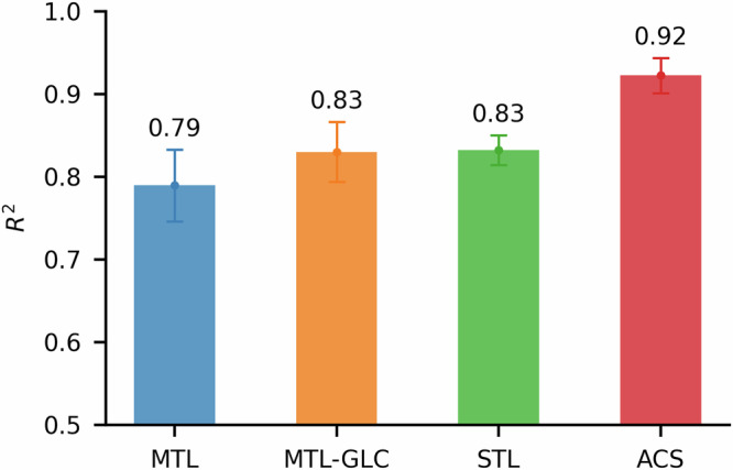
Average performance of MTL, MTL-GLC, STL, and ACS.

The advantage of ACS is especially pronounced in the ultra-low-data regime, where it achieves a 20.3% average performance gain over the other methods (Fig. 4, left). STL, which lacks inductive transfer, often fails on tasks with fewer than 60 samples. MTL and MTL-GLC do benefit from parameter sharing but still suffer from NT when large task imbalances occur. In contrast, ACS effectively mitigates NT, permitting beneficial inductive transfer even for tasks with minimal labeled data. As shown in Supplementary Notes 3, ACS maintains robust performance across all tasks, whereas the other methods show substantial variability in the ultra-low-data regime. Close inspection of MTL-GLC reveals that it can outperform STL for tasks with extremely scarce labels (owing to its inherent inductive transfer) but tends to underperform on tasks for which STL does not fail, leading to comparable overall performance. Conventional MTL shows the weakest performance overall, likely because it shares parameters without sufficient regularization against NT and lacks the higher task-specific capacity inherent to STL.

Fig. 4. Data regime-segmented performance comparison between the various training schemes over the SAF dataset.

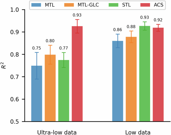
Performance of MTL, MTL-GLC, STL, and ACS over the ultra-low (left) and low (right) data regimes.

In the low-data regime (150 < n < 800), STL performance becomes comparable to that of ACS (Fig. 4, right), suggesting that tasks with larger datasets can fully leverage STL’s dedicated learning capacity. MTL and MTL-GLC also improve in this regime, as tasks with more labeled samples gain greater influence over network parameters. Nonetheless, ACS consistently provides robust performance across both data regimes, highlighting its effectiveness in scenarios with significant task imbalance and limited data availability.

Task-relatedness manifests in ACS backbones

In MTL, inductive transfer occurs when the training signals or learned representations from one task enhance the performance of another. Because ACS uses a shared backbone while allowing each task to maintain specialized parameters, tasks that are truly related produce backbones with similar latent representations. Inversely, limited task-relatedness is expected to reduce performance gains from ACS (See Supplementary Notes 5 for a detailed discussion). To investigate this effect, we calculated the cosine similarity between the final graph embeddings of each SAF dataset molecule across the task-specific backbones. For a given pair of task-specific latent vectors (u, v), the cosine similarity is defined as $\frac{\mathit{u}\cdot \mathit{v}}{∣∣\mathit{u}∣∣\mid \mid \mathit{v}\mid \mid }$. Higher similarity values indicate stronger alignment between task-specific backbone parameters. This alignment reflects convergent learning: although each backbone is optimized for a different property, related tasks discover overlapping representational structures in the molecular latent space. Because these embeddings are learned independently from a shared input, consistent alignment suggests the presence of common underlying molecular patterns or physical mechanisms. To account for any molecule-specific anomalies, we compute this metric separately for each molecule and then average the results across all molecules in the SAF dataset, yielding a single value for each pair of tasks. Figure 5 highlights the task pairs that rank in the top 10% for cosine similarity, corresponding to ≥ 0.96 similarity (see Supplementary Notes 4 for 15%, 20%, and 50% thresholds). Several task pairs display exceptionally high alignment, indicating that they capture shared underlying physical mechanisms or chemical features. These findings confirm that ACS can effectively harness inductive transfer by preserving meaningful commonalities among related tasks, while still allowing for task-specific specialization.

Fig. 5. Task similarity analysis.

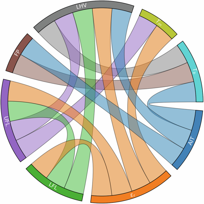
Chord diagram of the GNN backbones with the 10% highest cosine similarity between their latent space vectors, averaged over the entire dataset.

To illustrate these high-similarity relationships in more detail, consider autoignition temperature (AIT) and normal boiling point ($T_b$). This pair exhibits a striking correlation of 0.996, consistent with previous quantitative structure-property relationship (QSPR) models³². This strong correlation reflects how both properties hinge on how readily a compound transitions to the vapor phase before ignition. Given that $T_b$ is the temperature at which vapor pressure ($P_v$) equals atmospheric pressure, we find that their ACS backbones are highly correlated (~0.986). The lower and upper flammability limits (LFL and UFL) also exhibit a correlation in terms of backbone parameters, producing a cosine similarity of 0.988. It is unsurprising that the flash point (FP) correlates at 0.974 with $T_b$, given that both properties depend strongly on volatility as demonstrated by previous QSPR studies^33,34. In the same high-similarity tier, pairs such as UFL and melting point ($T_m$) (~0.971) or AIT and lower heating value (LHV) (~0.969) illustrate how shared structural factors—such as chain length, functional groups, and intermolecular interactions—underlie ignition and phase-transition behaviors³².

Furthermore, we find LHV aligning with vapor pressure ($P_v$) (~0.972), as well as viscosity ($\mu$) correlating at 0.991 with $T_b$. Both reflect how molecular weight and polarity simultaneously elevate boiling point, heat of combustion, and viscosity^35,36. Meanwhile, moderate similarities arise among properties such as cetane number (CN) and surface tension (ST) (~0.836), or liquid heat capacity ($C_p$) and $T_b$ (~0.802). Here, chain length and intermolecular forces still play a role, albeit in different physical systems (spray ignition behavior versus thermophysical measurements). Finally, correlations drop further when bridging distinct phases or conditions, for example, liquid thermal conductivity (κ) and $T_b$ (~0.531), or liquid density ($\rho$) and $T_m$ (~0.389). This reduction in correlation arises because the physics governing liquid-phase transport at moderate temperatures differ substantially from those governing boiling or solid-phase transitions.

One way to visualize correlations between latent space representations is through universal manifold approximation and projection (UMAP), a dimensionality reduction technique that preserves the local and global structure of high-dimensional data. Figure 6 displays UMAP projections for two of the aforementioned highly correlated task pairs, with colors indicating molecular families. While UMAP plots may differ in orientation due to the method’s invariance to rotation and reflection, the underlying structure remains consistent. For instance, the heart-shaped clustering in the AIT projection closely resembles that of $T_b$, albeit rotated by 180 degrees (Fig. 6a, b). A similar correspondence is observed for the flammability limits (LFL, UFL), where both projections show nearly identical clustering arrangements across chemical families (Fig. 6c, d).

Fig. 6. Task similarity analysis.

UMAP projections of two pairs of highly correlated tasks, with molecules colored by their chemical family. Related tasks exhibit similar clustering patterns in the latent space. The epoch values listed represent the epoch of last validation loss reduction. a AIT. b $T_b$. c LFL. d UFL.

These visual similarities are further supported by analyzing the placement of specific chemical families. In both LFL and UFL projections, n-Alcohols cluster tightly in the same region of the second quadrant, indicating that the two task-specific backbones project these molecules in a consistent manner. Likewise, the AIT and $T_b$ backbones position n-Alcohols along a prominent vertical pattern, which remains recognizable despite a 180-degree rotation between the two projections. When accounting for this rotational invariance, the embeddings of unsaturated aliphatic esters also align closely between AIT and $T_b$, occupying similar regions relative to other chemical families. These consistent, family-specific projections across related tasks suggest that task-specialized backbones tend to embed chemically similar molecules into structurally analogous regions of latent space—even in the absence of explicit chemical family supervision.

Moreover, the epoch of the last validation loss reduction supports the notion that similar tasks tend to receive positive parameter updates during consistent training intervals. Specifically, AIT and $T_b$ converged at epochs 341 and 333, corresponding to 47.0% and 46.0% of the total 725 training epochs, respectively. Likewise, LFL and UFL reached their final improvements at epochs 479 and 529—66.0% and 73.0% of training. These tightly grouped convergence points indicate that, despite differences in task label counts and complexity, related tasks tend to converge within similar portions of training, reflecting shared inductive learning dynamics.

Computational cost of training and inference

MTL can offer substantial computational gains whenever multiple downstream tasks share core representational requirements, thanks to parameter sharing in a unified model. This advantage often grows with both the number of tasks and model complexity. In our practical SAF property-prediction scenario, for example, MTL trained 11.5 times faster than the STL baseline while requiring only 6% of the trainable parameters, as shown in Table 2. These figures reflect our specific choice of model architecture, in which approximately 43% of the total parameters lie in the GNN backbone, and each prediction head only accounts for a small fraction of the parameters. Sharing this complex GNN backbone among tasks drastically reduces the overall training cost in MTL; however, a smaller backbone architecture would likely diminish this difference in speed relative to STL.

Table 2.

Trainable parameters and measured training time for ACS, MTL, MTL-GLC and STL for training using the SAF dataset

Training scheme	Training time (hours / fold)	GNN parameters	MLP parameters	Total parameters
ACS MTL MTL-GLC	1.85 1.57 1.82	$4.62\times {10}^6$	$6.13\times {10}^6$	$1.07\times {10}^7$
STL	18.04	$1.62\times {10}^8$	$6.13\times {10}^6$	$1.68\times {10}^8$

All timings were measured on an NVIDIA V100 32 GB GPU.

Despite more frequent checkpointing in ACS, we observed no significant increase in training time compared to MTL-GLC (as shown in Table 2). This result underscores the computational efficiency of ACS’s approach to mitigating negative transfer, even when running multiple training instances. The computational cost of checkpointing results in ~ 17% longer training time for ACS and MTL-GLC compared to MTL, highlighting the utility of low-overhead checkpointing techniques. Notably, molecular property prediction for material design applications typically requires simultaneous estimation of multiple performance indicators (e.g., stability and toxicity)^5,6,37, making approaches like ACS especially well-suited for real-world design problems. By leveraging shared representations, such multi-property prediction methods streamline chemical space exploration and accelerate the discovery of viable molecular candidates.

Discussion

Our findings demonstrate that ACS provides a robust, data-efficient strategy for overcoming negative transfer in multi-task molecular property prediction. By combining a shared GNN backbone with task-specific heads—and selectively preserving parameters when a task’s validation loss reaches a new minimum—ACS strikes an effective balance between leveraging shared representations and shielding individual tasks from harmful updates. Across multiple molecular benchmarks, ACS matched or exceeded the performance of leading supervised approaches, confirming the importance of neutralizing conflicting gradients. Importantly, ACS preserves the benefits of high-complexity backbones even in severely imbalanced datasets, preventing tasks with large data from overshadowing those with minimal labels.

The practical relevance of ACS is underscored by its application to SAF property prediction, where it enables effective inductive transfer across 15 different tasks. In this scenario, ACS substantially reduced the number of training samples needed for accurate modeling. Notably, reliable predictions were obtained with as few as 29 labeled points in the ultra-low-data regime—an outcome unattainable with STL or conventional MTL. By drastically lowering the data requirements for accurate property prediction, ACS has the potential to reduce the duration of experimental workflows from years to months in typical materials discovery pipelines, thereby accelerating the pace of discovery and reducing the innovation latency in data-driven materials design. These results also highlight how task imbalance interacts strongly with model complexity, intensifying the potential for negative transfer. ACS mitigates this by retaining a model checkpoint before its parameters are adversely altered by NT or noisy gradient descent updates.

Moving forward, future experiments will systematically explore how variations in data characteristics and degree of task-relatedness can either enhance model synergy or exacerbate negative transfer. While this study focused on data scarcity and task imbalance, future studies should investigate other NT drivers, including optimal learning rate mismatch and data distribution differences. We anticipate that these insights will further refine the conditions under which multi-task learning remains both practical and effective in data-scarce domains. Furthermore, addressing the computational cost of checkpointing can alleviate the current memory and latency overheads: sparse or low-rank difference snapshots, on-the-fly re-computation of rarely used layers, and asynchronous validation schedules are all promising avenues. These improvements should make ACS scalable to hundreds of tasks and suitable for deployment in resource-constrained platforms.

It remains unclear whether datasets composed of entirely disjoint task subsets—where no molecule is labeled for more than one task—permit any meaningful cross-task learning. Evaluating ACS under such conditions would clarify whether its checkpointing strategy provides advantages beyond what is achievable with standard STL baselines. Lastly, incorporating task prioritization or scheduling mechanisms could further enhance ACS’s ability to manage imbalance-driven disparities in parameter influence, allowing low-resource tasks to exert appropriate influence on shared representations. In parallel, future versions of ACS may benefit from initializing the shared backbone using meta-learned or pre-trained weights. Such hybrid approaches could accelerate convergence and improve generalization when labeled data is scarce, while still leveraging ACS’s strengths in handling task imbalance and sparse supervision.

Methods

Model architecture

Our framework comprises a shared GNN backbone and separate MLP heads—one head per prediction task. The GNN backbone consists of edge-conditioned convolutional layers³⁸, each followed by a non-linear activation. Edge-conditioned layers incorporate bond information into the node update step, enabling the model to learn both atomic and bond-level features simultaneously.

Downstream of the backbone, each task is associated with a dedicated six-layer MLP that uses a cascading neuron configuration (i.e., hidden-layer sizes decrease progressively with depth). These MLP heads allow for task-specific learning while leveraging the shared latent representation generated by the GNN backbone. An ablation study utilizing a common MLP (matching the total parameter count of the task-specific MLPs) for all targets shows that task-specific MLPs achieve 38.7% higher performance than the common MLP.

Molecular graph construction

We use the PyTorch Geometric library³⁹ to convert molecular SMILES strings into graph-based encodings. Each molecule is represented as a graph whose nodes correspond to atoms and whose edges represent chemical bonds. Node (atomic) features include atomic number, chirality, formal charge, hybridization, aromaticity, and ring membership, among others. Edge (bond) features capture attributes such as bond type and stereochemistry. Table 3 summarizes the complete set of features used for both nodes and edges.

Table 3.

List of atom and bond features used in molecular graphs

Atomic Feature	Description	Bond Feature	Bond Description
Atomic Number	Number of protons in the nucleus.	Bond Type	Single, double, triple, etc.
Chirality	Type of chirality (e.g., none, tetrahedral, etc.).	Bond Stereochemistry	Cis/trans or other configurations.
Number of Bonds	Number of bonds the atom forms with other atoms.	Conjugation	Whether the bond is conjugated (e.g., alternating single and double bonds in an aromatic ring).
Formal Charge	Charge based on the number of electrons gained or lost.
Number of Hydrogens	Number of hydrogen atoms bonded to the atom.
Number of Radical Electrons	Number of unpaired electrons in the atom.
Hybridization Type	Type of hybridization of the atom’s orbitals (e.g., sp, sp2, sp3).
Aromaticity	Whether the atom is part of an aromatic ring.
Ring Membership	Whether the atom is part of a ring structure.

Node features are stored in a feature matrix of size ($N\times d_{node}$), where $N$ is the number of atoms and $d_{node}$ is the dimensionality of node features. Similarly, edge features are stored in an edge feature matrix of size ($E\times d_{edge}$), where $E$ is the number of bonds. By passing these representations through the edge-conditioned convolutional layers, the model learns to aggregate information across nodes and edges in a task-agnostic latent space. Finally, each molecule’s latent representation is funneled into the task-specific MLP heads for final property prediction.

Adaptive checkpointing

Adaptive checkpointing continuously monitors the validation loss for each task and creates a checkpoint whenever a task’s validation loss decreases relative to its previous checkpoint. At these points, the current parameters of the shared backbone and the task-specific head are saved, ensuring that each task retains its best-known parameter state. By isolating these checkpoints, ACS mitigates negative transfer from other tasks in subsequent training steps. Table 4 presents pseudocode summarizing the training procedure.

Table 4.

Adaptive checkpointing training scheme

1. Randomly initiate model parameters

2. for training step $S_k$; 1:1:last_step do

a. Perform mini-batch training steps until the next validation step

b. for each task $T_i$; $i$=1,2,3… N do

i. Calculate per-task validation loss ${{loss}_{val}}_{S_k,T_i}$

1. if ${{loss}_{val}}_{S_k,T_i}>{{loss}_{val}}_{S_k-1,T_i}$ continue

2. else checkpoint backbone and ${head}_{T_i}$

3. Output: N task-specialized backbone and head pairs

At the end of the training, each task has an associated pair of backbone and head parameters corresponding to the best observed validation loss for that task. This strategy promotes effective inductive transfer while guarding against NT, ultimately enhancing performance across diverse and potentially imbalanced tasks.

Loss masking for missing values

We implemented a masking scheme (as shown in Fig. 7) within the loss function to maximize the use of training data. This approach selectively incorporates only valid data points, ignoring missing target values, while computing the error between predictions and targets. The final loss is normalized over the total number of target elements, ensuring robustness across varying dataset sizes. Unlike complete-case analysis, this method retains all available data without discarding samples, leading to more effective dataset utilization. Additionally, it mitigates the risk of poor generalizability associated with imputing missing values.

Fig. 7.

Loss masking process adopted for handling missing target values.

Uncertainty-informed loss function

For the SAF property prediction application, each training sample includes an associated uncertainty value ${\sigma }_i$, either sourced directly from experimental records or estimated based on the measurement procedure. To incorporate these uncertainties into model training, we scale the squared error term for each sample by $\alpha /\left(\alpha +{\sigma }_i\right)$, where $\alpha$ is a small-valued user-defined parameter. An $\alpha$ of 0.1 was found suitable for our SAF dataset. The resulting uncertainty-aware mean squared error $\left({MSE}_{UA}\right)$ for n samples is given by Eq. 2:

$${MSE}_{UA}=\frac{1}{n}{\sum }_{i-1}^n{\frac{\alpha }{\alpha +{\sigma }_i}\cdot \left(Y_i-{\widehat{Y}}_i\right)}^2$$ 2

This formulation penalizes the model less for errors on samples with high uncertainty, preventing noisy measurements from disproportionately influencing parameter updates. An ablation study revealed that incorporating uncertainty in this manner boosted the model’s 5-fold cross-validation performance by approximately 1.6%.

Datasets curation and pre-processing

Benchmark datasets

To illustrate the advantages of ACS and delineate its domain of applicability, we selected a subset of MoleculeNet benchmarks²¹ —datasets that feature multiple downstream tasks and are tractable for parametric evaluations. The three benchmark datasets which satisfy these requirements—ClinTox, SIDER, and Tox21—are described in the subsequent sections.

Each dataset was partitioned into training, validation, and test sets (8:1:1) using Murcko scaffolds²², following standard practice^{23–25,40,41}. This scaffold-based strategy ensures structural diversity across the splits, yielding a more robust test of model generalization.

To assess how effectively ACS mitigates negative transfer under varying conditions, we systematically adjusted task imbalance, as defined by Eq. (1), covering a broad range of imbalance scenarios. Concretely, we artificially introduced missing values into the CT_TOX column to achieve the desired level of imbalance, while retaining only a fraction of the overall samples to emulate a smaller dataset. By controlling this factor—ranging from heavily imbalanced, low-data scenarios to relatively balanced, data-rich conditions—we could pinpoint when ACS delivers the greatest benefit and when it remains competitive with conventional MTL and STL.

ClinTox

The ClinTox dataset consists of small molecules labeled according to their outcomes in clinical trials, specifically distinguishing compounds that were approved by the U.S. Food and Drug Administration (FDA) from those that failed due to toxicity issues. It comprises two binary classification tasks: FDA approval status and clinical trial failure due to toxicity. ClinTox presents a relatively small number of labeled molecules (1478) and is fully labeled without missing entries.

SIDER

The SIDER dataset contains marketed drugs annotated with adverse drug reaction information. In its MoleculeNet version, it is formulated as 27 independent binary classification tasks, each indicating whether a compound is associated with a specific side-effect category. The dataset includes 1427 molecules and is fully populated without missing labels.

Tox21

Tox21 is a benchmark dataset derived from the Tox21 initiative, providing chemical compounds evaluated across 12 biological assays related to nuclear receptor signaling and stress response pathways. Each task is a binary classification problem reflecting whether a compound is active or inactive in a given assay. The dataset includes 7,831 molecules, with an overall missing-label rate of approximately 17%.

SAF properties dataset

To validate the practical utility of ACS, we applied it to a real-world scenario involving the prediction of SAF properties. In particular, we curated a dataset of 1379 molecules commonly found in various SAF blends, compiling only experimentally measured or rigorously derived physical and chemical property values. Any records generated by predictive models were excluded to ensure data reliability. As part of a comprehensive screening, we set an upper uncertainty limit of 5% on experimental uncertainty and discarded any entries exceeding this threshold.

The set of SAF properties spans a wide range of physicochemical characteristics relevant to performance, operability, and drop-in compatibility with aviation systems. For example, the LHV strongly influences aircraft payload capacity and travel range, making it critical for flight efficiency. Similarly, the CN is an important certification requirement for assessing a fuel’s resistance to lean blow-out during engine operation⁴². A detailed description of the prediction tasks and property definitions within the SAF dataset is provided in the Supplementary Information. Due to the high rate of missing labels in the SAF dataset, the 8:1:1 split (train, validation, test) used for the benchmark datasets was not feasible. Instead, we employed a 5-fold CV approach, which provided more robust estimates of model performance while accommodating the inherent sparsity of the SAF data. The coefficient of determination, $R^2$, was used as a global performance metric to accommodate the variety in physical units across SAF properties.

Author contributions

B.A.E. and D.K. developed the methodology, wrote the code and analyzed the data. S.M.S. supervised the study. All authors contributed to writing and approved the final paper.

Peer review

Peer review information

Communications Chemistry thanks Mingyue Zheng and the other, anonymous, reviewers for their contribution to the peer review of this work.

Data availability

The training data used for all benchmark datasets analyzed in this study are publicly accessible through Zenodo: 10.5281/zenodo.15662353. This repository contains the datasets necessary to reproduce the results reported in this work. The raw data used to produce the figures in this paper are available in Supplementary Data 1.

Code availability

The full source code supporting this work is openly available on Zenodo 10.5281/zenodo.15662353 and the GitHub repository: https://github.com/BasemEr/acs. These repositories include all code scripts and implementation details required to reproduce the experiments and results presented in this study.

Competing interests

The authors declare no competing interests.

Supplementary information

The online version contains supplementary material available at 10.1038/s42004-025-01592-1.

References

- 1.Aleksić, S., Seeliger, D., & Brown, J. B. ADMET Predictability at Boehringer Ingelheim: State‐of‐the‐Art, and Do Bigger Datasets or Algorithms Make a Difference? Mol. Inform., 41, Feb. 10.1002/minf.202100113 (2022). [DOI] [PubMed]
- 2.Rittig, J. G., Ben Hicham, K., Schweidtmann, A. M., Dahmen, M. & Mitsos, A. Graph neural networks for temperature-dependent activity coefficient prediction of solutes in ionic liquids. Comput Chem. Eng.171, 108153 (2023). [Google Scholar]
- 3.Blanco-González, A. et al. The role of AI in drug discovery: challenges, opportunities, and strategies. Pharmaceuticals16, 891 (2023). [DOI] [PMC free article] [PubMed] [Google Scholar]
- 4.Aldeghi, M. & Coley, C. W. A graph representation of molecular ensembles for polymer property prediction. Chem. Sci.13, 10486–10498 (2022). [DOI] [PMC free article] [PubMed] [Google Scholar]
- 5.Sarathy, S. M. & Eraqi, B. A. Artificial intelligence for novel fuel design. Proc. Combust. Inst.40, 105630 (2024). [Google Scholar]
- 6.Allenspach, S., Hiss, J. A. & Schneider, G. Neural multi-task learning in drug design. Nat. Mach. Intell.6, 124–137 (2024). [Google Scholar]
- 7.Ruder, S. “An Overview of Multi-Task Learning in Deep Neural Networks,” arXiv preprint arXiv:1706.05098, (2017).
- 8.Caruana, R. Multitask learning. Mach. Learn28, 41–75 (1997). [Google Scholar]
- 9.Zhang, W., Deng, L., Zhang, L. & Wu, D. A survey on negative transfer. IEEE/CAA J. Autom. Sin.10, 305–329 (2022). [Google Scholar]
- 10.Yu, T. et al. “Gradient Surgery for Multi-Task Learning,” in Proc. 34th Annu. Conf. Neural Information Processing Systems (2020).
- 11.Wang, Z., Tsvetkov, Y., Firat, O., & Cao, Y., “Gradient Vaccine: Investigating and Improving Multi-task Optimization in Massively Multilingual Models,” in Proc. 9th Int. Conf. Learning Representations, Vienna, Austria, (2021).
- 12.Jiang, J. et al., “ForkMerge: Mitigating Negative Transfer in Auxiliary-Task Learning,” in Advances in neural information processing systems36, (2023).
- 13.Apicella, A., Isgrò, F., & Prevete, R., Don’t Push the Button! Exploring Data Leakage Risks in Machine Learning and Transfer Learning (2024).
- 14.Salazar, J. J., Garland, L., Ochoa, J. & Pyrcz, M. J. Fair train-test split in machine learning: Mitigating spatial autocorrelation for improved prediction accuracy. J. Pet. Sci. Eng.209, 109885 (2022). [Google Scholar]
- 15.Sheridan, R. P. Time-split cross-validation as a method for estimating the goodness of prospective prediction. J. Chem. Inf. Model53, 783–790 (2013). [DOI] [PubMed] [Google Scholar]
- 16.Wu, S., Zhang, H. R., & Ré, C. “Understanding and Improving Information Transfer in Multi-Task Learning,” in Proceedings of the International Conference on Learning Representations, (2020).
- 17.Lee, M. The geometry of feature space in deep learning models: a holistic perspective and comprehensive review. Mathematics11, 2375 (2023). [Google Scholar]
- 18.Yi, J., Lee, J., Kim, K. J., Hwang, S. J., & Yang, E., “Why Not to Use Zero Imputation? Correcting Sparsity Bias in Training Neural Networks,” in International Conference on Learning Representations (2020).
- 19.Little, R. J., Carpenter, J. R. & Lee, K. J. A comparison of three popular methods for handling missing data: complete-case analysis, inverse probability weighting, and multiple imputation. Socio Methods Res53, 1105–1135 (2024). [Google Scholar]
- 20.Gilmer, J., Schoenholz, S. S., Riley, P. F., Vinyals, O., & Dahl, G. E., “Neural message passing for quantum chemistry,” in International conference on machine learning, PMLR, 1263–1272. (2017).
- 21.Wu, Z. et al. MoleculeNet: a benchmark for molecular machine learning. Chem. Sci.9, 513–530 (2018). [DOI] [PMC free article] [PubMed] [Google Scholar]
- 22.Bemis, G. W. & Murcko, M. A. The properties of known drugs. 1. Molecular frameworks. J. Med. Chem.39, 2887–2893 (1996). [DOI] [PubMed] [Google Scholar]
- 23.Boulougouri, M., Vandergheynst, P. & Probst, D. Molecular set representation learning. Nat. Mach. Intell.6, 754–763 (2024). [Google Scholar]
- 24.Wang, Y., Wang, J., Cao, Z. & Barati Farimani, A. Molecular contrastive learning of representations via graph neural networks. Nat. Mach. Intell.4, 279–287 (2022). [Google Scholar]
- 25.Fang, Y. et al. Knowledge graph-enhanced molecular contrastive learning with functional prompt. Nat. Mach. Intell.5, 542–553 (2023). [Google Scholar]
- 26.Yang, K. et al. Analyzing learned molecular representations for property prediction. J. Chem. Inf. Model.59, 3370–3388 (2019). [DOI] [PMC free article] [PubMed] [Google Scholar]
- 27.Xu, Y., Ma, J., Liaw, A., Sheridan, R. P. & Svetnik, V. Demystifying multitask deep neural networks for quantitative structure–activity relationships. J. Chem. Inf. Model57, 2490–2504 (2017). [DOI] [PubMed] [Google Scholar]
- 28.Gayvert, K. M., Madhukar, N. S. & Elemento, O. A data-driven approach to predicting successes and failures of clinical trials. Cell Chem. Biol.23, 1294–1301 (2016). [DOI] [PMC free article] [PubMed] [Google Scholar]
- 29.Artemov, A. V. et al. Integrated deep learned transcriptomic and structure-based predictor of clinical trials outcomes. 10.1101/095653 (2016).
- 30.ASTM International, ASTM D7566, Standard specification for aviation turbine fuel containing synthesized hydrocarbons. 10.1520/D7566-22A (2022).
- 31.ASTM International, ASTM D4054-23, Standard practice for evaluation of new aviation turbine fuels and fuel additives. 10.1520/D4054-23 (2018).
- 32.Baskin, I. I. et al. Autoignition temperature: comprehensive data analysis and predictive models. SAR QSAR Environ. Res31, 597–613 (2020). [DOI] [PubMed] [Google Scholar]
- 33.Katritzky, A. R., Petrukhin, R., Jain, R. & Karelson, M. QSPR Analysis of Flash Points. J. Chem. Inf. Comput Sci.41, 1521–1530 (2001). [DOI] [PubMed] [Google Scholar]
- 34.Gharagheizi, F., Keshavarz, M. H. & Sattari, M. A simple accurate model for prediction of flash point temperature of pure compounds. J. Therm. Anal. Calorim.110, 1005–1012 (2012). [Google Scholar]
- 35.Mansouri, K., Grulke, C. M., Judson, R. S. & Williams, A. J. OPERA models for predicting physicochemical properties and environmental fate endpoints. J. Cheminform.10, 10 (2018). [DOI] [PMC free article] [PubMed] [Google Scholar]
- 36.Diaz, M. G. et al. Prediction of the heats of combustion for food-related organic compounds. A quantitative structure–property relationship (QSPR) study. J. Therm. Anal. Calorim.149, 11747–11759 (2024). [Google Scholar]
- 37.Siramshetty, V. B., Xu, X., & Shah, P. Artificial Intelligence in ADME Property Prediction 307–327. (2024). [DOI] [PubMed]
- 38.Simonovsky, M., & Komodakis, N. “Dynamic edge-conditioned filters in convolutional neural networks on graphs,” in Proceedings of the IEEE Conference on Computer Vision and Pattern Recognition, 3693–3702. (2017).
- 39.Fey, M. & Lenssen, J. E., “Fast graph representation learning with PyTorch Geometric,” arXiv preprint arXiv:1903.02428, (2019).
- 40.Fang, X. et al. Geometry-enhanced molecular representation learning for property prediction. Nat. Mach. Intell.4, 127–134 (2022). [Google Scholar]
- 41.Ross, J. et al. Large-scale chemical language representations capture molecular structure and properties. Nat. Mach. Intell.4, 1256–1264 (2022). [Google Scholar]
- 42.Zheng, L. et al. Experimental study on the impact of alternative jet fuel properties and derived cetane number on lean blowout limit. Aeronaut. J.126, 1997–2016 (2022). [Google Scholar]
- 43.Kipf, T. N., & Welling, M. “Semi-Supervised Classification with Graph Convolutional Networks,” in Proceedings of the 5th International Conference on Learning Representations, (2016).
- 44.Xu, K., Hu, W., Leskovec, J. & Jegelka, S.“How Powerful are Graph Neural Networks?” in Proc. 7th International Conference on Learning Representations (2018).
- 45.Schütt, K. T., Sauceda, H. E., Kindermans, P.-J., Tkatchenko, A. & Müller, K.-R. “SchNet – A deep learning architecture for molecules and materials,” J. Chem. Phys.148., 10.1063/1.5019779. (2018). [DOI] [PubMed]
Associated Data
This section collects any data citations, data availability statements, or supplementary materials included in this article.
Supplementary Materials
Description of Additional Supplementary Files
Data Availability Statement