Analyzing the impact of export tax rebates and energy conservation on sustainable industrial growth in China

Abstract

When China implemented the exports tax rebate policy through administrative framework in 1985, industrial energy consumption increased by more than five times. The purpose of this study is to examine the relationship between industrial energy demand (IED), exports tax rebate, exports, and the value of industrial output in the presence of other variables such as GDP, taking into account the effects of carbon dioxide (CO₂) and foreign direct investment (FDI). The present study adopted the Autoregressive-Distributed Lag (ARDL) model and Granger Casuality analysis of the VECM to examine the short run and long relationship among different variables. The empirical evidence supported the long-term cointegration of these pasrameters and demonstrated a positive impact on industrial energy consumption. Foreign direct investment reduces the need for industrial power. The conservation hypothesis between export tax credits and industrial energy use was also verified by the Granger Causality analysis of the VECM. Furthermore, export tax credits have a secondary impact on energy use in manufacturing. This research might lead to more effective legal or adminsitarive regulations and policy measures to curb China’s rising energy use in the industrial sector.

Introduction

According to the world energy outlook projects (WEO2013), energy consumption will continue to increase the global carbon emissions from 31.3Gt in 2011 to 37.2Gt in 2035 unless and until tremendous efforts are made to control energy consumption and carbon emission^1–3. Since, China approved trade openness in 1978, industrial and economic growth has been accelerated, requiring more energy to fulfill industrial energy demand and making China the world’s biggest energy consumer^4,5. China utilized 3.27 billion tonnes of oil equivalents in 2018, accounting for 23.6% of world energy⁶. Whereas a significant percentage of China’s aggregate energy consumption goes to its industrial sector, in 2022, it consumed 3.490 billion tons of SCE, with a 64.5% share out of 5.415 billion tons of total energy consumption⁷. Figure 1 shows a time series analysis of China’s overall energy usage and industrial energy consumption between 1985 and 2022. Furthermore, burning fossil fuels releases dangerous gases called greenhouse gases⁸. China has become the world’s largest source of carbon dioxide emissions, making up 27.3% of all carbon dioxide emissions⁹. But, to stop pollution and emissions from hurting the environment, the State Council of China has made plans to reduce the use of non-renewable power in key industrial sectors. Additionally, China has introduced a national action plan for reducing energy consumption and emission reduction to GDP as of 2030 by more than 65% compared to 2005¹⁰. Hence, to fulfill these ambitious objectives of reduction in energy consumption, it is indispensable for all sectors to find effective options to curb environmental pollution.

Fig. 1.

China’s overall energy use as well as energy use in the industrial sector. Source : Author’s constructed.

China introduced the export tax rebate policy in 1985 to make the products competitive in the international market by keeping the product prices low¹¹. Many studies have shown that the export tax rebate has a positive effect on exports and the production of goods for export^12,13, With a continuous increase in China’s export tax rebate from 17.95 billion RMB in 1985 to 15,154 billion RMB in 2022, the exports of goods were also substantially augmented from 808.9 hundred million RMB in 1985 to 24,200 hundred million RMB in the year 2022⁷. This rapid increase in exports of goods labeled China as the largest international trade partner globally¹⁴. Although, the global energy agency declared that in 2004, China’s 34% carbon emission was caused by the production of goods to meet international consumers’ demand^14,15. But the question arises, “Does exports and export tax rebate affect China’s industrial energy consumption?” This research aims to address this topic regarding China’s industrial power usage, exports, and export tax rebate (ETR).

As threats to the environment worsened, many local and international researchers became very interested in reducing energy use and carbon emissions. So, different studies examine the relation among things like energy use, exports, economic growth, foreign direct investment (FDI), urbanization, population growth, carbon emissions, trade, etc., to figure out how the environment is getting worse and what kind of regulations and policies can be made to curb the situation^16,17, But, there are two common limitations in these studies; first, all the studies of this kind considered aggregate energy consumption to relate to other variables but, remarkably, industrial energy consumption was not considered the largest energy-consuming sector in China. Second, to the author’s best knowledge, most research studies were conducted to evaluate the association between trade or trade openness and energy consumption. But there was no research found that looked into the link between the trade tax rebate regulation and the amount of energy needed by industries. Thus, studying the new relationship between industrial energy demand and export tax rebates in China is indispensable to avoid ambiguity.

The four acceptances of this study are a significant addition to the literature. (1) China’s industrial sector uses most of the country’s energy, so this paper focuses on that sector instead of the country’s total energy consumption. This differs from other studies, which have examined the country’s total energy consumption. (2) The study in hand research uses export tax rebates rather than real commerce to explore the link between industrial energy usage and exports¹⁸. (3) The present study applys ARDL bound test, the Granger causality test, and any other relevant tests to evaluate whether or not there is a link and, if so, what its future course will be. (4) This study’s potential benefits for reducing energy consumption and mitigating adverse environmental effects are enhanced using current data.

The remaining parts of the article are organized as follows: The literature review is dissected and discussed in more detail in the second half of the study. The third portion is going to be devoted to the presentation of the methodological framework. The research results are dissected and evaluated in great depth in the fourth section of the report. The conclusion discussion is supposed to take place in the fifth part, immediately followed by the reference section at the very end.

Literature review

Alarming global warming has drawn attention to environmental protection from all stakeholders around the globe, including academia and policymakers. Therefore, plenty of research has been conducted to reduce energy consumption to mitigate environmental pressure in the recent past. The abundant literature used time series or panel data to minimize environmental pollution using different variables. The present study will divide the existing literature into three categories to help the readers to understand the literature on energy and the environment; first, scholarly work on energy usage and economic development in the context of certain other factors. The second is the environmental Kuznets curve (EKC) hypothesis or halo and heaven theory, which looks at the relationship between pollution and economic growth. Third, studies mainly focus on energy efficiency improvements by different policy tools. A brief discussion about the first two categories in the existing literature is discussed in the below sections. The energy efficiency improvement-related literature is not addressed in this study due to the nature of the present study.

Energy use, economic growth, foreign direct investment (FDI), and carbon emission

Energy became the burning research issue as it is the driving factor for development and is considered a significant cause of environmental pollution¹⁹. examined the impact of economic growth, energy prices, digitalization, and climate policy uncertainty and the findings of the key macroeconomic, technological, and political factors on ESG performance in the U.S. within a comprehensive sustainability framework to mitigate climate change^20,21. Conservation, Growth, Feedback, as well as Neutrality Assumptions) put the existing literature on energy consumption into four groups and explained what each one meant.

Conservation hypothesis: An increase in per capita income causes a corresponding increase in per capita energy use; this is another causation between economic growth and energy consumption. There is a wealth of evidence supporting the conservation hypothesis, such as the study by²² that looked at the feasibility of absolute decoupling between Ghana and the United Kingdom by 2030. Rising GDP combined with falling energy demand is the decoupling effect. According to the results of the research, it is very unlikely that the two nations in the sample would ever be able to achieve a complete decoupling of energy from their financial development. Furthermore, a 2% increase in energy consumption is needed to satisfy Ghana’s annual 5% economic growth rate. Growth in Pakistan’s energy consumption and the gross domestic product was studied²³. Using yearly data from 1971 to 2014, the author used a non-linear autoregressive lag model. The study revealed a non-linear relationship between Pakistan’s energy use and GDP growth. Coal use in Indonesia was studied to determine the results of economic growth, industrialization, urbanization, and freer trade²⁴. The investigation results demonstrated the presence of cointegration between the variables, as mentioned earlier.

Additionally, the results indicated that urbanization, trade openness, and economic growth influenced the increase in coal consumption between 1970 and 2015. Azam et al. (2016)²⁵ Greek energy consumption was examined using yearly data between 1975 and 2013, looking at the impact of socio-economic factors. According to the VECM model, important drivers of energy consumption in Greece are FDI, population growth, commerce, and infrastructure development. Furthermore, the report suggested looking into alternate ways to meet the country’s expanding energy need to boost Greece’s economic growth²⁶. The ARDL model was utilized to determine how FDI, GDP, and trade openness affect the UAE’s energy needs. The results of the study showed that these factors are linked together. In addition, the data showed that economic development and clean energy increase energy demand, but FDI, CO₂ emissions, and trade openness decrease UEA energy consumption. Numerous writers performed numerous relevant research in diverse places, including:^27–29, .

Growth Hypothesis: According to the growth theory, if energy consumption increases, the economy will expand. The causal link between rising energy use and expanding economies. Several perspectives on the growth hypothesis have been considered. Between 2004 and 2017, Huang and Huang (2019)³⁰ analyzed data on China’s energy consumption, GDP growth, FDI, exports, imports, and urbanization. According to the ARDL model, rising energy consumption results from increasing urbanization, rising imports and exports, and growing FDI. China’s fast economic expansion, on the other hand, is in large part due to the country’s high energy consumption. Between 1995 and 2014, Hao et al. (2018)³¹ analyzed the connection between energy consumption, financial development, and economic growth in 29 Chinese provinces using panel data. From what we can tell, Granger’s energy use helps 29 different Chinese provinces prosper economically. However, Granger argues that expanding the financial sector does not boost the economy. The ARDL model Akalpler & Hove, (2019) and time series data have been used to analyze the growth of the Indian economic system between 1971 and 2014¹⁸. The results showed that many factors contributed to the economy’s short-term growth, including energy consumption, gross fixed capital, carbon emissions, and imports. Exports have a crucial role in India’s long-term economic development, whereas Mahalingam and Orman, (2018) investigated panel data from various U.S. states to establish if economic expansion drives energy demand or whether energy demand drives economic growth³². How these elements interact depends on geography, according to the study. Mostly in southern U.S., economic growth drives energy consumption, whereas energy consumption drives economic growth in the Rocky States. To balance the state’s economic growth and energy usage, a federal energy strategy was created. Several studies advocate expansion:^33–35.

Feedback Hypothesis: Economic growth must exceed energy consumption to achieve hypnosis. Shahbaz et al. (2019) utilized an Autoregressive Distributed Lag Model to analyze the factors that influence the U.S. energy demand function (ARDL). Long-term data indicates that export diversification and education have a negative impact on energy use. In contrast, individuals consume less energy as the economy expands. When the price of oil increases, people use less energy, but when they utilize natural resources, they consume more energy. A Granger Causality analysis also points to a two-way connection connecting energy consumption to economic growth in the USA³⁶. Tiba and Frikha (2018)³⁷ used simultaneous equations to analyze panel data from 24 high- and middle-income countries between 1990 and 2011 to establish the connection involving energy use, GDP, and trade openness. Results from a sample of medium to high and intermediate countries corroborated the hypothesis that higher energy use is associated with lower income and that more trade openness is correlated with higher wages. However, in nations with a high per capita income, the relationship between trade openness as well as energy use is one-sided. Middle-income countries used more energy and were more trade-friendly at the same time. Kilinc and Rehman (2024)³⁸ examined how urbanization, energy pricing, and per capita economic development influenced the energy consumption of 186 nations between 1986 and 2005. Panel cointegration and panel causality tests were used to investigate the relationship between the variables. The sample was separated into three groups based on the individuals’ income levels (i.e., lower middle, upper middle, and high income countries). Long-term correlations were found between the variables, and a causality analysis showed that economic expansion and energy use are linked in both directions. The numbers also showed that urbanization increases energy use in countries with lower and high incomes but not those with upper middle incomes. Wang et al. (2014)³⁹ used panel data from 30 Chinese provinces between 1995 and 2011 to examine the relationship across urbanization, energy use, and carbon emissions. The findings of the panel data model revealed that carbon emissions vary by location over the sample period and that CO₂ emissions decrease from the east coast to the midwest to the west coast. In addition, the data demonstrated that energy consumption, carbon emissions, and urbanization had a reciprocal, long-term link. In addition, scenario modeling revealed that China’s carbon emissions would continue to rise from 2012 to 2020. The majority of energy consumption studies demonstrate the feedback effect, and there is a great deal of relevant literature^40–42.

Neutrality Hypothesis: Studies by^42–44 suggest that power consumption will have little to no influence on economic development, lending credence to the neutrality theory.

Environmental pollutants, GDP, trade, FDI, halo and Heaven hypothesis, EKZ

Other literature discusses the EKC theory, pollution halo, and heaven hypothesis. Pollutants (Carbon emission, Wastewater, NO, SO₂, etc.) are usually the dependent variable. Other variables, including foreign investment, economic growth, energy consumption, etc., test the EKZ, pollution halo, and heaven hypothesis. Chen and Taylor, (2020)⁴⁵ analyzed the EKZ in Singapore by using chromium as a surrogate for the destruction of the environment. Research showed a U-shaped negative association with economic growth on Cr in Singapore, validating EKZ. Data showed that Singapore’s post-industrialization caused the pollution heaven effect. Using the STIRPAT model and China provincial panel data, Xu et al. (2019)⁴⁶ investigated the impact of financial development, FDI, R&D, and exports on air pollutants. Exports reduced air pollution, according to the research.

On the other hand, foreign direct investment decreased pollution in all three places, which backs up the idea of a “pollution heaven.” Air pollution went down in part because of research and development. Compared to each other, industrialization and population growth caused air pollution to worsen in all three places. Also, the analysis showed that as the economy grew, air pollution went up and followed an inverted N-shaped trend. This disproved the EZK theory for the region under investigation. Using panel data from 11 newly industrialized states between 1977 and 2013, Destek and Sarkodie, (2019)⁴⁷ analyzed the EKZ by examining the connection with growth in the economy, financial sector development, power consumption, and ecological footprints. Using the augmented estimation prediction model, researchers could see that economic growth and ecological footprints had an inverted U-shaped connection. Studies on EKZ, pollution halos, and the concept of heaven are expanding^48–50.

Exports, exports tax rebate, and industrial energy demand

A lot of research shows that importing and exporting goods positively affects how much energy is used. For example, Cole (2006)⁵¹ used the fixed-effect technique to study a group of 32 developed and developing countries to determine if there was a link between trade liberalization and energy use. In the sample, there were both developed and developing countries. The research shows that opening up trade positively affects the total energy used in a certain amount of time. Ghani, (2012) did a study to find out how the liberalization of trade would affect how developing countries use their energy resources. Based on the results of this research, it seems that trade liberalization does not immediately affect the amount of energy spent; but, at a certain level of economic development, there is a rise in the amount of energy used⁵². While Zheng et al., (2011) used panel data from 20 Chinese sub-industries to examine how increased exports affected energy intensity, they did not account for the effect of export tax refunds⁵³. This is because the study did not take into account the data from 1999 to 2007. This is because the data from the research conducted between 1999 and 2007 were never considered at any stage of the analytic procedure. In addition, to keep the study’s breadth within reasonable bounds, the inquiry was limited to only twenty distinct types of industrial sub-sectors.

On the other hand, there was nothing about export tax rebates on energy use in industry in the existing literature. Most of the research that has been done up to this point has been about how export tax refunds affect business. For instance, Zhang (2019) investigated the relationship between export tax refunds and company productivity in China by using the GMM model¹². Only a few other studies have examined the link between the export tax rebate and trade or exports. Some of these studies are;^11,54. On the other hand, a few authors looked at how the export tax rebate affects the environment by using the CGE model. For example, Eisenbarth (2017) looked into it and found that export taxes and the export tax rebate in China are affected by environmental pollution⁵⁵. Song et al. (2015) found that export tax breaks in China lead to pollution of the environment⁵⁶. Using the CGE model, a different study (Fan et al., 2015) found a link between China’s trade tax rebate as well as CO₂ emissions¹³. Although there is a wealth of literature on energy and the environment, the link between industrial energy use, export tax refunds, and exports does not seem to have gotten much attention in the existing literature. This is even though there is a lot of printed material on energy and the environment. As a result, to fill a gap in the previously published research, the current study has been designed to investigate the influence tax breaks for exports and exports have on the amount of energy China’s industrial sector consumes.

Research methods and data descriptions

In order to study the impact of export tax rebates on energy conservation in China, the present study used different variables such as China total energy consumption, export tax rebates, GDP, FDI. The data for energy consumption for aquired from China’s annual energy yearbook⁵⁷. The statistical yearbook of China was used to find out how much an export tax rebate was in billion RMB and how much the gross industrial output was in 100 million RMB⁵⁷. On the other hand, we got information from the world development indicator about GDP, FDI, CO₂, and exports⁵⁸.

Model specifications

In order to assess the effect of export tax refunds on energy consumption in industry, the authors of the current research developed an econometric model, denoted by Eq. 1.

1

All the variables were changed into natural log representation using the equation as shown by Eq. 2, which significantly reduced heteroscedasticity.

2

Whereas , and are the long-term elasticity forecasts of manufacturing energy consumption (E) for trade tax rebate (ETR), gross industrial output (Y), Gdp growth (GDP) at existing USD, foreign direct investment (FDI), export (EXP), and carbon emission (CO₂), respectively. At the same time, ln is the natural log of all the variables, and t is the period from 1985 to 2022.

Procedure of estimation

Unit root test

When the two different time series are added together, the result can be stationary. If it stays the same, the series is cointegrated and there is a long-term relationship between them⁵⁹. Riti et al. (2017) say that the ARDL method doesn’t need a pre-test of the non-stationary characteristics of the data, but it is important to look into the series data properties of the variables⁶⁰. So, the current study used Augmented Dicky Fuller to check if the time series data were stationary, taking into account the benefit of independence from different lag lengths in individual ADF regressions, as suggested by⁶¹. The ADF unit root test is mathematically described in Eq. (3).

3

Whereas; Represents the time series variable for testing the stationarity and Shows the error term. Equation (3) pits the alternative hypothesis that > 0 against the null hypothesis that = 0. The time series y t is deemed stationary if and only if it is negative and statistically significant. The Bayesian information criteria evaluated the ideal lag durations using the ADF unit root test.

ARDL bound testing approach for cointegration test

According to Uddin et al. (2013), typical synchronization approaches do not provide accurate results when there are structural issues with the data⁶². Therefore, Auto Regressive League (ARDL) bound testing, was developed by⁶³. Pesaran et al. (2001) determine how well the variables are cointegrated⁶⁴. The ARDL method has already been shown to work with small samples⁶⁵. It could also solve the problems of bias and autocorrelation⁶⁴. Also, the method usually gives long-term models and a fair estimate of unreliable T statistics, even when endogeneity is a factor (Harris and Sollis, 2003). For our study, this is how we came up with the experimental form of the ARDL equation:

4

5

6

7

8

9

10

The VECM Granger casualty test

According to Granger (1969), using a brief Granger Causality trial for such Regression Model (VECM) may determine whether the variables are related in the same order⁶⁶. We chose the short-term and long-term directions that would be beneficial since the whole variable remains constant at the initial difference I (1). The findings have more policy consequences when the beneficial connection leads in the appropriate direction⁶⁷.The following VECM specification showed the probabilistic model of this study in different ways:

11

Diagnostic tests

Various diagnostic tests, including the Lagrange Multiplication (L.M.) testing for autocorrelation, the Ramsay RESET testing for research model, the reliability analysis for heteroscedasticity, and models stabilization graphical layout tests, were conducted (e.g., CUSUM and CUSUM).

Empirical results and discussions

Pearson correlation

A list of variables and their connections to one another in Table 1 may be used for correlation analysis. Table 1 shows that all of the factors we looked at had a significant correlation with energy use, with some having a coefficient of up to 90%. Certainly, export tax rebates, exports, FDI, GDP, and industrial output positively affected energy demand (E), with 97.3%, 98.8%, 92.6%, 99.1%, and 97.8%, respectively. However, at the same time, the Pearson correlation of energy demand and Co₂ was found to be highly positive and significant. It has been veiled that economic indicators are detrimental to Industrial energy demand in China. Our results are similar to those⁶⁸, demonstrating a strong correlation across export, energy consumption, and carbon emission in China.

Table 1.

Pearson correlation.

	Ln E	Ln ETR	Ln CO2	Ln EXP	Ln FDI	Ln GD	Ln Y
Ln E	1
Ln ETR	0.973**	1
Ln CO2	0.892**	-0.931**	1
Ln EXP	0.988**	0.984**	-0.927**	1
Ln FDI	0.926**	0.958**	-0.951**	0.958**	1
Ln GDP	0.991**	0.953**	-0.900**	0.984**	0.919**	1
Ln Y	0.978**	0.983**	-0.960**	0.992**	0.974**	0.978**	1

**. Correlation is significant at the 0.01 level (2-tailed).

Author’s tabulation.

Data diagnostic test

The various diagnostic procedures were used to evaluate the ARDL model’s performance and the data’s dependability. An examination is made of the Breusch-Pagan-Godfrey model, a tool for determining whether or not variance exists. The value of Chi-Square is shown to be 0.7899 in Table 2, which does not constitute a significant number. This indicates that the model’s residuals do not exhibit any signs of heteroscedasticity. In addition, the heteroscedasticity test was successful under ARCH and white tests, demonstrating that the values of 2-statics (0.9405 and 0.2431) are insignificant for the estimates. This indicates that the dataset does not have any issues related to heteroscedasticity. These findings provide credence to our study since they validate our assumptions, such as the fact that the model does not include any outliers or absent variables⁶⁹, demonstrating that our data are accurate.

Table 2.

Heteroscedasticity test.

Particular	Prob. Chi-Square	Obs*R-squared	F-statistic	Prob. F
Breusch-Pagan-Godfrey	0.7899*	9.613573	0.50525	0.8951
Harvey	0.4535*	13.94929	0.93115	0.5506
Glejser	0.6552*	11.39014	0.65576	0.7818
ARCH	0.9405*	0.005578	0.005194	0.9431
White	0.2431*	29.51099	2.845561	0.0977

* Chi-Square probability value is insignificant at the 0.05 level of significance.

Author’s tabulation.

Descriptive statistics and normality test

The facts about the Chinese economy are shown in Table 3. The table illustrates the data’s characteristics, including the average, maximum, minimum, standard error, kurtosis, skewness, and Jerqa-Bera standardized tests. According to the skewness and kurtosis values shown in Table 3, the questioned dataset did not include any skewness or other anomalies. According to the research, an increase in industrial output of 11.52% results in an average rise in carbon emissions of around 52.10 million tonnes. The export tax rebate scheme boosted industrial production and increased energy consumption by 12.08%, according to¹³. These results are comparable to those stated in that research. In addition, the normalcy problem is assured by a Jerqa Bera analysis, which is also shown in Table 3; most of the variable values are insignificant, indicating that results are drawn from a standard normal distribution.

Table 3.

Descriptive statistics and normality test.

Particulars	Ln CO2	Ln ETR	Ln Y	Ln GDP	Ln E	Ln FDI	Ln EXP
Mean	0.521039	7.0359	11.5204	7.1044	12.0862	24.4026	26.4302
Median	0.392040	6.9706	11.5658	6.9128	11.9046	24.5436	26.2931
Maximum	1.2451	9.4624	13.5199	9.0017	12.9854	26.3963	28.5323
Minimum	0.0512	2.8875	9.1159	5.5286	11.2474	21.2294	23.9736
Std. dev	0.3362	1.8432	1.3658	1.1794	0.5538	1.6475	1.5485
Skewness	0.6368	-0.3461	-0.2020	0.2813	0.2367	-0.6425	-0.0616
Kurtosis	2.2958	2.1362	1.87227	1.7254	1.6896	2.1907	1.6112
Jarque-Bera	2.8244	1.6338	1.9134	2.5882	2.5884	3.0750	2.5919
Probability	0.2436**	0.4417**	0.3841**	0.2741**	0.2741**	0.2149**	0.2736**

** The probability value is not significant at the 0.05 threshold of significance.

Author’s tabulation.

The augmented Dicky fuller unit root test

The first thing that you need to do is investigate the relationship between the variables at a level and after the first difference. To determine whether or not there was an issue with the time series data being stationary, we used the ADF unit root test. The first assumption of this test first established the concept of a unit root issue. The second assumption said that data doesn’t have a unit core issue. It is assumed that this test has an intercept term or a trend seen from the intercept. The AIC criterion carefully and independently chose the number of lags. The results of the ADF unit root test are shown in Table 4. They show that the variables Y, GDPpc, E, and EXP are not stationary at I(0), even though their mean and standard deviation are (1). It means that the link between these variables will last for a long time, which is why cointegration analysis is needed⁷⁰. Also, the data showed that other important factors, like CO₂, ETR, and FDI, are still the same. So, the tests for stationary statistics show that neither of the variables chosen is stable at the second level I (2).

Table 4.

ADF unit root testing.

Particulars	Level		First Difference		Results
	t- statistics	Probability value	t- statistics	Probability value
Ln CO2	--3.0854**	0.0032	-4.0962*	0.0035	I(0)c
Ln ETR	-3.1242**	0.0350	-4.5117*	0.0013	I(0)a
Ln Y	-1.8695	0.6432	-3.8840**	0.0271	I(1)b
Ln GDP	-2.7250	0.2343	-3.0779**	0.0391	I(1)a
Ln E	-2.1870	0.4792	-2.9872**	0.0476	I(1)a
Ln FDI	-3.7028**	0.0105	-3.3864**	0.0196	I(0)a
Ln EXP	-1.2318	0.6477	-4.5114*	0.0012	I(1)a

*, **, *** stationary at 1%, 5% and 10% significant levels respectively.

^a Results with intercept only.

^b Results intercept and trend both are included.

^c Represents results with none.

Author’s formulations & tabulation.

Testing bounds technique with ARDL

The F-statistic test is used to see if factors are connected in the long term or not. If the value of f - statistic is greater than the critical value of the topmost relationship, the regress and regressors may be connected in the long term. The critical value represents that the results are not conclusive if they fall anywhere between the upper and lower limits (Wong and Hook, 2018). Table 5 shows that the bound testing method found that the F statistics value (F = 12,757) is higher than both the lower bound I (0) and the maximum bound I (1). At a significance level of 5%, the fact that the F-statistic value in Table 5 is outside the upper and lower limits shows that the variables being looked at with the ARDL constraint have kept their long-term integration. On the other side, Wang et al. (2021) demonstrated that there is no correlation between the quantity of a nation’s exports and the overall amount of carbon emissions the country produces over a significant time⁷¹. Their findings were published in the journal Environmental Research Letters. This is because new technical advancements increase the overall quality of production while simultaneously decreasing the amount of energy required for production as a whole.

Table 5.

ARDL bound test and F-statistic.

F-statistics	12.75748***
Critical value %	1%	5%	10%
Lower bound I(0)	3.15	2.45	2.12
Upper bound I(1)	4.43	3.61	3.23

*** Significant at the 1% level.

Author’s tabulation.

ARDL long run co-integration

Various findings presented in Table 6 have been obtained from the ARDL long-run test. Energy consumption is significantly related to the five regressors (export tax rebate, gross industrial production, foreign investment, trade, and Carbon pollution (CO₂). However, conversely, in long-term estimations, GDP per capita has an insignificant association with industrial energy demand in China. Concisely, China’s increasing level of carbon emission, GDPpc, and gross industrial output are positively and significantly interconnected with industrial energy demand (E). While the GDPpc has demonstrated a weak correlation in the data we have examined. Yet, at the 5% significance threshold, an export tax refund is favorably associated with industrial energy use. An increase or decrease of 1% in Chinese exports and Foreign direct investment in the long term suggested an increase or decrease of 0.0191 and 0.22% in China’s industrial energy consumption, respectively. Findings from the studies cited by Fan et al. (2015) and Chen et al., (2006) suggest that inferences are examined similarly, which is helpful for the results obtained^13,72.

Table 6.

ARDL long run co-integration.

Particulars	Coefficient	Standard. Error	t-Statistic	Probability
Ln ETR	0.157491	0.042636	-3.693815	0.0209**
Ln CO2	0.294633	0.100669	2.926742	0.0430**
Ln EXP	-0.019106	0.031849	-0.599909	0.5809***
Ln FDI	-0.220228	0.045283	-4.863413	0.0083*
Ln GDP	0.158530	0.097181	1.631288	0.1782
Ln Y	0.836018	0.177648	4.706043	0.0093*
Constant	7.939331	0.735125	10.799971	0.0004*

*, **, *** stationary at 1%, 5% & 10% significant level respectively.

Authors’ formulations & tabulation.

Export tax rebate is an essential trade policy. It is refunded money of product taxes, VAT, corporate taxes, and a special type of consumption taxes paid by manufacturers or retailers during the domestic manufacturing and distribution phase. Consequently, the positive interrelationship between export tax rebate policy and industrial output immediately changed the Chinese pattern of trade to boost local exports. China emerged on the global stage as an export-oriented nation after the first phase of this program was implemented and completed. Not only did this approach increase exports, but it also assisted Chinese manufacturers in keeping their products at the forefront of global competition.

Why does the Chinese government need to take these drastic measures? In line with⁷³, the Vietnam government adopted a similar strategy, “Doi Moi” to improve its economic health. The initiative’s primary goal was to free up the economy, which a centralized planning authority had previously controlled, and make it more responsive to market forces. So, the government gave exporters and investors many chances to invest in key areas of development. This helped stabilize the country’s economic growth and raise the income of each household per person. So, our econometric analysis has shown that there is a positive link between export tax rebate, export earnings, industrial output expansion, foreign investment, and economic growth. A 1% change in tax breaks for exports shows that industrial energy demand and exports have changed significantly.

In the modern era of Chinese transformation, domestic exports have become a key element of china’s economic stability. Therefore, China produced manufactured products at a massive level to meet the international market’s demand and fulfill their own nationals’ needs. The Chinese economy is heavily reliant on industrial energy demand. It is needed to make goods and provide services, which is crucial for China’s industrial growth. According to Nnaji et al. (2013), if the country used its energy resources well enough to meet demand, industrial development would be higher, which would encourage exports and help the economy grow⁷⁴. Table 6 shows that exports and industrial energy demand have had a long-term, positive relationship. It has been shown that a rise in industrial products within the limits of energy use increases exports and helps the economy grow.

Furthermore, Table 6 certifies that export tax rebates enhance exports and industrial output growth, consequently increasing industrial energy demand and CO₂ emissions in China. Due to the huge amount of trade China does with the rest of the world, these assumptions are based on industrial goods that require a lot of energy. So, this is a growing movement in trade and industry that makes carbon emissions more intense quickly^75,76.

ARDL short-run cointegrations

The Akaike Criteria lags selection method is the basis for the ARDL bound testing protocol for cointegration. However apart from it, the ARDL uses the right slowdowns for all regression coefficients in a way that allows it to predict the future (5, 1, 2, 2, 2, 2, and 2). The proper criteria for choosing the lag are predicated on the AIC. We used a “5” for the predictor variables energy demand, a “1” for the most critical variable, which is the export tax rebate, and a “2” for the other regressors. Table 7 shows the short-term link between China’s export tax rebate policy and the positive parameters for industrial output and industrial energy demand. Inferences showed that trade rebate reforms throughout China directly increase industrial output growth in the near term but may also hurt the development of the economy and exports in a long time.

Table 7.

ARDL short term co-integration.

Variable	Coefficient	Std. Error	t-Statistic	Prob.
D(LN E(-1))	1.081105	0.297516	3.633776	0.0221*
D(LN E(-2))	0.423701	0.341324	1.241345	0.2823
D(LN E(-3))	3.131791	0.491391	6.373315	0.0031*
D(LN E(-4))	1.173650	0.239710	4.896127	0.0081*
D(LN CO2)	0.827593	0.134035	6.174435	0.0035*
D(LN EXP)	-0.259237	0.096738	-2.679783	0.0552***
D(LN EXP(-1))	-0.153714	0.047567	-3.231520	0.0319**
D(LN FDI)	0.000008	0.036519	0.000212	0.9998
D(LN FDI(-1))	0.226117	0.039656	5.701985	0.0047*
D(LN GDP)	-0.695868	0.217100	-3.205287	0.0327**
D(LN GDP(-1))	-1.023861	0.167144	-6.125610	0.0036*
D(LN Y)	0.712899	0.327296	2.178146	0.0949***
D(LN Y(-1))	2.102181	0.309418	6.793994	0.0025*
D(LN ETR)	0.049577	0.035237	1.406956	0.2322
D(LN ETR(-1))	0.276107	0.053525	5.158497	0.0067*
CointEq(-1)	-1.919039	0.296429	-6.473865	0.0029*

*, **, *** stationary at 1%, 5% & 10% significant level respectively.

Authors’ formulations & tabulation.

Lag length ARDL(5, 1, 2, 2, 2, 2, 2).

Model selection method: Akaike info criterion (AIC).

R-squared	0.999914	Mean dependent var	12.21926
Adjusted R-squared	0.999444	S.D. dependent var	0.496705
S.E. of regression	0.011710	Akaike info criterion	-6.262556
Sum squared resid	0.000549	Schwarz criterion	-5.158695
Log likelihood	107.5445	Hannan-Quinn criter.	-5.934320
F-statistic	2126.100	Durbin-Watson stat	3.384339
Prob(F-statistic)	0.000000

Given the time required for policies to have their most beneficial impacts, these findings indicate that this industrial progress will not be able to compete with the global market in the near future. Growth in industrial production and increased energy use both lead to increasing carbon emissions, which are immediately harmful to the environment and will have lasting effects. Therefore, legislators and experts must consider the present when making policy choices that will reduce Emissions in the state. The ECT term was attracted by short-term ARDL, with a Coint Eq (-1) correlation coefficient of -1.9190, which is unfavorable but significant at the 1% level. The above findings demonstrated that the dependent and independent variables are connected over the long term. It’s also worth noting that the adjusted R-squared value is 0. (0.999444). The model is generally well-fitting, as shown by Durbin-Watson and F-statistic values, indicating that the significance threshold should be more than 5%. Since this is the case, we may conclude that the model is accurate. Retrieval results showed a D.W. value of 3.38 and an F-statistic of 2126. When evaluating the impact of several factors on Shina’s industrial energy consumption, a significance level of 1*** implies that the model is flawed.

The VECM Granger causality test

Granger causality analysis, which measures the direction of the correlations between two variables, was used to test the stability of estimates. Econometric analysis, using the Granger causality approach, is shown in Table 8. Estimates of industrial energy consumption in light of the export tax refund have been calculated, and these conclusions are consistent with the preliminary findings from the ARDL-bound testing strategy. China’s environmental quality and the rate of carbon dioxide emissions are impacted by factors like export tax rebate revisions, industrial production, energy consumption, and exports. In contrast, under Granger causality test, foreign direct investment and export rebate tax reforms have no direct linkages with CO₂ emissions. Every significant causality is assumed to operate in both directions so that changes in export tax rebates and the resulting energy demands of the industry may be seen as a cause of variation in other variables. As a result, it is established and confirmed that short-term changes in reforms, production, and energy consumption are significantly degrading the environment and fostering unease in the atmosphere and among living creatures.

Table 8.

The VECM granger causality test.

Null hypothesis		Observations	F-statistics	Probability
LN CO2 does not Granger Cause LNE		29	1.66275	0.2040
LN E does not Granger Cause LNCO2			2.35502	0.0996*
LN EXP does not Granger Cause LNE		26	3.49777	0.0277**
LN E does not Granger Cause LN EXP			2.21444	0.1082
LN GDP does not Granger Cause LNE		31	19.2614	0.0001***
LN E does not Granger Cause LN GDP			0.13499	0.7161
LN E does not Granger Cause LN FDI		31	0.01167	0.9148
LN FDI does not Granger Cause LNE			0.01273	0.9110
LN Y does not Granger Cause LNE		27	2.52398	0.0723*
LN E does not Granger Cause LN Y			1.20433	0.3513
LN ETR does not Granger Cause LNE		31	4.20274	0.0498**
LN E does not Granger Cause LN ETR			0.92859	0.3435
LN EXP does not Granger Cause LN CO2		30	4.73406	0.0181**
LN CO2 does not Granger Cause LN EXP			3.14988	0.0603
LN FDI does not Granger Cause LN CO2		31	1.86025	0.1835
LN CO2 does not Granger Cause LN FDI			0.11905	0.7326
LN GDP does not Granger Cause LN CO2		29	3.06878	0.0491**
LN CO2 does not Granger Cause LN GDP			0.86515	0.4739
LN Y does not Granger Cause LN CO2		29	3.89771	0.0225**
LN CO2 does not Granger Cause L.N. Y			0.01478	0.9975
LN ETR does not Granger Cause LN CO2		31	1.13606	0.2956
LN CO2 does not Granger Cause LN ETR			0.33023	0.5701
LN FDI does not Granger Cause LNE		31	2.03551	0.1647
LN EXP does not Granger Cause LN FDI			0.00351	0.9532
LN GDP does not Granger Cause LN EXP		29	3.14869	0.0454**
LN EXP does not Granger Cause LN GDP			3.64883	0.0283**
LN Y does not Granger Cause LN EXP		31	0.40350	0.5304
LN EXP does not Granger Cause LN Y			0.60253	0.4441
LN ETR does not Granger Cause LN EXP		31	4.34145	0.0464**
LN EXP does not Granger Cause LN ETR			8.54904	0.0068***
LN GDP does not Granger Cause LN FDI		30	0.04184	0.9591
LN FDI does not Granger Cause LN GDP			3.88996	0.0338**
LN Y does not Granger Cause LN FDI		31	0.03348	0.8561
LN FDI does not Granger Cause LN Y			5.45664	0.0269**
LN ETR does not Granger Cause LN FDI		31	2.68502	0.1125
LN FDI does not Granger Cause LN ETR			0.38011	0.5425
LN Y does not Granger Cause LN GDP		30	12.4737	0.0002***
LN GDP does not Granger Cause LN Y			6.95944	0.0040***
LN ETR does not Granger Cause LN GDP		30	6.67518	0.0048***
LN GDP does not Granger Cause LN ETR			0.49839	0.6134
LN ETR does not Granger Cause LN Y		31	8.70195	0.0064***
LN Y does not Granger Cause LN ETR			2.99156	0.0947

*, **, *** stationary at 1%, 5% & 10% significant level respectively.

Authors’ formulations & tabulation.

Graphical presentation of the VECM Granger causality test

The findings of the VECM Granger Causality test are summarized in Fig. 2, which also explains whether the link among the variables is unidirectional or bidirectional. The findings also indicate a unidirectional association between exports tax rebate and industrial output and a unidirectional association between industrial output and industrial energy demand. However, the results also indicate a bidirectional relationship between exports and export tax rebates. In addition, export tax rebates had a direct and unidirectional relationship with the amount of energy that industrial facilities required. Furthermore, other factors such as foreign direct investment (FDI), gross domestic product (GDP), and exports are essential predictors of industrial energy consumption.

Fig. 2.

The VECM Granger causality test.Author’s construction.

Impulse response test

The impulse response function is used to show a clearer picture of the model’s dynamic structure. The outcomes of the impulse response are specified in the graph. 1, which shows that at an initial level, the response function for energy demand, when to give a shock to export tax rebate reforms, appears positive in the earliest fourth span of time, and afterward bearing a slightly declining trend. In addition, the trend continues until period 9, when the numbers become positive. A single shock in energy demand provides a cause to alter other regressors until 4–10 periods dynamically; nevertheless, following this recovering the fluctuations mentioned above after the 10th period. Findings are the following Bhatt, (2013) found that industrial production concerning export tax refund is a major variable. In the long run, a rise in exports will lead to an increase in foreign direct investment (FDI)⁷³.

Graph 1.

Impulse response test. Source : Author’s constructed.

The CUSUM test and squared-CUSUM test

The stability of the coefficients in graphs 2 and 3 was evaluated using the CUSUM square test and the Cumulative Sum of Recursive Residuals test⁶⁴. The simultaneous graphical display supports the conclusion drawn from the ARDL model. The square CUSUM and the process CUSUM both work to guarantee that the blue line on both graphs is located within the red dots. In addition, the presentation sheds light on the fact that these factors are suitable for use with the dependent variable to make predictions. As stated by⁷⁷, the Chinese government should continue to work to improve industrial growth with the help of an export tax rebate policy and improve the social and environmental structure.

Graph 2.

CUSUM test. Source : Author’s constructed

Graph 3.

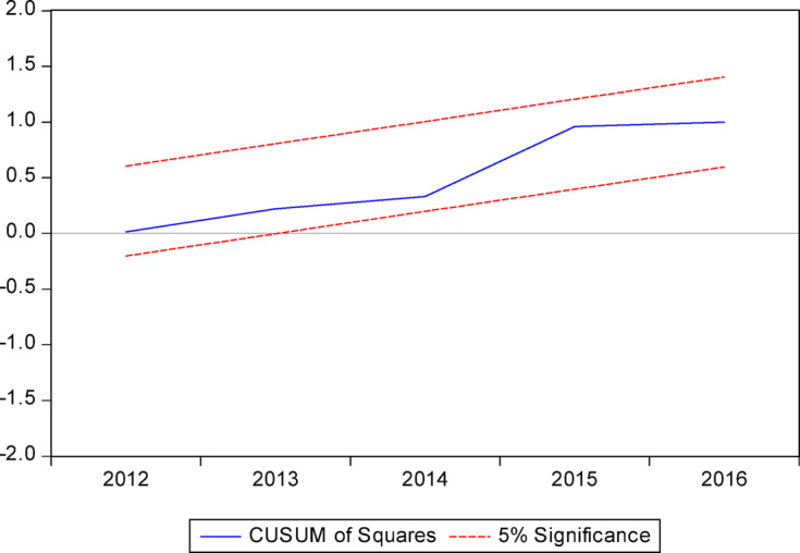
CUSUM square test. Source : Author’s graphical representation.

Discussion

The findings of the present study are inline with the existing literature such as⁷⁸ where the author found that there is a negative relationship between renewable energy consumption and CO₂. In another study⁷⁹, explored the role of economic, social, governance factors, climate policy uncertainty and carbon emissions. Using ARDL model, the author reveal that while economic factors increase CO₂ emission. Based on these results, Energy consumption driven by global economic growth and industrial production based mainly on fossil fuels increases CO2 emission. These findings are also in line with the present study as current study explained that key macroeconomic indicators such as GDP growth are increasing carbon emissions in China. At the same time, non renewable energy consumption also exerting a high pressure on carbon emission. The results are very obvision that China is a developing country and China’s economy mainly based on exports sector. Thus to meet the high international demand for export good and demostic use for different products, the industrial sector of China is accelerate its production. There to meet the demand for industrial production, the massive amount of energy is required which maninly comes from coal consumption in China that is largest sources for carbon emissions^5,80. Seconldy, China is the developing country, following the EKC theory, China does not have reached the peak, which means at this stage the carbon emission will be increasing with the increase in economic growth. Thus, the findings of the present study are aligned with existing literature and the economic theories. Moreover, based on the findings of these studies has suggest numarious polices such as, the export tax rebate should given to the industries with high energy efficieny and low carbon emissions. Moreover, the modernization of the industrial sector should be focused to counter the environmental pollution and to achieve the China’s dual carbon goals.

Conclusion and policy implications

Taking into account the findings and discussions above, it can be concluded that export tax rebates stimulated the industrial energy demand, which ultimately led to an increase in carbon emissions, despite being an important legal policy instrument to encourage industrial output growth and exports. Therefore, the Chinese government has established regulations to decrease energy consumption and carbon emissions to address the rising environmental threats worldwide. One essential policy tool to reduce China’s rising industrial energy consumption and carbon emissions is a revision of its exports tax rebate program, which will help the country achieve its lofty targets.

The first distinguishing feature of the present research is that it is the first to examine the effect of export tax refunds on China’s industrial energy consumption. The results of the ARDL model revealed that a tax credit for exporting industrial goods had a lasting effect on energy use. Additionally, the export tax refund boosted industrial production, increasing China’s industrial energy consumption. According to the numbers, firms cranked up their energy use in response to a surge in exports prompted partly by tax rebates. This was shown by exports going up after the refunds were given out. China’s industrial energy use is also affected positively by other factors, such as its FDI inflows and economic output. In short, we can say that the export tax rebate is an important policy tool that directly affects how much energy China’s industrial sector needs. As a result, China’s program for lowering carbon emissions and satisfying its energy requirements requires paying significant consideration to export tax refunds.

The current research results provide authorities in China’s industrial sector with legal and policy recommendations on how better to analyze the country’s export tax refund program. The present analysis concludes that fewer export rebates, or none, should be given on industrial outputs and exports from industries that cause a lot of pollution to cut down on pollution. Ultimately, this action would help reduce pollution. The Chinese government could provide refunds to the manufacturing sector that relies heavily on renewable energy sources by reevaluating its export tax rebate program. Moreover, the government should introduce incentives in the form of rebates to the industrial sector with high investment in research and development on energy efficiency improvements and emission reductions. The government should link the export tax rebates to the none renewable energy demand, research and development expenditure, and emission reduction targets. To further strengthen policy effectiveness, targeted strategies could include a classification mechanism that segments industries by their carbon intensity and energy efficiency. For instance, high-emission sectors should face stricter eligibility criteria for export rebates, while low-carbon industries could receive enhanced fiscal incentives. Moreover, rebate eligibility could be made conditional on firms disclosing their annual energy audits, sustainability reports, and demonstrated progress toward emission targets. These actions would ensure that tax rebates align more closely with national environmental and sustainability goals.

While the current research offered a novel energy and emission reduction policy design concept—namely, a tax refund for exports—a further investigation into this area is needed. As a result, studies are planned to examine the connection between export tax credits and R&D and renewable energy to gauge these policies’ effect on carbon dioxide emissions. As a bonus, the research may be organized to examine how energy-intensive firms in China benefit from export tax credits.

Author contributions

Miqdad Mehdi: Corresponding Author, Funding Provider, Writer and Conceptulization Bingqiang Li: SupervisorZulqarnain Mushtaq: Writer, Editor, Analysis, Data Availability.

Data availability

Data will be available on request. For data please contact Dr. Zulqarnain Mushtaq on zulqarnainmushtaq@yahoo.com.

Declarations

Competing interests

The authors declare no competing interests.

References

- 1.Işık, C., Yan, J. & Ongan, S. Energy intensity, supply chain digitization, technological progress bias in china’s industrial sectors. Energy Econ.145, 108442 (2025). [Google Scholar]
- 2.IEA, Global Energy Review: CO2 Emissions in 2020. (2021).
- 3.Kilinc-Ata, N. & Dolmatov, I. The Russian federation’s renewable energy development determinants: evidence from empirical research. Int. J. Energy Sect. Manage.17 (4), 779–800 (2023). [Google Scholar]
- 4.Wei, W. et al. Evaluating the coal rebound effect in energy intensive industries of China. Energy 118247. (2020).
- 5.Mushtaq, Z., Wei, W. & Liu, J. Unleashing China’s coal conservation potentials by analyzing efficiency of energy intensive industries: A Logarithm Mean Divisia Index (LMDI) model 0958305X241238328 (Energy & Environment, 2024).
- 6.BP. Statistical Review of world energy 2022. (2023).
- 7.Statistical-Yearbook Statistical Yearbook of China. State department of China: Beijing (2023).
- 8.Chen, W. & Xu, R. Clean coal technology development in China. Energy Policy. 38 (5), 2123–2130 (2010). [Google Scholar]
- 9.Zhang, Y. J., Peng, H. R. & Su, B. Energy rebound effect in china’s industry: an aggregate and disaggregate analysis. Energy Econ.61, 199–208 (2017). [Google Scholar]
- 10.NDRC Action plan for carbon dioxide peaking before 2030 (NDRC, Editor., 2021).
- 11.Chao, C. C., Chou, W. L. & Eden, S. Export duty rebates and export performance: theory and china’s experience. J. Comp. Econ.29 (2), 314–326 (2001). [Google Scholar]
- 12.Zhang, D. Can export tax rebate alleviate financial constraint to increase firm productivity? Evidence from China. Int. Rev. Econ. Finance. 64, 529–540 (2019). [Google Scholar]
- 13.Fan, J. L. et al. Will export rebate policy be effective for CO2 emissions reduction in china?? A CEEPA-based analysis. J. Clean. Prod.103, 120–129 (2015). [Google Scholar]
- 14.Chen, Y., Wang, Z. & Zhong, Z. CO2 emissions, economic growth, renewable and non-renewable energy production and foreign trade in China. Renew. Energy. 131, 208–216 (2019). [Google Scholar]
- 15.Outlook, A. E. Energy information administration. Dept. Energy. 92010 (9), 1–15 (2010). [Google Scholar]
- 16.Zhu, H. et al. The effects of FDI, economic growth and energy consumption on carbon emissions in ASEAN-5: evidence from panel quantile regression. Econ. Model.58, 237–248 (2016). [Google Scholar]
- 17.Zhang, Y. J. The impact of financial development on carbon emissions: an empirical analysis in China. Energy Policy. 39 (4), 2197–2203 (2011). [Google Scholar]
- 18.Akalpler, E. & Hove, S. Carbon emissions, energy use, real GDP per capita and trade matrix in the Indian economy-an ARDL approach. Energy168, 1081–1093 (2019). [Google Scholar]
- 19.Işık, C. et al. The nexus of economic growth, energy prices, climate policy uncertainty (CPU), and digitalization on ESG performance in the USA. Clim. Serv.38, 100572 (2025). [Google Scholar]
- 20.Tuna, G. & Tuna, V. E. The asymmetric causal relationship between renewable and NON-RENEWABLE energy consumption and economic growth in the ASEAN-5 countries. Resour. Policy. 62, 114–124 (2019). [Google Scholar]
- 21.Menegaki, A. N. & Tugcu, C. T. Two versions of the index of sustainable economic welfare (ISEW) in the energy-growth nexus for selected Asian countries. Sustainable Prod. Consum.14, 21–35 (2018). [Google Scholar]
- 22.Heun, M. K. & Brockway, P. E. Meeting 2030 primary energy and economic growth goals: mission impossible? Appl. Energy. 251, 112697 (2019). [Google Scholar]
- 23.Baz, K. et al. Energy consumption and economic growth nexus: new evidence from Pakistan using asymmetric analysis. Energy189, 116254 (2019). [Google Scholar]
- 24.Kurniawan, R. & Managi, S. Coal consumption, urbanization, and trade openness linkage in Indonesia. Energy Policy. 121, 576–583 (2018). [Google Scholar]
- 25.Azam, M. et al. Socio-economic determinants of energy consumption: an empirical survey for Greece. Renew. Sustain. Energy Rev.57, 1556–1567 (2016). [Google Scholar]
- 26.Sbia, R., Shahbaz, M. & Hamdi, H. A contribution of foreign direct investment, clean energy, trade openness, carbon emissions and economic growth to energy demand in UAE. Econ. Model.36, 191–197 (2014). [Google Scholar]
- 27.Kilinc-Ata, N., Camkaya, S. & Topal, S. What role do foreign direct investment and technology play in shaping the impact on environmental sustainability in newly industrialized countries (NIC)? New evidence from wavelet quantile regression. Sustainability17 (11), 4966 (2025). [Google Scholar]
- 28.Kilinc-Ata, N. Investigation of the impact of environmental degradation on the transition to clean energy: new evidence from Sultanate of Oman. Energies18 (4), 839 (2025). [Google Scholar]
- 29.Chiou-Wei, S. Z., Chen, C. F. & Zhu, Z. Economic growth and energy consumption revisited—evidence from linear and nonlinear Granger causality. Energy Econ.30 (6), 3063–3076 (2008). [Google Scholar]
- 30.Huang, Z. & Huang, L. Individual new energy consumption and economic growth in China. North. Am. J. Econ. Finance. 54, 101010 (2020). [Google Scholar]
- 31.Hao, Y., Wang, L. O. & Lee, C. C. Financial development, energy consumption and china’s economic growth: new evidence from provincial panel data. Int. Rev. Econ. Finance. 69, 1132–1151 (2020). [Google Scholar]
- 32.Mahalingam, B. & Orman, W. H. GDP and energy consumption: A panel analysis of the US. Appl. Energy. 213, 208–218 (2018). [Google Scholar]
- 33.Shakeel, M. & Iqbal, M. M. Energy consumption and GDP with the role of trade in South Asia. In: 2014 International conference on energy systems and policies (ICESP). IEEE. (2014).
- 34.Furuoka, F. Natural gas consumption and economic development in China and japan: an empirical examination of the Asian context. Renew. Sustain. Energy Rev.56, 100–115 (2016). [Google Scholar]
- 35.Ziaei, S. M. Effects of financial development indicators on energy consumption and CO2 emission of european, East Asian and Oceania countries. Renew. Sustain. Energy Rev.42, 752–759 (2015). [Google Scholar]
- 36.Shahbaz, M., Gozgor, G. & Hammoudeh, S. Human capital and export diversification as new determinants of energy demand in the united States. Energy Econ.78, 335–349 (2019). [Google Scholar]
- 37.Tiba, S. & Frikha, M. Income, trade openness and energy interactions: evidence from simultaneous equation modeling. Energy147, 799–811 (2018). [Google Scholar]
- 38.Kilinc-Ata, N. & Rahman, M. P. Digitalization and Financial Development Contribution To the Green Energy Transition In Malaysia: Findings from the BARDL Approach. In Natural Resources Forum (Wiley Online Library, 2024).
- 39.Wang, S. et al. Urbanisation, energy consumption, and carbon dioxide emissions in china: A panel data analysis of china’s provinces. Appl. Energy. 136, 738–749 (2014). [Google Scholar]
- 40.Zafar, M. W. et al. From nonrenewable to renewable energy and its impact on economic growth: the role of research & development expenditures in Asia-Pacific economic Cooperation countries. J. Clean. Prod.212, 1166–1178 (2019). [Google Scholar]
- 41.Ben-Salha, O., Dachraoui, H. & Sebri, M. Natural resource rents and economic growth in the top resource-abundant countries: a PMG Estimation. Resour. Policy. 74, 101229 (2021). [Google Scholar]
- 42.Yildirim, E., Aslan, A. & Ozturk, I. Energy consumption and GDP in ASEAN countries: Bootstrap-corrected panel and time series causality tests. Singap. Economic Rev.59 (02), 1450010 (2014). [Google Scholar]
- 43.Zeshan, M. & Ahmed, V. Energy, environment and growth nexus in South Asia. Environ. Dev. Sustain.15, 1465–1475 (2013). [Google Scholar]
- 44.Narayan, P. K. & Prasad, A. Electricity consumption–real GDP causality nexus: evidence from a bootstrapped causality test for 30 OECD countries. Energy Policy. 36 (2), 910–918 (2008). [Google Scholar]
- 45.Chen, Q. & Taylor, D. Economic development and pollution emissions in singapore: evidence in support of the environmental Kuznets curve hypothesis and its implications for regional sustainability. J. Clean. Prod.243, 118637 (2020). [Google Scholar]
- 46.Xu, S. C. et al. Regional differences in nonlinear impacts of economic growth, export and FDI on air pollutants in China based on provincial panel data. J. Clean. Prod.228, 455–466 (2019). [Google Scholar]
- 47.Destek, M. A. & Sarkodie, S. A. Investigation of environmental Kuznets curve for ecological footprint: the role of energy and financial development. Sci. Total Environ.650, 2483–2489 (2019). [DOI] [PubMed] [Google Scholar]
- 48.Ali, W., Abdullah, A. & Azam, M. Re-visiting the environmental Kuznets curve hypothesis for malaysia: fresh evidence from ARDL bounds testing approach. Renew. Sustain. Energy Rev.77, 990–1000 (2017). [Google Scholar]
- 49.Wang, H., Dong, C. & Liu, Y. Beijing direct investment to its neighbors: A pollution Haven or pollution halo effect? J. Clean. Prod.239, 118062 (2019). [Google Scholar]
- 50.Zhang, Y. & Zhang, S. The impacts of GDP, trade structure, exchange rate and FDI inflows on china’s carbon emissions. Energy Policy. 120, 347–353 (2018). [Google Scholar]
- 51.Cole, M. A. Does trade liberalization increase National energy use? Econ. Lett.92 (1), 108–112 (2006). [Google Scholar]
- 52.Ghani, G. M. Does trade liberalization effect energy consumption? Energy Policy. 43, 285–290 (2012). [Google Scholar]
- 53.Zheng, Y., Qi, J. & Chen, X. The effect of increasing exports on industrial energy intensity in China. Energy Policy. 39 (5), 2688–2698 (2011). [Google Scholar]
- 54.Chandra, P. & Long, C. VAT rebates and export performance in china: Firm-level evidence. J. Public. Econ.102, 13–22 (2013). [Google Scholar]
- 55.Eisenbarth, S. Is Chinese trade policy motivated by environmental concerns? J. Environ. Econ. Manag.82, 74–103 (2017). [Google Scholar]
- 56.Song, P., Mao, X. & Corsetti, G. Adjusting export tax rebates to reduce the environmental impacts of trade: lessons from China. J. Environ. Manage.161, 408–416 (2015). [DOI] [PubMed] [Google Scholar]
- 57.Energy-Yearbook China Energy Statistical Yearbook, in National Bureau of Statistics (China Statistics, 2023).
- 58.Worldbank World Development Indicators, in the World Bank 2018 (World Bank, 2023).
- 59.Engle, R. F. & Granger, C. W. Co-integration and error correction: representation, estimation, and testing. Econometrica: J. Econometric Soc., 251–276. (1987).
- 60.Riti, J. S. et al. Decoupling CO2 emission and economic growth in china: is there consistency in Estimation results in analyzing environmental Kuznets curve? J. Clean. Prod.166, 1448–1461 (2017). [Google Scholar]
- 61.Bilgili, F., Koçak, E. & Bulut, Ü. The dynamic impact of renewable energy consumption on CO2 emissions: a revisited environmental Kuznets curve approach. Renew. Sustain. Energy Rev.54, 838–845 (2016). [Google Scholar]
- 62.Uddin, G. S., Sjö, B. & Shahbaz, M. The causal nexus between financial development and economic growth in Kenya. Econ. Model.35, 701–707 (2013). [Google Scholar]
- 63.Pesaran, M. H. The role of economic theory in modelling the long run. Econ. J.107 (440), 178–191 (1997). [Google Scholar]
- 64.Pesaran, M. H., Shin, Y. & Smith, R. J. Bounds testing approaches to the analysis of level relationships. J. Appl. Econom.16 (3), 289–326 (2001). [Google Scholar]
- 65.Işık, C. et al. Exploring the commitment to sustainable development goals (SDGs)–the renewable energy and tourism demand nexus. Tour. Econ., 13548166251320691. (2025).
- 66.Granger, C. W. Investigating causal relations by econometric models and cross-spectral methods. Econo. J. Econo. Soc. 424–438. (1969).
- 67.Shahbaz, M., Khan, S. & Tahir, M. I. The dynamic links between energy consumption, economic growth, financial development and trade in china: fresh evidence from multivariate framework analysis. Energy Econ.40, 8–21 (2013). [Google Scholar]
- 68.Zhang, Y. J., Bian, X. J. & Tan, W. The linkages of sectoral carbon dioxide emission caused by household consumption in china: evidence from the hypothetical extraction method. Empir. Econ.54 (4), 1743–1775 (2018). [Google Scholar]
- 69.Bölük, G. & Mert, M. The renewable energy, growth and environmental Kuznets curve in turkey: an ARDL approach. Renew. Sustain. Energy Rev.52, 587–595 (2015). [Google Scholar]
- 70.Zhang, Y. J., Bian, X. J. & Tan, W. The linkages of sectoral carbon dioxide emission caused by household consumption in china: evidence from the hypothetical extraction method. Empir. Econ.54, 1743–1775 (2018). [Google Scholar]
- 71.Wang, Z. et al. Does export product quality and renewable energy induce carbon dioxide emissions: evidence from leading complex and renewable energy economies. Renew. Energy. 171, 360–370 (2021). [Google Scholar]
- 72.Chen, C. H., Mai, C. C. & Yu, H. C. The effect of export tax rebates on export performance: theory and evidence from China. China Econ. Rev.17 (2), 226–235 (2006). [Google Scholar]
- 73.Bhatt, P. Causal relationship between exports, FDI and income: the case of Vietnam. Appl. Econometrics Int. Dev.13 (1), 161–176 (2013). [Google Scholar]
- 74.Nnaji, C., Chukwu, J. & Uzoma, C. An econometric study of CO2 emissions, energy consumption, foreign trade and economic growth in Nigeria. In: Conference proceedings of the 5th Annual NAEE/IAEE International Conference organized by Nigerian Association for Energy Economics, held at Abuja, Nigeria. (2013).
- 75.Işık, C., Sirakaya-Turk, E. & Ongan, S. Testing the efficacy of the economic policy uncertainty index on tourism demand in USMCA: theory and evidence. Tour. Econ.26 (8), 1344–1357 (2020). [Google Scholar]
- 76.Işık, C. et al. Renewable energy, climate policy uncertainty, industrial production, domestic exports/re-exports, and CO2 emissions in the USA: a SVAR approach. Gondwana Res.127, 156–164 (2024). [Google Scholar]
- 77.Bento, J. P. C. & Moutinho, V. CO2 emissions, non-renewable and renewable electricity production, economic growth, and international trade in Italy. Renew. Sustain. Energy Rev.55, 142–155 (2016). [Google Scholar]
- 78.Işık, C. et al. Exploring how economic growth, renewable energy, internet usage, and mineral rents influence CO2 emissions: A panel quantile regression analysis for 27 OECD countries. Resour. Policy. 92, 105025 (2024). [Google Scholar]
- 79.Işık, C., Ongan, S. & Islam, H. Global environmental sustainability: the role of economic, social, governance (ECON-SG) factors, climate policy uncertainty (EPU) and carbon emissions. Air Qual. Atmos. Health. 18 (3), 851–866 (2025). [Google Scholar]
- 80.Wei, W. et al. Evaluating the coal rebound effect in energy intensive industries of China. Energy207, 118247 (2020). [Google Scholar]
Associated Data
This section collects any data citations, data availability statements, or supplementary materials included in this article.
Data Availability Statement