How many named species are valid?

Abstract

Estimates of biodiversity in both living and fossil groups depend on raw counts of currently recognized named species, but many of these names eventually will prove to be synonyms or otherwise invalid. This difficult bias can be resolved with a simple “flux ratio” equation that compares historical rates of invalidation and revalidation. Flux ratio analysis of a taxonomic data set of unrivalled completeness for 4,861 North American fossil mammal species shows that 24–31% of currently accepted names eventually will prove invalid, so diversity estimates are inflated by 32–44%. The estimate is conservative compared with one obtained by using an older, more basic method. Although the degree of inflation varies through both historical and evolutionary time, it has a minor impact on previously published background origination and extinction rates. Several lines of evidence suggest that the same bias probably affects more poorly studied, hyperdiverse living groups such as fungi and insects. If so, then current estimates of total global diversity could be revised downwards to as low as 3.5–10.5 million species.

There are widespread scientific concerns that a global mass extinction may now be underway, and that this extinction eventually might come to rival the five most severe biodiversity crises in the history of multicellular life on Earth (1, 2). However, the number of species at risk of extinction remains uncertain because there are serious statistical barriers to estimating not just per-species extinction rates (1, 3–5), but also the total number of living species; published diversity figures originally spanned 3–30 million, and only lately have been narrowed to 5–15 million (1, 6–10). Reasons for uncertainty include uneven taxonomic coverage (6, 9, 11) leading to poor knowledge of highly diverse taxonomic groups (e.g., terrestrial arthropods) and geographic regions (e.g., tropical forests); the lack of standardized sampling schemes; and statistical problems with methods for extrapolating diversity counts (1, 7, 9, 12).

Countless thousands of extant named species already are thought (9) to be synonyms (duplicate names for the same biological entity) or nomina dubia (names without clear reference to a single biological entity). Likewise, broad-scale biodiversity patterns in the fossil record are demonstrably sensitive to short-term changes in taxonomy (13–15). Nonetheless, most large-scale biodiversity studies that have accounted for current synonymy rates have ignored the additional problem of as-yet-unrecognized invalid names. The one study to tackle this issue (16) treated a single, relatively small insect order and depended on minimal historical data. It confirmed other studies (9, 17) showing that new names are steadily published, and that vetting of names can take decades or even centuries. Thus, many currently accepted taxonomic names have not even existed long enough to be examined critically and discarded (16).

The only way to estimate the number of these hidden invalid names is to model the historical fate of all names (16). Here I perform a historical analysis of the North American fossil mammal systematics database, a component of the Paleobiology Database (http://paleodatabase.org/public/). The database tracks both genus- and species-level alpha taxonomy. Unlike any earlier, large-scale data set, including any of those available for living taxa (9, 16), it records not just original authorities and current synonymies, but all separate opinions on the status of each name. For example, Felis hillianus Cope was named in 1893, declared a nomen dubium in 1910, synonymized with the canid Borophagus diversidens in 1930, revalidated but transferred to Osteoborus in 1937, and finally synonymized again with B. diversidens in 1969, an opinion that was confirmed in 1980 and 1999.

The data set illustrates a best-case scenario: mammals in general (6), and North American fossil mammals in particular, have been studied very disproportionately. Most fossil species are invertebrates (17) and, like most living species, are defined strictly on the basis of external morphology. About 192,000 invertebrate fossil species were known in 1970, and at least 3,000 more are named every year (17). Therefore, at least 280,000 have been named by now, and the 3,350 valid species of North American mammals must constitute <1.2% of known fossil diversity. However, of 134,538 citations on the subject of paleontology currently listed in the GeoRef database, 5,206 (3.9%) also match the keywords “Mammalia” and “United States.” Similarly, zoological papers on Recent mammals are more frequent on a per-species basis than studies of any other major group, being 2 orders of magnitude more common than studies of insects (6).

The Flux Ratio Method

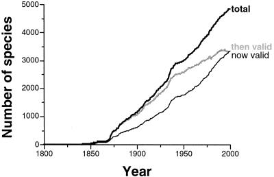
The mammal database makes it possible to reconstruct not just the historical accretion of all names, but the proportion of names known at a time that today are thought to be valid, and even the proportion thought at any time in the past to be valid (Fig. 1). These historical accumulation curves present several key patterns. (i) The intensive exploration of the Western Interior starting around 1868 permanently increased the rate of taxonomic discovery. (ii) Since that time, the rate of description has remained roughly constant at about 35.5 new species per year. There is no correlation between this rate and time in years between 1868 and 2000 [Spearman's rank order correlation r_S = +0.142; t = 1.640; not significant (NS)]. Thus, the accumulation curve is not slowing down, so these data should not be used to extrapolate a total (12). (iii) After an initial burst of synonymizing, the pool of currently accepted names fell to a roughly constant proportion of about three-fifths of all species (bottom line vs. top line, Fig. 1). (iv) By contrast, the proportion of historically recognized names (middle line, Fig. 1) has deteriorated more-or-less steadily and does not appear to be approaching a plateau.

Figure 1.

Growth through historical time in the number of named species of fossil mammals. Thick black line = total number of named species; thick gray line = number of species thought to be valid at a time; thin black line = number of species at a time thought to be valid today.

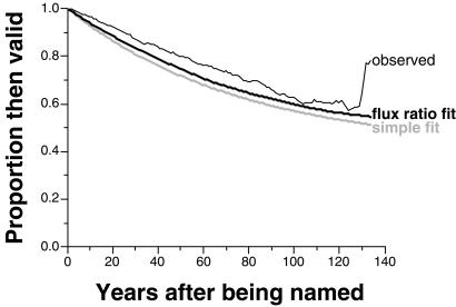
The best way to extract the proportion of truly valid names from these data is to model the proportion of species still recognized a given number of years after being named, i.e., to compute the probability of survival as a function of age (Fig. 2). With infinite research, the curve will approach an equilibrium. Modeling the decline is difficult; extrapolating the equilibrium point by fitting hyperbolic or logistic curves to the data would fail because these parametric extrapolation methods typically estimate equilibria that fall within, or very close to, the existing range of the data (12).

Figure 2.

Historical validity decay curves for named species. Curves show the proportion of all species that were thought to be valid a certain number of years after they were named. Thin black line = observed decay trajectory; thick black line = estimated trajectory based on flux ratio model; thick gray line = estimated trajectory based on simple decay model.

Fortunately, a much simpler and more robust approach can be used instead. This “flux ratio” method can be derived by considering a basic model of the taxonomic revision process. All available names can be divided into changing counts of recognized (X) or unrecognized (Y) taxa. The flux of named taxa from X to Y goes on at some invalidation rate q, and the flux from Y back to X occurs at a revalidation rate r. At first, rate r is irrelevant because all taxa are recognized. However, as rate q operates, the pool of unrecognized taxa grows, so taxa start to move back at rate r. The problem reduces to finding values of X and Y such that Xq = Yr, the equilibrium point at which a proportion X/(X + Y) will be valid. If q and r are known, then because Y = X q/r, X/(X + Y) = X/(X + [X q/r]) = r/(q + r). In other words, the equilibrium proportion of valid taxa is just the flux ratio: the revalidation rate over the sum of the revalidation and invalidation rates. Maximum-likelihood estimates of q and r are simply the numbers of invalidations or revalidations divided by the sums across taxa of the number of years that they have been considered valid or invalid.

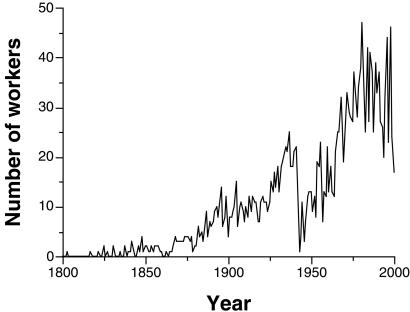
A minor complication is that the mammalian data show a roughly linear decay trajectory (Fig. 2), whereas the flux ratio method in its basic form assumes an exponential, and therefore concave, decay to an equilibrium point. The discrepancy primarily results from the increasing number of active taxonomic workers through historical time (Fig. 3), which has steadily increased the per-year chance that any given species name will be reevaluated. To account for this effect, the time axis is weighted, with the worker-time represented by the ith year being the sum over all species existing after i years of the number of workers who were active i years after each of these species was named.

Figure 3.

Number of taxonomists actively publishing in each historical year. Counts are of taxonomists who published at least one new species name, new genus–species combination, or new hypothesis of synonymy in a given year.

The resulting fitted curve (Fig. 2) is appropriately flattened. Residual discrepancies may result from (i) changes through historical time in the underlying quality of proposed names; (ii) changes in accepted standards for synonymization; (iii) a “grace period” effect whereby names are less often challenged during the careers of the naming authors (16); or (iv) failure to record original papers proposing synonymies, with credited years of synonymization therefore being too young. The first possibility is explored below; untangling the other, apparently minor effects will require additional research.

The flux-ratio estimate of the true proportion of valid species at equilibrium is 50.09%, whereas the current observed proportion is 68.92% (3350/4861). The flux ratio's two-sided 95% confidence interval (CI), easily computed by Monte Carlo simulation, is 47.87–52.16%. If correct, this figure implies that true diversity is 100 (1 − [0.5009/0.6892]) = 27.3% (CI 24.3–30.5%) lower than currently thought, so diversity is overestimated by some 100 (0.6892/0.5009) = 37.6% (CI 32.1–44.0%). This estimate is, if anything, a minimum, because it ignores the fact that some currently invalidated species will be revalidated after much study. Thus, not only would many currently recognized species be removed by a perfect taxonomy, but an additional group of recognized species would have their places taken by revalidated species.

Performance

The flux ratio method assumes that all species are equally subject to invalidation and revalidation, instead of assuming fixed pools of truly valid and invalid species. Does this assumption matter? Fortunately, the question can be answered in the negative by examining a conceptually very different method that does assume completely fixed pools (16). The incorrectly recognized, actually invalid pool of A taxa is modeled as decaying away exponentially at some rate k as taxonomists vet names. Each vetted name moves into the correctly invalidated pool B, whereas a pool of C truly valid taxa remains fixed.

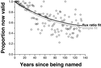
This simple decay method seems to ignore revalidation completely, working only with dates of naming and current validity assessments (Fig. 4). For a given cohort i with N_i taxa all named exactly t years ago, the overall parameters C and k predict specific values of A_i and B_i: for example, A_i + B_i = N − C_i, where N_i is the count of taxa in i and A_i = (N − C_i) e^kt. The probability of obtaining the currently recognized species count X_i = A_i + C_i can be computed by a simple binomial equation; summing the logs of these probabilities across all cohorts yields a log likelihood of C and k. The combination of C and k that yields the highest log likelihood then can be estimated by a grid search.

Figure 4.

Historical validity proportions for cohorts of named species. Points show the proportion of each cohort of species named a certain number of years ago that currently are thought to be valid. Black line = estimated validity proportions based on flux ratio model; gray line = estimated proportions based on simple decay model.

The flux rates also imply a decay function. When a cohort is first named at time 0, all taxa are in X₀, so the rate of decrease in the number of valid taxa is just qX₀ = qN. At this point the simple decay method implies that the same rate is (1 − e^k) (1 − N − C), so q = (1 − e^k) (N − C)/N. By definition, the flux ratio r/(q + r) = C/N. By substituting the expression for q into the left-hand side of this equation, one can show that r = (1 − e^k)C/N.

Therefore, each method employs two free parameters that are algebraically interchangeable and govern formally identical rate-of-change equations. The difference boils down to conceptualization and data. Simple decay assumes steady removal of invalid names until none are left, whereas the flux ratio method assumes a never-ending, two-way flux between pools. Simple decay focuses strictly on the proportions of species in each year cohort that now are valid (Fig. 4); the flux ratio method predicts the validity of all species a given number of years after being named, regardless of whether they were named that number of years before the present or still earlier (Fig. 2).

The fact that both methods maximize likelihoods makes it possible to compare them on equal terms. The log-likelihood of the observed current number of recognized names is 2,723.1 based on the simple decay method, and 2,729.4 (0.2% higher) based on the flux ratios. Because there are 4,861 species, these figures imply that the first method correctly predicts current validity 57.1% of the time, whereas flux ratios succeed 57.0% of the time (see ref. 3 for a similar calculation). Meanwhile, if q and r are the observed coefficients, q′ and r′ are the simple decay method's coefficients, T_X is the grand total number of worker-years that species were valid, and T_Y is the number they were invalid, then the log-likelihood of the invalidation and revalidation outcomes is −[q T_X log q′ + r T_Y log r′ + (1 − q) T_X log (1 − q′) + (1 − r) T_Y log (1 − r′)] = 23,348.7. It is 23,301.7 (0.2% lower) based on the actual flux ratios. These figures each translate into the same average per-worker-year prediction probability of 99.66%.

Nonetheless, the two methods do make very different predictions about the decay process. The flux ratio method implies a truly valid proportion of 47.9–52.2%, whereas the simple decay prediction is merely 40.7%. The predicted proportions of current names that actually are invalid are, respectively, 24.3–30.5% and 40.9%. The observed per-worker-year, per-species flux rates are 3.855e⁻⁴ (q) and 3.869e⁻⁴ (r). With a decay coefficient of −0.013024 and an average of 20.88 worker-years per year across the data set, the simple decay equation implies an invalidation rate q′ of 3.675e⁻⁴, only 4.7% lower—but an revalidation rate r′ of 2.522e⁻⁴, 34.8% lower. Meanwhile, the flux rates imply an initial net rate of decay log{1 − [20.88 q N_t/(N_t − C)]} = k = −0.013667 (4.9% faster), the difference mostly resulting from the larger pool of valid names predicted by the latter method.

The methods also make use of substantively different data (Fig. 2 vs. Fig. 4). In theory, each pattern should exactly reflect the other, because the probability that a species is valid after t years should be independent of whether that species was named t years before the present or earlier. In practice, that assumption clearly is not true, probably thanks to the simple decay method's poor back-estimate of the revalidation rate. In turn, this underestimate stems from the method's sole reliance on counts of currently recognized taxa, which lump together revalidated taxa and unchallenged taxa.

In sum, the flux ratio method uses more data to predict more data, and does a better job of it (Fig. 2). Therefore, with the current data set it seems safest to focus on flux ratios. However, that still leaves the question of why the revalidation rate is underestimated by the simple decay method. One possibility is that the probability of being valid after t years may not be the same for species exactly t years old and still older species—perhaps younger species are more likely to be valid, which also would explain the excessively speedy initial decays implied by both methods (Fig. 2). This hypothesis is tested in the following section.

Trends Through Historical Time

The fact that the underlying quality of newly proposed names does evolve can be shown by breaking down the survivorship data into 27 five-year cohorts between 1850 and 1859, and 1865 and 1989 (Fig. 5). Each includes at least 60,000 species-worker-years of data, with an average of 166 named species and a minimum of 34 named species.

Figure 5.

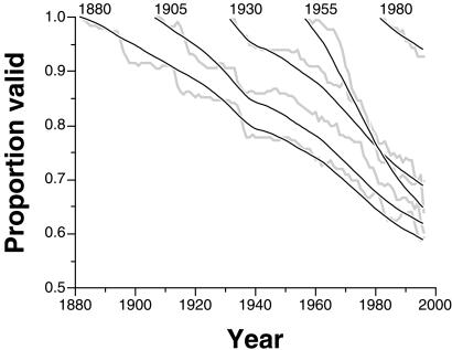
Survivorship curves for 5-year cohorts of species. Curves show changes in the proportion of species of a certain historical age that are thought to be valid. Data are subdivided into cohorts (e.g., the 1880 cohort includes all species named between 1880 and 1884). To avoid clutter, only every fifth cohort is shown. Thick gray lines = observed proportions; thin black lines = flux ratio survivorship estimates.

The decay curves (Fig. 5) show that very young names (e.g., 1980 cohort) decline almost exponentially, and current rates of decline are still steep even in some of the oldest cohorts. Although individual cohorts often show stretches of inactivity or sudden declines, these quirks are minor, and the fitted flux ratio curves (Fig. 5) are generally reasonable. Indeed, the fitted curves even reflect the visible slowdown in taxonomic activity around World War II, where the curves kink in parallel. Of more interest is the dramatic variation in flux ratio coefficients, which generates corresponding variation among cohorts in forecasted equilibrium fractions of valid species. Surprisingly, there is a weak and insignificant correlation between the historical age of a cohort and the flux-ratio-based proportion of truly valid names (n = 27; r_S = +0.311; t = 1.635; NS). High values (>65%) are seen, for example, in the 1855, 1865, and 1915 cohorts; low values (<45%) are seen as late as the 1940, 1950, and 1955 cohorts.

By contrast, younger cohorts consistently have higher proportions of currently accepted names, so there is a strong rank-order correlation between time and the accepted proportion (r_S = +0.654; t = 4.322; P < 0.001). The pattern results from the lack of sufficient time to vet younger names. Despite the trend, the ratio of truly valid to accepted names does not correlate with time (r_S = −0.202; t = 1.032; NS), so new names are only slightly less reliable.

Could variation in both the accepted proportion and the degree of vetting undermine the overall, extrapolated fraction of valid names? This concern can be addressed by summing estimated valid taxon counts across the 27 cohorts. A total of 4,486 of the 4,861 species were named in these intervals, of which 2,992 (66.7%) currently are accepted. The cohort-by-cohort flux ratio analyses (Fig. 5) imply that 2,399 of these species (53.5%) actually are valid, only slightly more than the original flux ratio estimate of 50.1 ± 2.2% for the lumped data set. Thus, the flux ratio method's parameters appear to be robust, even though there has been considerable variation through historical time in taxonomic practice.

Trends Through Evolutionary Time

The results immediately raise serious questions about studies of diversity dynamics in the fossil record. If species counts are inflated, how much can we say about adaptive radiations, equilibrial diversification patterns, and mass extinctions? Seemingly, there are several reasons to not to worry. For example, as-yet-unrecognized invalid species tend to be newly described, used by only a few workers, and known from only a few collections, so they are likely to have short temporal ranges. This tendency actually is a bonus because modern paleobiological studies systematically throw out taxa whose ranges are so short that they are found in only one time interval (3, 4, 18–20). Furthermore, taxonomic revisions over the historical time scale of one or two decades rarely obscure true mass extinctions and long-term diversity trends (13, 15, 21, 22).

Unfortunately, there is a much more pernicious problem: if taxonomic biases change predictably through evolutionary time, then diversity curves, and therefore origination and extinction rates, could be affected in not just absolute but relative terms. This problem can be addressed by splitting the data into million-year cohorts of evolutionary time. Any species ranging into a 1.0 million-year-long bin is included in the bin's cohort. All bins of the Cenozoic save the first are well-sampled enough to do a robust analysis (names in the 65–64 million-years-ago bin have aged for <38,000 worker-years, whereas names in each of the others have aged for >110,000).

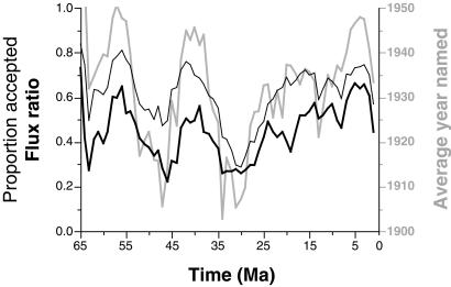
The resulting curves (Fig. 6) show substantial variation and clear temporal trends. All of the curves are strongly autocorrelated at a one-bin lag, making the significance of simple cross-correlations hard to evaluate (mean historical age of names: Spearman's rank-order correlation r_S = +0.812; n = 63; t = 10.874; P < 0.001; proportion of names accepted: r_S = +0.800; t = 10.424; P < 0.001; flux ratio: r_S = +0.844; t = 12.266; P < 0.001). Nonetheless, the cross-correlations are high: bins whose average species names are historically old also have low current rates of acceptance and low flux ratios (mean age vs. acceptance: r_S = +0.875, n = 64; mean age vs. flux ratio: r_S = +0.765).

Figure 6.

Changes in taxonomic quality through evolutionary time. Thin black line = proportion of species names in each 1.0 million-year-long bin that currently are accepted; thick black line = estimated proportion of truly valid names based on flux ratio analysis; thick gray line = average historical year that species falling in each bin were named. Ma, million years.

The two quality measures also track each other (r_S = +0.828), for example, both being consistently low in the mid-Tertiary. However, there are important, lengthy stretches where the flux ratios are even lower, which means that these intervals are very poorly vetted: much of the Paleocene [64–58 million years (Ma)], the mid-Eocene (50–40 Ma), the Eocene–Oligocene transition (36–32 Ma), and the early Miocene (22–17 Ma). Furthermore, taxonomic inflation (the accepted proportion divided by the flux ratio) shows a strong temporal trend (inflation vs. Ma: r_S = +0.557; t = 5.282; P < 0.001), with Paleogene names being consistently unreliable.

Implications for Diversity Dynamics

The inflation ratio can be used to correct published diversity curves (3, 15). However, because the curves are standardized by random subsampling of faunal data (3, 19, 20), they cannot simply be divided by the ratio. The reason is that any junior synonym in the subsample can be discounted only if its senior synonym also has been drawn. The chance of a match is just the ratio s of subsampled to raw, total diversity. If a is the accepted name proportion, f is the flux ratio, and j is the proportion 1,268/1,511 of the invalid names that are junior synonyms (as opposed to nomina dubia), then the proper correction expression is 1 − (1 − j + [j s]) (1 − [f/a]).

However, directly multiplying diversity counts by the correction factors for each bin would not be appropriate because (i) there is no simple way to directly correct turnover rates on the basis of fractional counts; (ii) the counts are of taxa crossing bin boundaries (3, 15, 18–20), not of taxa falling within bins, so corrections applying to individual bins do not apply directly; and (iii) each of the taxa making up a count may itself range across many bins with different correction factors. A better approach is to compute an average correction factor for each taxon across all bins including it in a given subsampling trial, and then weight the taxon by this factor in both diversity counts and turnover rates.

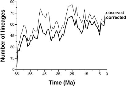
The resulting taxonomic correction (Fig. 7) of the most current sampling standardized curve (3) suggests that Paleogene diversity is consistently lower than Neogene diversity, instead of approximately equal as had been thought. Indeed, the correction significantly raises the slope of a linear regression between time in millions of years and the log of diversity from −0.00647 (SD = 0.00126) to −0.00891 (SD = 0.00123). Possible explanations are the actual existence of two distinct diversity plateaus instead of one, or a lingering geographic bias that inflates the Neogene curve, despite restriction of the data to a circumscribed geographic region (15, 19, 20).

Figure 7.

Correction of the Cenozoic diversity curve for taxonomic bias. Previously published data (thin line), which already are sampling-standardized (3, 15, 19, 20), are revised downwards (thick line) to discount estimated occurrences of hidden invalid names.

Regardless of the reason, the correction makes very little difference in relative terms: the old and new diversity curves are highly correlated (n = 64; r_S = +0.934); instantaneous per-taxon origination rates and extinction rates (see ref. 3 and Fig. 7) are virtually unchanged (origination: means 0.271 and 0.273, r_S = +0.994; extinction: means 0.256 and 0.255, r_S = +0.994); and rates still fall through time (origination vs. time: r_S = +0.423; t = 3.673; P < 0.001; extinction vs. time: r_S = +0.273; t = 2.232; P < 0.05). The rates still are constant during the relatively quiet Eocene–Pleistocene interval (origination: n = 55; r_S = +0.196; t = 1.454; NS; extinction: r_S = +0.120; t = 0.877; NS), during which origination and extinction are still uncorrelated (r_S = −0.064; t = 0.467; NS), and extinction is still uncorrelated with diversity (r_S = −0.011; t = 0.082; NS).

Most importantly, origination rates still fall predictably with rising diversity (r_S = −0.411; t = 3.284; P < 0.01). Negative density dependence of origination rates would cause diversity to fluctuate about a dynamic equilibrium (3, 19, 20). There is a reasonable concern that the correlation might be generated by random sampling error, i.e., by a “regression to the mean” effect that has been shown (23) to severely handicap a closely related and widely used test of population dynamics (24). However, the data already have been corrected for sampling variation (3, 15, 19, 20), rendering this skeptical hypothesis implausible.

In sum, the results do confirm the signature feature of mammalian diversity dynamics: rather than being forced by any extrinsic environmental variables (25), diversity seems to track a dynamic equilibrium (26) that appears to be maintained by density dependence acting on origination rates (3, 19, 20).

Implications for Extant Biodiversity

The general result that fossil diversity is currently overestimated by some 32–44% certainly cannot be dismissed, regardless of its relevance for macroevolutionary theory. Would similar analyses of hyperdiverse living groups yield similarly disturbing proportions of hidden invalid names? Here I argue that a 32% estimate actually would be a conservative lower bound, because our current knowledge of North American fossil mammals is better, not worse, than our knowledge of many living hyperdiverse groups. The comparison is relevant because (i) most extant species are known only from morphological descriptions, (ii) in particular, the taxonomy of extant mammals depends largely on osteological characters commonly preserved in fossils, and (iii) contrary to common perceptions, genetic studies of extant morphospecies with fossil records routinely confirm their status as evolutionary units (e.g., ref. 27).

A key statistic is the proportion of all species that already are known. A reasonable estimate for North American mammals is that 56% of all species that ever existed are known from fossils, or 41% after discounting hidden invalid species. This estimate can be obtained by assuming that a standardized fossil subsample of the extant biota should be proportionate to an identically constructed subsample of the whole fossil record. Let a = the average of 90.7 end-Pleistocene (essentially extant) species appearing in sampling-standardized data (3); b = the 562 end-Pleistocene species, including 53 large mammals that were victims of the anthropogenic end-Pleistocene mass extinction (28) and 509 extant terrestrial North American mammals (29); and c = the average of 965 species appearing in sampling-standardized data for the Cenozoic (3). The sampling-standardized data include a/b = 16.1% of all extant and recently extinct species. If the sampling-standardized data are equally representative of the deeper record and there were x Cenozoic species overall, then a/b = c/x, so x = bc/a = 5,979 species. Because d = 3,350 North American Cenozoic mammalian species now recognized from fossils, 3,350/5,979 = ad/bc = 56.0% of all species have been captured in the fossil record. A strikingly similar figure of 58% has been obtained by using completely different statistical methods involving age-range frequency distributions (30). Assuming that the problem of hidden invalid species affects a, c, and d equally and much more than b, the true proportion may be as low as (100% − 27.3%) × 56.0% = 40.7%.

Analogous estimates for major groups of living species—ignoring the validity problem—are <5% for fungi (31, 32), <10% for coral reef organisms (33), 5–30% for beetles (34), and 37% for hemipterans (35). Living vertebrates are not all that much better known; merely 40–47% of deep-sea fishes have been described (36). Thus, although it might seem that capturing 41% of fossil species is nothing to be proud of, instead this proportion is on the high end of the range for living hyperdiverse groups.

Other facts also suggest that important living groups are remarkably poorly studied, so the fossil mammal data are robust by comparison. Per-species study rates are low for all hyperdiverse groups (6). About half of all living species are known from a single collecting locality (9), but the same figure for North American fossil mammals is merely 29%. Current synonymy rates are only about 20% for insects (9, 16), synonymy rates climb with greater study (Figs. 1–5), and they are higher in very heavily studied groups such as mollusks (38%; ref. 37) and butterflies (>56%; ref. 9). By comparison, the current synonymy rate is 31% for fossil mammal species. Finally, the one other study to estimate a hidden invalid species fraction (16) found that thysanopteran insect diversity might be inflated by 28%, comparable to the 32–44% rate for fossil mammals. Thus, substantial inflation of total species counts should be expected everywhere in the literature on biodiversity. If only 30% of named species are illusions created by unsettled taxonomy, then instead of 5–15 million living species (9, 10), there may be 3.5–10.5 million.

Conclusions

The results yielded by flux ratio analysis show that a disturbingly large proportion of fossil species are likely to be invalid. Surprisingly, however, this strong bias has no great effect on key results concerning diversity dynamics. The results also raise the possibility of substantial taxonomic inflation within poorly studied and diverse extant groups, such as fungi and insects. However, the degree of inflation is small enough to have no major impact on the question of whether a mass extinction is now underway. Despite considerable uncertainties, current estimates suggest that current extinction rates may be two or more orders of magnitude above background extinction and speciation rates (1, 2, 5, 6, 38). If correct, the size of this rate increase dwarfs problems of taxonomic error, regardless of whether synonymy problems are more severe for doomed species. Furthermore, additional bias factors work in the opposite direction: the recent explosion of molecular systematic analyses has made it possible to recognize numerous sibling species, and the application of the phylogenetic species concept also would greatly increase known diversity (39). The challenge of recognizing both sibling species and synonyms in our current taxonomy is clearly enormous, and it emphasizes the profound need for additional funding of primary taxonomic research (6). At current rates of description, we are at least a century away from naming a majority of the Earth's living species (9, 40), much less removing the great empirical barrier of taxonomic uncertainty.

Abbreviations

NS

not significant

Ma

million years

References

- 1.Pimm S L, Russell G J, Gittleman J L, Brooks T M. Science. 1995;269:347–350. doi: 10.1126/science.269.5222.347. [DOI] [PubMed] [Google Scholar]
- 2.Woodruff D S. Proc Natl Acad Sci USA. 2001;98:5471–5476. doi: 10.1073/pnas.101093798. [DOI] [PMC free article] [PubMed] [Google Scholar]
- 3.Alroy J. Paleobiology. 2000;26:707–733. [Google Scholar]
- 4.Foote M. In: Deep Time: Paleobiology's Perspective. Erwin D H, Wing S L, editors. Lawrence, KS: Paleontol. Soc.; 2000. pp. 74–102. [Google Scholar]
- 5.Regan H M, Lupia R, Drinnan A N, Burgman M A. Am Nat. 2001;157:1–10. doi: 10.1086/317005. [DOI] [PubMed] [Google Scholar]
- 6.May R M. Science. 1988;244:1441–1449. doi: 10.1126/science.241.4872.1441. [DOI] [PubMed] [Google Scholar]
- 7.May R M. Philos Trans R Soc London Ser B. 1994;345:13–20. doi: 10.1098/rstb.1994.0082. [DOI] [PubMed] [Google Scholar]
- 8.Hawksworth D L, Kalin-Arroyo M T. In: Global Biodiversity Assessment. Heywood V H, editor. Cambridge, U.K.: Cambridge Univ. Press; 1995. pp. 107–191. [Google Scholar]
- 9.Stork N E. In: Biodiversity II: Understanding and Protecting Our Biological Resources. Reaka-Kudla M L, Wilson D E, Wilson E O, editors. Washington, DC: Joseph Henry Press; 1997. pp. 41–68. [Google Scholar]
- 10.Odegaard F. Biol J Linn Soc. 2000;71:583–597. [Google Scholar]
- 11.Gaston K J, May R M. Nature (London) 1992;356:281–282. [Google Scholar]
- 12.Colwell R K, Coddington J A. Philos Trans R Soc London Ser B. 1994;345:101–118. doi: 10.1098/rstb.1994.0091. [DOI] [PubMed] [Google Scholar]
- 13.Niklas K J, Tiffney B H. Philos Trans R Soc London Ser B. 1994;345:35–44. [Google Scholar]
- 14.Vermeij G J. Malacologia. 1999;41:147–150. [Google Scholar]
- 15.Alroy J. Geology. 2000;28:1023–1026. [Google Scholar]
- 16.Solow A R, Mound L A, Gaston K J. Syst Biol. 1995;44:93–96. [Google Scholar]
- 17.Raup D M. Paleobiology. 1976;2:279–288. [Google Scholar]
- 18.Sepkoski J J., Jr Geol Soc Am Spec Pap. 1990;247:33–44. [Google Scholar]
- 19.Alroy J. Palaeogeogr Palaeoclimatol Palaeoecol. 1996;127:285–311. [Google Scholar]
- 20.Alroy J. In: Biodiversity Dynamics: Turnover of Populations, Taxa, Communities. McKinney M L, Drake J A, editors. New York: Columbia Univ. Press; 1998. pp. 232–287. [Google Scholar]
- 21.Sepkoski J J., Jr Paleobiology. 1993;19:43–51. doi: 10.1017/s0094837300012306. [DOI] [PubMed] [Google Scholar]
- 22.Adrain J M, Westrop S R. Science. 2000;289:110–112. doi: 10.1126/science.289.5476.110. [DOI] [PubMed] [Google Scholar]
- 23.Shenk T M, White G C, Burnham K P. Ecol Monogr. 1998;68:445–463. [Google Scholar]
- 24.Pollard E, Lakhani K H, Rothery P. Ecology. 1987;68:2046–2055. doi: 10.2307/1939895. [DOI] [PubMed] [Google Scholar]
- 25.Alroy J, Koch P L, Zachos J C. In: Deep Time: Paleobiology's Perspective. Erwin D H, Wing S L, editors. Lawrence, KS: Paleontol. Soc.; 2000. pp. 259–288. [Google Scholar]
- 26.Stucky R K. In: Current Mammalogy. Genoways H H, editor. Vol. 2. New York: Plenum; 1990. pp. 375–430. [Google Scholar]
- 27.Marko P B, Jackson J B C. J Paleontol. 2001;75:590–606. [Google Scholar]
- 28.Alroy J. In: Extinctions in Near Time: Causes, Contexts, and Consequences. MacPhee R D E, editor. New York: Kluwer Academic/Plenum; 1999. pp. 105–143. [Google Scholar]
- 29.Cole F R, Reeder D M, Wilson D E. J Mammal. 1994;75:266–276. [Google Scholar]
- 30.Foote M, Raup D M. Paleobiology. 1996;22:121–140. doi: 10.1017/s0094837300016134. [DOI] [PubMed] [Google Scholar]
- 31.Hawksworth D L. Mycol Res. 1991;95:641–655. [Google Scholar]
- 32.Guzman G. Biodivers Conserv. 1998;7:369–384. [Google Scholar]
- 33.Reaka-Kudla M L. In: Biodiversity II: Understanding and Protecting Our Biological Resources. Reaka-Kudla M L, Wilson D E, Wilson E O, editors. Washington, DC: Joseph Henry Press; 1997. pp. 83–108. [Google Scholar]
- 34.Grove S J, Stork N E. Invert Taxonomy. 2000;14:733–739. [Google Scholar]
- 35.Hodkinson I D, Casson D. Biol J Linn Soc. 1991;43:101–109. [Google Scholar]
- 36.Koslow J A, Williams A, Paxton J R. Biodivers Conserv. 1997;6:1523–1532. [Google Scholar]
- 37.Bouchet P. Veliger. 1997;40:1–11. [Google Scholar]
- 38.Sepkoski J J., Jr J Paleont. 1997;71:533–539. doi: 10.1017/s0022336000040026. [DOI] [PubMed] [Google Scholar]
- 39.Knowlton N. Hydrobiologia. 2000;420:73–90. [Google Scholar]
- 40.Erwin T L, Johnson P J. Coleopts Bull. 2000;54:269–278. [Google Scholar]