High-Resolution Multipoint Linkage-Disequilibrium Mapping in the Context of a Human Genome Sequence

Abstract

A new method is presented for fine-scale linkage disequilibrium (LD) mapping of a disease mutation; it uses multiple linked single-nucleotide polymorphisms, restriction-fragment-length polymorphisms, or microsatellite markers and incorporates information from an annotated human genome sequence (HGS) and from a human mutation database. The method takes account of population demographic effects, using Markov chain Monte Carlo methods to integrate over the unknown gene genealogy and gene coalescence times. Information about the relative frequency of disease mutations in exons, introns, and other regions, from mutational databases, as well as assumptions about the completeness of the gene annotation, are used with an annotated HGS, to generate a prior probability that a mutation lies at any particular position in a specified region of the genome. This information is updated with information about mutation location, from LD at a set of linked markers in the region, to generate the posterior probability density of the mutation location. The performance of the method is evaluated by simulation and by analysis of a data set for diastrophic dysplasia (DTD) in Finland. The DTD disease gene has been positionally cloned, so the actual location of the mutation is known and can be compared with the position predicted by our method. For the DTD data, the addition of information from an HGS results in disease-gene localization at a resolution that is much higher than that which would be possible by LD mapping alone. In this case, the gene would be found by sequencing a region ⩽7 kb in size.

Introduction

Methods for mapping disease mutations by the use of family-based linkage analysis have quite low resolution. Even in situations in which hundreds of extended families are available, the methods normally do not provide estimates of map distances at resolutions greater than ∼1 cM (Boehnke 1994). For positional cloning to be practical, a much smaller candidate region is needed, typically ∼0.1 cM (∼100 kb) or less. Linkage disequilibrium (LD) mapping (Bodmer 1986; Lander and Botstein 1986) takes advantage of the fact that the genealogy underlying a sample of chromosomes from unrelated individuals may be very large, incorporating thousands of meiotic events. A disease mutation arises on a chromosome with a specific marker haplotype, and the disease and haplotype are initially associated in a population. Over time, this association decays, because of recombination, with a rate determined by the genetic distances of markers from the disease mutation. Exploiting this relationship, one can use alleles at a linked marker—or haplotypes for several linked markers—from a sample of unrelated affected (and unaffected) individuals, to perform mapping at a resolution much higher than that which is possible by linkage analysis. LD mapping can often reduce the candidate region for a mutation to <0.1 cM, at which point positional cloning is feasible. LD mapping has been widely used for the high-resolution–mapping phase preceding attempts to positionally clone mutations underlying many simple Mendelian disorders, especially in founder populations (reviewed by de la Chapelle and Wright 1998).

A complete, 99.9% accurate, annotated human genome sequence (HGS) will be publicly available within 1–3 years (Lander et al. 2001). For many regions of the genome, an assembled contig, with a complete sequence and a high percentage of genes identified, is available now. Positional cloning is no longer necessary with an HGS in hand, and postgenome mappers will, instead, focus on identification of polymorphisms of genes within a candidate region. This is a much simpler prospect, because even a 1-cM candidate region will contain, on average, only ∼10 genes, given that the entire human genome is ∼3 Gbp (∼3,000 cM) in length and is likely to contain ∼30,000 genes (Lander et al. 2001; Venter et al. 2001). LD mapping methods will remain useful in the postgenome era, however, because, for the mapping of mutations underlying complex disorders, they offer potential advantages over linkage analysis—such as increased power when penetrance is low and a reduced need for extended families—and because they can still greatly reduce the amount of sequence that must be examined in order to identify a mutation. Unlike simple Mendelian diseases, which most often result from nonsense or other mutations that eliminate protein function and that can be readily identified, the mutations underlying complex disorders will most often be missense mutations (the polymorphisms at the apolipoprotein E locus influencing susceptibility to late-onset Alzheimer disease are an example; Corder et al. 1993). Comparisons of frequencies of the mutant and nonmutant sequences in affected and unaffected individuals will be one of the few mechanisms for establishing a role for a polymorphism in disease in these cases and for differentiating between disease-susceptibility polymorphisms and neutral polymorphisms. To do this, a posterior density assigning probabilities to particular exons will be very helpful in reducing the number of polymorphic sites for which frequencies must be compared between the two groups.

Much potential information about the position of a disease mutation is contained in an annotated HGS of a candidate region. This information needs to be effectively incorporated into methods for fine-scale mapping. Exons of genes in a candidate region will have the highest probability of harboring a disease mutation, but mutations may also occur in introns, regulatory sequences, and (with reduced probabilities) nongenic sequences. Nongenic sequences may actually contain undiscovered genes in a poorly annotated genome sequence, and therefore some probability must also be assigned to such regions as possible locations of disease mutations. Prior information about the probability that mutations occur in different regions (introns, exons, etc.) can be obtained from databases of mutations identified in known disease genes. A direct approach for utilizing an HGS in the mapping of disease genes would be to sequentially compare, between affected individuals and control individuals, the sequences of exons, introns, and noncoding DNA in a candidate region, to identify polymorphisms. Although more efficient than positional cloning methods, this approach does not take full advantage of the information available from both an HGS and LD among markers on the sampled chromosomes. In addition to narrowing the candidate region, LD contains potential information about the probability that a mutation lies within any subregion of a candidate region.

In the present study, we develop a Bayesian LD mapping technique that uses information from both an annotated HGS and a dense set of markers that are typed in affected individuals and in normal individuals. An HGS and information (from existing mutation databases) specifying the locations of previously identified disease mutations (in introns, exons, regulatory sequences, etc.) are combined to generate a prior probability distribution for the position of a disease mutation. The method then generates the “posterior” probability distribution for the position of the disease mutation, given both the marker data and prior information from an HGS and mutational databases. The posterior distribution can be used to assign probabilities that particular regions contain the mutation and to decide which regions should be sequenced first in the search for a mutation. The posterior probabilities obtained in this way effectively incorporate information from both the HGS and marker LD. Combining information in such a way can lead to a very efficient localization of the mutation. In the case of the example data analyzed in the present study, it reduced to <7 kb the sequence required for analysis.

One advantage of LD mapping methods for fine-scale mapping in the postgenome era is that the methods may be more robust for the mapping of genes underlying complex genetic diseases, which are typically polygenic and modified by environment. It has recently been suggested that genes underlying these disorders will fall into two classes: (1) genes with small marginal effect and high frequency and (2) genes with large marginal effect and low frequency (Risch 2000). It should be possible to identify the latter by means of essentially classic linkage-mapping approaches (possibly using LD mapping for the final positioning), whereas finding the former will require new mapping strategies. The reason is that a small marginal effect translates to a low penetrance of the disorder and to a high prevalence of phenocopies. Both factors reduce the power of linkage methods. LD mapping offers a potential advantage for the mapping of genes underlying complex diseases, because only affected individuals are included, and the method is therefore insensitive to low penetrance. Reduced penetrance affects only the sampling fraction in an LD mapping study (see Rannala and Slatkin 1998), and this parameter can be shown to have little effect on accuracy. This is a feature that is shared with association studies (e.g., see Risch and Merikangas 1996), although the two approaches are otherwise quite different.

Our simulations (see the “Example: DTD Mutation in Finland” section, below) also suggest that LD mapping can be insensitive to a phenocopy rate as high as 10%. For higher rates, a phenocopy parameter (specifying the probability that a chromosome is not descended from the same disease mutation as are others in the sample) can be included, although we do not attempt to do so here. A second advantage of LD mapping versus linkage mapping, for studies of complex diseases, is that the method potentially can be applied to samples of affected individuals when there is no information on extended families. This is true only if the phase of the haplotypes is known, however. Although information about phase can be obtained by genotyping of relatives (e.g., see Sobel and Lange 1996), the need for extended families in such a procedure eliminates one of the major advantages of LD mapping versus linkage mapping. An alternative approach for establishing the phase is to use information from the same population sample that is used for LD mapping (Clark 1990; Slatkin and Excoffier 1995). If this second strategy is adopted, the additional uncertainty about phase (which may be quite substantial) must be explicitly incorporated into the LD mapping method, to obtain realistic confidence intervals for parameter estimates. This can be done by an extension of the Bayesian approach outlined here, although, in the present study, we consider only the situation in which phase is known.

Exact methods for LD mapping that have been developed thus far have considered only one or two linked markers (Kaplan et al. 1995; Rannala and Slatkin 1998). Extensions to several linked markers (Terwilliger 1995; Xiong and Guo 1997; Graham and Thompson 1998; McPeek and Strahs 1999; Morris et al. 2000) have used simple approximations for either the process of recombination or the underlying genealogical relationships among chromosomes. These approximations assume independence among variables where it does not exist and may perform poorly in some situations (Rannala and Slatkin 2000). Exact multipoint methods that may be used with potentially large numbers of linked markers are needed. It is clear from the results of the present study (and previous analyses) that additional markers can greatly reduce the size of a candidate region. LD mapping methods also must be extended to explicitly model allelic and locus heterogeneity, phenocopy, and population substructure. To account for all of the potential problems arising for complex diseases and samples of individuals from heterogeneous populations, as well as to allow an annotated HGS to be incorporated into LD mapping, a very general and readily extendable numerical framework is needed. In the present study, we develop a new method for multipoint LD mapping, using numerical Markov chain Monte Carlo (MCMC) techniques that offer much flexibility. With this framework, it is possible to incorporate additional parameters and genetic models that are more elaborate.

The Bayesian MCMC approach developed here allows calculation of posterior probabilities by numerically intensive methods and does not rely on the composite likelihood (or other) approximations employed in previous methods. In particular, it explicitly integrates over gene trees, avoiding the composite-likelihood approximation, for the underlying gene tree, that is used by McPeek and Strahs (1999) and Morris et al. (2000). Our method offers several potential advantages over existing methods: information from an annotated HGS and a mutational database can be readily incorporated into a LD mapping study; more-realistic models that integrate over uncertainties about the values of nuisance parameters such as the population growth rate can be used; and, potentially, genotypes—instead of haplotypes—can be used, by treating the haplotypes as unobserved random variables and by implementing a likelihood similar to that considered by Slatkin and Excoffier (1995), thus eliminating the need for extended families.

In the present study, we depart from traditional statistical approaches used in linkage mapping, which have relied mainly on the method of maximum likelihood. Instead, we develop a Bayesian LD mapping method that generates the posterior density of the map position of a disease mutation, relative to a set of linked markers. The method leads to an easily interpretable measure of uncertainty for parameter values and can be extended to simultaneously predict both the genetic model (incorporating potential allelic or locus heterogeneity) and the parameter values, although we do not do so here. In the present study, we focus on (a) developing the general theory underlying our method and (b) implementing the method in a computer program. The principal innovation is the explicit incorporation of an annotated HGS into LD mapping.

Theory

Let X={X_ij} be a matrix of multilocus haplotypes for n chromosomes sampled from unrelated individuals affected with a particular genetic disorder. It is assumed that each chromosome carries the disease mutation, although this assumption can be relaxed. Each chromosome is typed for L markers, where X_ij is the marker allele present at locus j on chromosome i. We define X_i to be the multilocus haplotype of the ith chromosome. It is assumed that, in its recent history, the population from which the chromosomes are sampled has experienced exponential growth (or decline) with rate ξ. If ξ=0, then the population size has remained constant. Other demographic models can be incorporated easily. Consider a disease mutation that first arose at time t₀ in the past, where time is measured in generations. Define f to be the fraction of the total population of present-day disease chromosomes (descended from this initial mutant) that are sampled. For convenience, we define Λ={f,ξ,t₀} to be a vector containing the demographic parameters of the model.

Let Y₀ be the multilocus haplotype present on the chromosome on which the disease mutation first arose. Let p={p_ij} be a matrix of the allele frequencies on normal chromosomes, where p_ij is the frequency of allele i at locus j. The gene tree underlying the sample of chromosomes describes the sample's history with respect to the disease locus and is represented as τ={T,t}, where this is a vector of the labeled binary tree T with tips i=1,2,…,n (representing the sampled chromosomes) and nodes i=n,n-1,…,2, representing the n-1 times, in the past, at which the lineages arose from common ancestral chromosomes. The times at which these shared ancestors (nodes) existed are referred to as the “coalescence times” and are represented by t={t_i} for all i=n,n-1,…,2, where t_i is the time, in the past, at which i mutant lineages coalesced to i-1 ancestral lineages.

A gene tree and the coalescence times on that tree are illustrated in figure 1. We follow the approach of Rannala and Slatkin (1998) and employ the intra-allelic coalescent of a rare mutation, to determine the probability distribution of coalescence times and gene trees in our analysis. Other coalescent models could also be used in the same general framework. Let Y={Y_ij} be a matrix of the n-1 (unobserved) haplotypes found on the ancestral chromosomes at each node in the gene tree, where i=n,n-1,…,2. The ith ancestral haplotype is associated with the ith internal node of the gene tree and with the ith coalescence time. The L-1 map distances between markers are assumed to be known and are represented by d={d_j}, for j=2,3,…,L, where d_j is the map distance between markers j-1 and j. We define θ to be the map distance between marker allele 1 and a disease mutation M. The parameter θ is of specific interest for gene mapping: if θ<0, then the mutation lies to the left of marker 1; if θ>Σd_i, it lies to the right of all the markers (see fig. 2). The symbol Ω denotes an annotated HGS spanning a region that extends some distance beyond both marker 1 and marker L; this provides some of the data for the analysis. The parameters and observed variables are summarized in table 1.

Figure 1.

Two hypothetical gene trees underlying a sample of five disease chromosomes, illustrating the coalescent times t and the tree topology T. The parameters denoted as t₅, t₄, t₃, and t₂ represent the times, in the past, when chromosomes have coalesced to, respectively, four, three, two, and one ancestral chromosome. The parameter t₀ is the time when the mutation first arose. The gene trees shown on the left and right have different values for T but identical values for t. T and t are independent parameters.

Figure 2.

Three chromosomes typed for four marker loci, illustrating the relationship between the map distances of the markers, d={d₂,d₃,d₄}, and the disease-mutation location θ. In panel A, the mutation is to the left of all the markers; in panel B, it is to the right of all the markers; in panel C, it is flanked by markers to the left and markers to the right. The disease mutation is represented as an ellipse and is represented by “M” in panel A; the markers are represenetd as rectangles and are labeled as “1”–”4” in panel A.

Table 1.

Definitions of Parameters of MCMC LD-Mapping Method

Parametera	Description
Known:
X={Xij}	Multilocus haplotypes on the n sampled disease chromosomes that are typed for L markers, where Xij is the marker allele present at locus j on chromosome i
∧={f,ξ,t0}	Demographic parameters, where f is the fraction of the total population of disease chromosomes included in the sample, ξ is the population growth rate, and t0 is the age of the mutation
p={pij}	Marker-allele frequencies in the population of normal chromosomes, where pij is the frequency of allele i at locus j
d={dj}	The L-1 map distances between markers, where dj is the map distance between markers j-1 and j
Ω	Annotated HGS spanning a region that extends some distance beyond both markers 1 and L
Unknown:
Y0={Yj}	Multilocus haplotype present on the chromosome on which the disease mutation first arose, where Yj is the marker allele at the jth locus
Y={Yij}	Ancestral haplotypes that existed on the n-1 internal nodes of the gene tree, where Yij is the marker allele present at the jth locus of the ith ancestral node
θ	Position of the disease mutation (in map units) relative to marker locus 1
τ={T,t}	Gene tree T of the n disease chromosomes and the n-1 coalescence times t={ti} (i=2,3,…,n-1), where ti is the time at which i chromosomes coalesce to i-1 ancestors

^aParameters that are assumed to be known a priori and parameters that are estimated by the algorithm are categorized as known parameters and unknown parameters, respectively.

The Posterior Distribution of Parameters

In the present study, a Bayesian multipoint LD mapping method is developed that is based on the following probability-density function

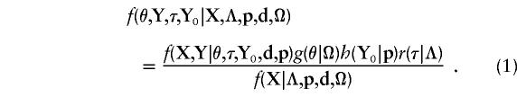The first term in the numerator of equation (1) is the likelihood. The remaining terms in the numerator are prior probability distributions for each of the parameters. By evaluating integrals and sums over the variables of equation (1), we can obtain the marginal density of any of the parameters θ, Y, τ, or Y ₀ that happen to be of interest. In practice, the marginal densities are not easily obtainable by analytical approaches, and we develop instead an MCMC method to obtain these marginal posterior probabilities. In particular, we will focus on the marginal posterior probability density of θ, represented by f(θ|X,Λ,p,d,Ω), which can be used to localize a mutation relative to the marker loci and the gene sequence.

We implement the Metropolis-Hastings (MH) algorithm (Metropolis et al. 1953; Hastings 1970) in our method. Related approaches have been used to estimate population demographic parameters (such as the effective population size) from a sample of DNA sequences, by use of likelihood-based approaches under a Kingman (1982) coalescent model of population genealogy (Kuhner et al. 1995), and to obtain marginal probabilities of phylogenetic trees (Yang and Rannala 1997; Larget and Simon 1999). Recently, Morris at al. (2000) presented a Bayesian MCMC method for LD mapping, calculating the posterior densities of θ and other model parameters. Their method differs from ours in several ways. The most significant differences are that they used a composite likelihood approximation (equivalent to assuming that the gene tree is a star genealogy), rather than integrating over τ, and, for θ, they used a uniform prior that did not incorporate prior information from an HGS.

Prior Distributions of Parameters

Prior probability distributions for the parameters Y₀, τ, and θ are needed to evaluate the numerator in equation (1). Following the suggestion by Terwilliger (1995), we used the observed frequencies of marker alleles on normal chromosomes, p, as the prior h(Y₀|p) for the probability distribution of marker haplotypes on the ancestral chromosome on which the mutation first arose, Y₀. For simplicity, we ignore uncertainties about p that arise because p is estimated from a population sample of chromosomes from normal individuals. This additional source of uncertainty can be easily taken into account by using a Dirichlet prior to model the probability density of p, given the population sample of chromosomes (e.g., see Rannala and Mountain 1997). The probability distribution of τ is based on Rannala and Slatkin's (1998) coalescent model for a rare mutation and is completely determined by the demographic parameters Λ.

We considered two possible prior probability distributions for θ . The first assumes no prior information and gives uniform probabilities to all possible θ values within a specified interval; this is the prior used by Morris et al. (2000). The second prior incorporates information from an annotated HGS. In this case, we used the observed distribution of mutations (among introns, exons, and regulatory regions) in a database of the spectrum of point mutations observed in previously identified disease genes. The disease genes that we used to establish the prior probability that the mutation resided in any given region based on an annotated HGS were those in the Human Gene Mutation Database Cardiff. Probabilities were derived from the statistics page on this web site, which includes all known point mutations in the database. Probabilities were also obtained by counting the types of mutations observed in a dozen randomly chosen disease genes from several specialized databases, and the numbers obtained were very similar to those observed in the totals in the Human Gene Mutation Database Cardiff.

If there are Z introns, exons, and either regulatory or nongenic sequences, the candidate region is divided into Z segments. The probability density of the mutation position at point z_i in the ith segment is

Because this prior probability will always occur in a ratio in the MH algorithm (see the “MH Algorithm” section of the Appendix), the equation simplifies to a ratio of the relative mutation probabilities for the segments being considered as potential positions for the mutation. Models with more detail could be used, weighting nucleotides differently according to the expected rates of transition versus transversion, the codon-specific probabilities of synonymous versus nonsynonymous mutations at particular sites, etc. Although coarse, the categories that we consider in determining the prior are likely to be the ones having greatest effect. It is probably still worthwhile to consider models with more detail and additional categories, but their effects on the prior are likely be small.

Bayesian Inference of the Disease-Mutation Location

To obtain point estimates and confidence intervals for parameters, we generated the posterior distributions of θ, τ, Y, and Y₀, using the MH algorithm (Metropolis et al. 1953; Hastings 1970). In the present study, we focused on estimating the value of θ (the position of the disease mutation relative to marker 1) and obtaining a confidence interval for this estimate. The posterior distribution of θ was obtained by running the MCMC program and sampling the value of θ at each iteration (after burn-in sufficient to allow the chain to reach a stationary distribution). The frequency histogram of the values of θ (for bins of equal width) observed in the chain approximates the posterior probability that the true value of θ is contained within a particular range. The mode of the posterior distribution was estimated as the interval within which θ was contained with the highest frequency; this was taken as the best estimate of the true value of θ.

The α-percent credible set of values for θ (a Bayesian quantity analogous to the classic 95% confidence interval [95%CI]) was obtained by successively adding intervals, in rank order, to the credible set, according to the frequency at which θ was observed in the interval, until the sum of the relative frequencies in the included intervals exceeded α. The credible set of regions obtained in this way need not be contiguous and may contain several disjoint regions in which the mutation is likely to reside. Mathematical details of the likelihood calculation for evaluation of the numerator of equation (1) and of the implementation of MCMC to obtain the marginal posterior probabilities are given in the Appendix.

Example: DTD Mutation in Finland

DTD is an autosomal recessive disease whose main characteristics are dwarfism and generalized joint dysplasia. DTD is present at a high frequency in the Finnish population (1%–2% are carriers), presumably because of a founder event. This population is thought to have derived largely from a small founder population ∼2,000 years ago (∼100 generations). Linkage analysis of Finnish pedigrees initially isolated the disease gene to a region spanning ∼2 cM on chromosome 5q31-q34 (Hästbacka et al. 1990). Its predicted location was further refined by Hästbacka et al. (1992), who used an LD technique based on Luria and Delbruck’s (1943) analysis of mutation in bacterial populations. Positional cloning subsequently showed that the location predicted on the basis of LD mapping was very accurate (Hästbacka et al. 1994).

The gene containing the DTD mutation is known as “SLC26A2” (solute carrier family 26 [sulfate transporter]), or DTDST, and is located ∼70 kb proximal to the CSF1R (colony-stimulating factor 1 receptor) gene. The main mutation, present in ∼90% of Finnish disease chromosomes, is a GT→GC transition in a 5′ UTR exon of SLC26A2 (Hästbacka et al. 1999), which results in decreased levels of mRNA. DTD in the Finnish population has been used to test several other LD methods (e.g., see Kaplan et al. 1995; Graham and Thompson 1998; Rannala and Slatkin 1998). With our MCMC, we used the same data set to test the predicted mutation location. The demographic parameters that we used in our analysis were identical to those used by Rannala and Slatkin (1998).

The haplotype frequencies used in our analysis are from table 2 in an article by Hästbacka et al. (1992), supplemented by unpublished data from J. Hästbacka. Five markers were used, spanning an ∼20-kb region within the CSF1R gene. The relative positions of the markers, the surrounding genes, and the DTD mutation are shown in figure 3. These markers include two RFLPs—labeled “EcoRI” and “StyI” in figure 3—and three microsatellites—labeled “TAGA,” “CCTT,” and “CA.” The RFLPs are diallelic, and the microsatellite alleles were dichotomized according to (presumed) ancestral versus nonancestral alleles. The 148 disease chromosomes in the data set include 11 distinct haplotypes, the most prevalent of which constitutes ∼53% of the sample. On the basis of the allele frequencies observed in a sample of normal chromosomes, this haplotype would be present at a frequency of only 6.2×10^-5, at linkage equilibrium. The method presented in the present study assumes linkage equilibrium among markers on normal chromosomes, although this assumption can be relaxed. A χ² test of linkage equilibrium for the sample of normal chromosomes from the data reported by Hästbacka et al. (1992) was not significant, suggesting that the assumption is valid for these data.

Figure 3.

Distribution of exons, introns, and regulatory and nongenic sequences in a 400-kb region, of chromosome 5, surrounding the SLC26A2 gene that contains the DTD mutation. Exons are indicated by vertical lines, introns by the thick unbroken horizontal lines, and both regulatory and nongenic regions by dotted horizontal lines. Both the scale of the physical distance (top) and the scale of map distance (bottom), which is inferred from the physical distance (under the assumption that 1 cM = 1 Mb), are shown. The six genes identified in this region—PDE6A, SLC26A2, CSF1R, PDGFRB, CDX1, and SLC6A7—are indicated below the gene diagram. The positions of the five markers—EcoRI, TAGA, StyI, CA, and CCTT—in the CSF1R gene are indicated by labeled arrows, as is the exon of the SLC26A2 gene containing the DTD mutation.

In recoding the microsatellites as biallelic, by pooling alleles into two categories, we assumed that, in the founder population, the DTD mutation was present only on this haplotype. However, we also allowed for other potential ancestral haplotypes (using, for the ancestral haplotype, a prior distribution based on the observed marker-allele frequencies on normal chromosomes) in our analysis. We tried the analyses by either using the prior (described above) based on the marker frequencies on normal chromosomes or conditioning on the ancestral haplotype as being the most common haplotype on disease chromosomes; the resulting posterior densities were essentially identical. We have summarized the frequencies of the five haplotypes (with data recoded as binary) present on disease chromosomes, for the data reported by Hästbacka et al. (1992), and these are shown in table 2.

Table 2.

Frequency of Marker Haplotypes on Disease Chromosomes^[Note]

No. of Copies	EcoRI	TAGA	StyI	CA	CCTT
	Haplotypea
137	0	0	0	0	0
6	0	1	1	1	0
3	0	1	1	0	0
1	0	0	0	1	0
1	1	0	0	1	0
	p0b
	.088	.361	.256	.161	.049

Note.— Data are those reported by Hästbacka et al. (1992) and include unpublished frequencies provided to the authors by J. Hästbacka.

^aOnly the putative ancestral (represented by 0) and derived (represenetd by 1) alleles are shown.

^bFrequency of ancestral allele at each locus in the sample of normal individuals.

Weights for the sequence-based prior were chosen on the basis of the frequencies, of known point mutations, recorded at the Human Gene Mutation Database Cardiff. The most recent statistics available for the database give relative frequencies of 1.0 for missense/nonsense mutations, .17 for splicing mutations, and .01 for regulatory mutations; for the purposes of our method, we categorize these weights as exonic, intronic, and nonexonic/nonintronic, respectively; for the MCMC results reported in the present study, we have used relative weights of 1.0, .17, and .02, respectively, for these three categories. The addition of weight to the nonexonic/nonintronic region accounts for the possibility that there are genes in the region that have not yet been discovered. The amount of weight added to this category should reflect one’s confidence in the completeness of the annotation in the region of interest.

The basic program requires that distances between the markers be expressed in map units (1% recombination = 1 cM). If a sequence-based prior is to be used, the relative positions of the markers and of the exon/intron boundaries are required for all genes in the region of interest. Among different databases, there are often considerable differences between the exon numbers and locations. For consistency, we used the current (as of February 28, 2001) GenBank database, for all relative distances. Physical distances were converted to map units by assuming that 1 cM = 1 Mb. Alternatively, one could use data from a linkage (or radiation hybrid) map, to predict map distances directly.

Figure 4 shows the posterior probability distribution of the distance (in map units), represented by θ, from marker 1 of the DTD mutation, for the data reported by Hästbacka et al. (1992) and estimated by MCMC using either a prior probability density derived from an annotated HGS for this region or a uniform prior. The positions of exons, introns, and regulatory or nongenic sequences (on the basis of a physical map and a scale of 1 cM = 1 Mb) are shown at the top of figure 4. The 95% credible set for both analyses (HGS prior and uniform prior) is defined by the regions extending above the dotted horizontal line at the bottom of figure 4. In both analyses (HGS prior and uniform prior), the greatest posterior probability was to the left of (i.e., centromeric to) the markers. This is the actual relative position of the mutation. Although this was true for our analysis of the five markers, an analysis of only the single marker (i.e., EcoRI) analyzed by Rannala and Slatkin (1998) placed equal probability to the left and right of the marker when it was used with a uniform prior for θ, although it still correctly placed more probability to the left when it was used together with an HGS prior (fig. 5). The four additional markers improve the estimate substantially in this case, reducing the size of the 95% credible set of values both when an HGS prior is used and when it is not (compare figs. 4 and 5). This is despite the fact that all the additional markers are in a relatively small region (within the CSF1R gene). For the analysis using all five markers, the 95% credible set for the case in which an HGS prior is used is ∼86% of the width of the credible set obtained with a uniform prior.

Figure 4.

Posterior probability distribution of θ, generated by application of the MCMC algorithm to the data reported by Hästbacka et al. (1992), for five markers—EcoRI, TAGA, StyI, CA, and CCTT—when, for θ, either a uniform prior probability distribution (black line) or a prior distribution based on an HGS (gray bars) was used. Exons are indicated by vertical lines, introns by the thick unbroken horizontal lines, and both regulatory and nongenic regions by dotted horizontal lines at the top of the figure. The dotted horizontal line near the bottom of the figure indicates the cutoff for intervals to be included in the Bayesian 95% credible set of values for either posterior distribution. Proportions exceeding this cutoff are included in the credible set (analogous to the classic 95%CI). The mode (i.e., the most probable interval) and the second most probable interval of the posterior distribution, obtained by use of an HGS, together contain ∼22% of the iterations of the MCMC and cover a 7-kb region that includes the exon containing the DTD mutation.

Figure 5.

Posterior probability distribution of θ, generated by application of the MCMC algorithm to the data reported by Hästbacka et al. (1992), for one marker—EcoRI, when, for θ, either a uniform prior probability distribution (black line) or a prior distribution based on an HGS (gray bars) is used. Exons are indicated by vertical lines, introns by the thick unbroken horizontal lines, and both regulatory and nongenic regions by dotted horizontal lines at the top of the figure. The dotted horizontal line near the bottom of the figure indicates the cutoff for intervals to be included in the Bayesian 95% credible set of values for either posterior distribution. Proportions exceeding this cutoff are included in the credible set (analogous to the classic 95%CI). The mode (i.e., the most probable interval) and the second most probable interval of the posterior distribution, obtained by use of an HGS, together contain ∼11% of the iterations of the MCMC and cover a 7-kb region that includes the exon containing the DTD mutation.

For the five-marker analysis, the two histogram bars spanning the area from −.080 to −.087 cM contain the largest proportion (∼22%) of iterations and also contain the DTD mutation (when a relationship of 1 cM = 1 Mb is used to translate the physical map into the genetic map). A rational approach in searching for mutations by using posterior probabilities is to sequentially sequence regions corresponding to the histogram bars, taken in rank order, containing the greatest proportion of iterations from the MCMC run. Following that approach, we would, in this case, need to sequence <7 kb in order to find the mutation. When only the EcoRI marker was used (fig. 5), ∼11% of the iterations were contained in the two histogram bars comprising the largest proportion of iterations, and these spanned an ∼7-kb interval that contained the exon carrying the DTD mutation. Thus, including the four additional markers approximately doubled the posterior probability of this mutation-containing region. On average, for the five-marker analysis, use of an HGS prior would, ∼50% of the time, require examination of 39% as much sequence as would be required when a uniform prior was used (i.e., the 50% credible set is ∼39% as wide for an HGS prior as it is for a uniform prior).

Simulation was also used to evaluate the performance of the method for the conditions found for the DTD mutation in Finland. Using identical values for the demographic parameters and the position of the DTD gene mutation in the human genome, we simulated an identical number of disease chromosomes by first simulating the gene tree and coalescence times and then simulating chromosomes under the specified recombination process on the gene tree. In the simulation of chromosomes by recombination on the gene tree, it was assumed that recombination events in the ancestry of the sampled chromosomes occurred only in heterozygotes (as assumed in the model used to derive the transition probabilities); it was also assumed that the recombination rates corresponded exactly to those predicted by the physical map with 1 cM = 1 Mb. The data generated in the simulation was analyzed by our MCMC program, under the assumption that the position of the disease mutation was unknown.

The results of the analysis of the simulated data are shown in figure 6. The posterior density is very similar to that obtained in our analysis of the original data, except that (a) a greater proportion of iterations were contained in the region surrounding the actual position of the mutation (when the HGS prior was used) and (b) a greater proportion of iterations were to the left of the markers (the actual position relative to the markers), both with and without an HGS prior. The two histogram bars containing the most iterations (see fig. 6) contained 34.5% of the total iterations and spanned a region of ∼7 kb that contained the exon carrying the DTD mutation. The higher posterior probabilities, in this case, may reflect the fact that the demographic parameters were known with absolute certainty for the simulated data but not for the actual data. This could cause lower posterior probabilities for the actual data, reflecting a poorer fit of the data to the model.

Figure 6.

Posterior probability distribution of θ, generated by application of the MCMC algorithm to the simulated data, for five markers—EcoRI, TAGA, StyI, CA, and CCTT—located at positions in the genome that are identical to the original marker positions reported by Hästbacka et al. (1992), when, for θ, either a uniform prior probability distribution (black line) or a prior distribution based on an HGS (gray bars) is used. The sample sizes and the demographic parameters used to simulate the data are identical to those used for analysis of the data reported by Hästbacka et al. (1992), and the mutation is assumed to be in the same location. Exons are indicated by vertical lines, introns by the thick unbroken horizontal lines, and both regulatory and nongenic regions by dotted horizontal lines at the top of the figure. The dotted horizontal line near the bottom of the figure indicates the cutoff for intervals to be included in the Bayesian 95% credible set of values for either posterior distribution. Proportions exceeding this cutoff are included in the credible set (analogous to the classic 95%CI). The mode (i.e., the most probable interval) and the second most probable interval of the posterior distribution, obtained by use of an HGS, together contain ∼35% of the iterations of the MCMC and cover a 7-kb region that includes the exon containing the DTD mutation.

Simulations were also used to evaluate the sensitivity of the results to either potential locus heterogeneity or phenocopies (both of which can be expected to occur in complex genetic disease). In these simulations, demographic and genetic conditions were again assumed to be identical to those reported by Hästbacka et al. (1992), except that 10% of the “disease” chromosomes were actually drawn from the population of normal chromosomes. This phenocopy rate had little effect on the posterior probabilities of disease-mutation location. The two histogram bins containing the highest posterior probabilities, in this case, spanned the interval from −.82 to −.85 cM, which differs only slightly from the interval of −.80 to −.87 cM, which is spanned by these two bins for the original data.

If an annotated HGS is available, as well as a large number of mapped polymorphic marker loci (e.g., single-nucleotide polymorphisms), this will influence the choice of marker locations. In fact, markers could conceivably be chosen in a way that would optimize the resolution of an LD mapping study. The markers used by Hästbacka et al. (1992) are probably in a region more confined than that which would be used in a contemporary study. We examined the effect of marker location on the posterior distribution of disease location, by again simulating the data under conditions identical to those used by Hästbacka et al. (1992), but with markers positioned uniformly over the interval from −.4 to .4 cM. Marker position has a large effect on the posterior probability in this case, significantly improving the localization of the mutation. The two histogram bins containing the highest posterior probability accounted for 34.5% of the probability in simulations with markers in their original positions, but, for the simulated data with uniformly spaced markers, this probability increased to 60.4%. The width of the 95% credible set also decreased dramatically.

Another potential impact of the prior is on the rate of convergence characteristic of the MCMC algorithm. We used the approach of Gelman (1996), which compares between-chain and within-chain variances, to diagnose convergence (see the Appendix). A more informative prior might be expected to increase the rate of convergence, since it causes the chain to spend more time in regions of high posterior probability. Figure 7 shows the log-likelihood and the value of (defined in the Appendix) at each of 150,000 iterations for a run with two simultaneous chains analyzing the data reported by Hästbacka et al. (1992), both with and without an HGS prior. There is little difference between the convergence rates of the two runs: at 150,000 iterations, the run with an HGS prior has a value of whereas the run with a uniform prior has a value of , indicating that neither chain has converged. Both chains appear to converge after ∼500,000 iterations (not shown), at which point , and that was the number of iterations used for our burn-in period.

Figure 7.

Log-likelihood and value of statistic (both defined in the Appendix), at each iteration of the chain in two MCMC runs analyzing the data reported by Hästbacka et al. (1992), for five marker loci. The two runs are shown separately, as black and gray lines, in the upper and lower panels. The upper panel shows the result when an HGS prior is used, and the lower panel shows the result when a uniform prior is used. To diagnose convergence, each run actually included two chains running in parallel. Similar log-likelihoods and a value of approaching 1.001 indicate convergence of the chains. In this case, the chains do not converge after 150,000 iterations but do converge after 500,000 iterations. Comparison of the two panels shows that there appears to be little difference, in the rate of convergence, between the chains run with an HGS prior and the chains run without an HGS prior.

Discussion

In the present study, we have developed, for high-resolution multipoint LD mapping, a new method that uses information from both the LD observed among multiple markers in a sample of disease chromosomes and an annotated HGS. Incorporating information about the distribution of exons, introns, and either regulatory or nongenic sequences in a candidate region can greatly reduce the extent of the credible set of values for θ, as can the inclusion of additional marker loci in the region. Surprisingly, the addition of markers in a region appears to improve estimates of disease location even if the additional markers are quite close to one another and all are either telomeric or centromeric to the disease mutation. Presumably, this is because the tendency of recombination events to occur with increased frequency at markers most distal to the disease mutation conveys significant information about location. For example, in the case of the Hästbacka et al. (1992) data that we analyzed, all markers were positioned within a relatively small region telomeric to the DTD mutation, yet additional markers further refine the estimated location of the DTD mutation, compared with the estimate based on a single marker (i.e., EcoRI). Other simulations, not presented here, suggest that, in the case of a uniform prior for θ, the posterior probability density of θ undergoes a quantitative change from a bimodal distribution (when either the markers are either all telomeric or all centromeric to the mutation) to a unimodal distribution (when markers flank both sides of the mutation). Thus, the relative shape of the posterior distribution may also convey information, at a gross level, about the markers' positions relative to the position of a mutation. Possibly, one could exploit this positional effect to develop a method for testing the hypothesis that a set of markers flank a mutation (or are, instead, either all telomeric or all centromeric to it), to guide researchers in choosing additional markers in narrowing the candidate region.

Bayesian posterior probabilities can be used in various ways once they have been estimated for a set of data; for example, the probability that a mutation lies between any pair of markers i and j (given that it is located somewhere in the prespecified interval used for the MCMC analysis) is simply the frequency of values of θ in the region D_i<θ<D_j in the MCMC run, where D_i is the position of marker locus i relative to marker locus 1 (see the Appendix). In addition to their use in predicting either the relative or the absolute location for θ, the posterior probabilities can be directly incorporated into the final sequencing phase of a gene-mapping study. By rank-ordering intervals according to the frequency with which θ is observed in each interval in the MCMC run, one can, in searching for a gene, successively sequence each interval, from most probable to least probable. This is expected to be much more efficient than simply beginning at the mode (of either the likelihood or the posterior probability distribution) and sequencing regions while moving outward from the mode. In many cases, with multiple loci and an HGS prior, the posterior density will be multimodal, and the most efficient approach for finding the disease mutation will be to sequence several disjunct regions. Sequencing the rank-ordered intervals from the posterior density, as suggested in the present study, seems to be an optimal solution when several different regions are all likely locations.

Another innovation made possible by a Bayesian approach to high-resolution mapping is an analysis of the projected cost of finding the gene if sequencing is initiated with use of the existing posterior probability distribution is used. This is a straightforward application of decision theory (e.g., see Berger 1985). If, in a sample of disease chromosomes and normal chromosomes, intervals are sequenced in rank order according to their posterior possibilities, the expected cost in finding the gene is

where E is the expectation, Θ is the number of intervals into which the data from the MCMC analysis have been binned, C(z_i) is the expected cost of sequencing the ith interval, z_i, for a sample of disease chromosomes and normal chromosomes, and f(θ∈i|X,Ω,Φ) is the estimated posterior probability that the mutation lies in the ith interval, given the haplotype data X, the HGS data Ω, and the remaining parameters (Λ, p, etc.), which collectively are represented by Φ. If the expected cost remains high, one could consider sampling either additional disease chromosomes or additional markers, to attempt to further refine the posterior probability density before initiating the sequencing phase of the project.

Because disease chromosomes are not independent random variables (in that they are related by a common underlying genealogy), it is not obvious that the sampling of additional disease chromosomes will have a large effect on the posterior distribution of the mutation location. We investigated the effects of sampling in the Hästbacka et al. (1992) study by performing the analysis on random subsamples of disease chromosomes from the original data. We generated the posterior distribution for subsamples of 25, 50, and 100 disease chromosomes. For the complete sample of 148 chromosomes, the proportion of observations in the two histogram bins with highest posterior probability was 22%, whereas, for the subsamples, the corresponding proportions were 9.4% (25), 8.3% (50), and 12.4% (100). Similarly, the total width of the 95% credible set was 0.21 cM for the complete sample of 148 chromosomes, whereas for the subsamples the corresponding widths were 0.62 cM (25), 0.28 cM (50), and 0.27 cM (100). It is clear from these results that increasing the sample size even to >100 continues to have an important effect in narrowing the possible position of the disease mutation. The effect of sampling additional marker loci needs to be carefully studied before any general conclusions are reached; intuitively, one would expect that increasing the density beyond some threshold would provide diminishing returns, since few or no recombination events will have occurred between nearby markers in the sample. Simulations suggest that the computing time increases as an approximately linear function of the number of marker loci. On a 1-Ghz Pentium III computer, the five-marker Hästbacka et al. (1992) data required ∼4 h of computing time, suggesting that analyses of up to ⩾20 marker loci should be feasible, even for relatively large samples of ⩾100 disease chromosomes.

The Bayesian approach developed here can also be readily extended to allow allelic and locus heterogeneity, by integrating over different genetic models. It may even be possible to consider models with more than one disease locus in a population (a consideration particularly important for studies of complex genetic diseases), although this will obviously reduce the power and necessitate a larger sample of disease chromosomes. The method can also be extended to allow genotypes—rather than haplotypes—as the observed data, eliminating the need for extended families as a requirement for deduction of haplotype phase. However, such an extension would likely greatly reduce the power of the method and would only be rational in cases in which extended families are not available. Hybrid methods allowing samples both with and without extended families should also be possible and may be a good alternative to approaches that completely exclude family data, potentially offering increased power. Although we do not present the aforementioned extensions here, we are currently implementing them in our computer program, and they will be made publicly available as they are completed.

A Bayesian approach to multipoint mapping incorporating information from LD, an annotated HGS, and a human mutation database provides a powerful new technique for high-resolution gene mapping in the postgenome era. Although Morris et al. (2000) have recently proposed a Bayesian method for LD mapping, our method offers at least two improvement over theirs. First, we use prior information about the disease-mutation location, which is available from an annotated HGS, whereas Morris et al. assume no prior information about θ. Our analyses indicate that much information is available from an HGS, making our approach, which explicitly incorporates this information, more powerful. Second, we explicitly integrate over the possible gene trees underlying the disease chromosomes, taking full account of this source of uncertainty, whereas Morris et al. apply a composite likelihood to approximate the likelihood function in their Bayesian method, an approach that may not provide accurate posterior probabilities in all cases (for a discussion of composite likelihood, see Rannala and Slatkin 2000).

An annotated HGS is a remarkable resource for gene mappers, but new methods are needed for gene mapping that take explicit account of an available sequence. Existing parametric linkage methods for the mapping of disease mutations by either analysis of marker segregation on pedigrees or analysis of pairs or triplets of affected relatives are based almost exclusively on maximum likelihood (see Ott 1999) and, therefore, also assume a uniform prior for the disease-mutation location. Currently, we are developing Bayesian methods for linkage analysis that are analogous to the LD mapping method presented here and that use information from an annotated HGS as a prior distribution for the position of a disease mutation (author's unpublished results). In gene-rich regions, the scale of linkage mapping is such that inclusion of information about genes in a region may have little effect on the posterior probabilities (because a candidate region of 10 cM, which is typical for linkage mapping studies, will contain >100 genes on average, leaving a potentially large number of possible positions for the mutation). However, if the mutation happens to lie in a region in which genes are sparse, or if particularly informative samples of relatives are available, using an HGS prior may reduce the size of the candidate region to the point at which sequencing of the mutation is feasible. In any case, implementing the HGS as a prior is more appropriate (and likely more powerful) than simply scanning the candidate region for potential genes after a linkage analysis (ignoring the HGS data) has been performed. Much theory remains to be developed if we are to take full advantage of an annotated HGS in disease-mapping studies, and we view the methods presented here as only a first step.

Program Availability

The program DMLE+ was used for the analyses presented in the present study. The program (for the Windows and UNIX operating systems) is available free of charge from the corresponding author (see the Bruce Rannala's Research Group [Department of Medical Genetics, University of Alberta] web site).

Appendix

To numerically evaluate the marginal posterior distributions of the parameters Y₀, Y, τ, and θ, we used an MH (Metropolis et al. 1953; Hastings 1970) algorithm. To implement the algorithm, it must be possible to evaluate the statistical likelihood of the data. The likelihood plays an important role in the evaluation of the Hastings ratio in the MH algorithm. As well, “nominating” functions must be developed for proposing new values of the parameters, at each step of the chain. The Hastings ratio determines the probability that the proposed values are either accepted or rejected. Here, we present the basic form of the likelihood function, as well as new results for the probabilities of multipoint transition between haplotypes, which are needed for evaluation of the likelihood. We also outline the nominating functions and the sequence of steps used in the implementation of the MH algorithm.

Figure A1.

Diagram illustrating parameters involved in calculation of the likelihood of a sample of five disease chromosomes, when equation (A1) is used. The sampled haplotypes—X₁, X₂, X₃, X₄, and X₅—are represented as unshaded circles, and the unobserved ancestral haplotypes—Y₁, Y₂, Y₃, Y₄, and Y₅—are represented as shaded circles. The branches on which transitions from the ancestral to the sampled haplotypes arise occur in the first product in the likelihood represented by equation (A1) and are indicated by the thicker lines (V₁–V₅); the branches on which transitions between ancestral haplotypes arise occur in the second product in the likelihood represented by equation (A1) and are indicated by the thinner lines (W₁–W₄). The branch lengths V and W are determined by the tree topology and the coalescence times, jointly represented by τ.

Likelihood

The likelihood of the sampled disease chromosome haplotypes (and unobserved ancestral haplotypes), given the parameters in the model, is

where v={v₁,…,v_n} is a vector of the lengths of the terminal branches on the gene tree and where w={w₁,…,w_n-1} is a vector of the internal branches. These quantities, which are determined by the tree topology and the coalescent times, are illustrated in figure A1. The first product in equation (A1) calculates the n probabilities of transition to the states at the tips of the gene tree (haplotypes observed on the sampled chromosomes) from the haplotype states of the ancestors. In figure A1, the branches joining the sampled chromosomes to their ancestors are indicated by the thicker lines (the parameters v define the lengths of these branches), the ancestral haplotypes are represented as shaded circles, and the sampled (observed) haplotypes are represented as unshaded circles. The second product calculates the n-1 transitions, among the unobserved ancestral haplotypes, on the internal branches of the gene tree. The branches joining the ancestral haplotypes are indicated by the thinner lines in figure A1 (the parameters w define the lengths of these branches).

Haplotype-Transition Probabilities

Here, we derive the probability that an ancestral chromosome carrying disease mutation M and with haplotype Y_h has, after t generations, a descendent that bears haplotype X_h. This transition probability is applied repeatedly, to evaluate the terms f(X_i|Y,Y₀,θ,d,p,v) and f(Y_j|Y,Y₀,θ,d,p,v) in the likelihood expressed in equation (A1). For simplicity, we consider here only biallelic markers, denoting the two alleles as “0” and “1.” The method can be easily extended to any number of marker alleles. It is assumed that the frequencies, p, of marker alleles on normal chromosomes are known and that markers are in linkage equilibrium on normal chromosomes, but both assumptions can be easily relaxed. The between-marker map distances, d, are assumed to be known. In practice, these will be inferred from a genetic-linkage map, a radiation-hybrid map, or a physical map (e.g., under the assumption that 1 cM ∼ 1 Mb). If there are L marker loci, there will be L-1 interlocus map distances. Let K be the first marker to the right of M. If K=1, the mutation, M, is to the left of all the marker loci, whereas it is defined to be to the right of all the marker loci if K=L+1; if 2⩽K⩽L, then M is flanked by marker loci on both the right and left. For convenience, we define the linearly transformed variables D_i=Σ¹_j=2d_j. Recall that θ is the distance between the disease mutation and marker locus 1. Note that θ<0 when the mutation lies to the left of all the markers (K=1) and that θ>D_L when it lies to the right of all the markers (K=L+1). We focus here on the problem of calculating the probabilities of transition between haplotypes when the map position of M relative to marker 1, denoted by θ, is specified. The relationships of the various parameters outlined above are illustrated in figure A2.

For simplicity, we assume that there is no interference of recombination between the different intervals separating the marker loci, so that the map distances are additive (i.e., the expected recombination rate between markers 1 and 3 is d₂+d₃). This is quite realistic for small regions, but models of recombination that are more complex can be implemented by use of the general framework outlined here. To simplify the exposition, we initially focus on the probability calculations in the case in which all markers are to the right of M (i.e., K=1). The probability calculations for other positions of M are simple extensions of this result. This situation is depicted in panel A of figure A2.

In a descendent of a particular mutation-bearing chromosome, after t generations, the number of recombination events, R, that occur in the chromosomal region spanning the distance from the mutation on the left of marker locus 1 to the last marker on the right (marker locus L) follows a Poisson distribution, with the parameter (D_L-θ)t. Any recombination events outside this interval (i.e., to the left of M or to the right of L) do not affect the multilocus haplotype associated with the disease mutation and, therefore, can be ignored. According to standard theory for Poisson processes (see Medhi 1994), the positions of R recombination events on this interval follow independent uniform densities. The probability density (conditional on R) of the recombination event nearest to the mutation, represented by z, is then the smallest-order statistic of R independent uniform random variables on the closed interval [M,L] of length D_L-θ. The probability density function is then

Figure A2.

Three chromosomes typed for four marker loci, illustrating the parameters used in calculation of the haplotype-transition probabilities. The markers are represented as rectangles, and the mutation is represented as an ellipse. The marker-allele designations are shown above each chromosome, and the marker-locus labels are shown below each chromosome. All markers are biallelic, with “0” denoting the ancestral allele. The parameter K is the marker immediately to the right of the mutation; A_R is the locus nearest to M, on the right, with a nonarrested allele; and A_Lis the nearest such locus on the left. In panel a, A_R=3; in panel b, A_R=3 and A_L=0; in panel c, A_R=4 and A_L=1.

The joint density of z and R⩾1 is

Note that

which is just the probability that one or more recombination events occur in the interval [M,L]. The probability that the recombination event nearest to the mutation occurs between markers i-1 and i is

If M is to the left of all the markers (so that θ<0), it is straightforward to derive the marginal probability of X_h, given θ, t, and Y_h. Let A_R be the nearest marker, to the right of M on haplotype X_h, that carries an allele that differs from the ancestral allele of haplotype Y_h (see fig. A2). If A_R=1, then

where p(X_hi) is the frequency, on normal chromosomes, of the allele observed at marker i on chromosome h. This result can be understood as follows. The probability that one or more recombination events have occurred in the interval [M,1] is 1-e^θt, and this is multiplied by the probability of the alleles observed at all markers to the right of M, a probability that is the product of their frequencies on normal chromosomes. This is because linkage equilibrium is assumed for marker loci on normal chromosomes and all alleles to the right of the recombination event nearest to M are derived, by recombination, from normal chromosomes. If A_R>1, then

where

and, by definition, D₁=0. Note that, if all markers to the right of M carry the ancestral allele, then A_R=L+1, and we define D_L+1=∞. To understand the equations given above, note that the term 1-e^θt is once again the probability that one or more recombination events have occurred in the interval (M,1), whereas the next term in the product is, again, the probability of the alleles observed at the marker loci to the right of M, a probability that is the product of their frequencies on normal chromosomes.

The new term on the right, e^θt, is the probability that no recombination events occur in the interval (M,1), and this is multiplied by Q, which accounts for the probabilities of the alleles observed at markers 2 through L, with allowance for all possible positions of the recombination event nearest to marker 1, which can be between any of the markers 2,3,…,A_R. Note that the probability that the recombination event nearest to marker locus 1 lies between i-1 and i is given by equation (A2) and that the probability of the observed markers is the product of the allele frequencies, on normal chromosomes, of the alleles found at markers i,i+1,…,L. The equations given below, for other possible positions of the mutation, can be derived in a similar way, although the expressions become more complex. If M is to the right of marker L, and if we define A_L as being the locus, on the left, that is nearest to M and that has a nonancestral allele, then, if A_L=L, the probability is

If A_L<L, the probability is

where

Note that, if haplotypes X_h and Y_h are identical at all markers to the left of M, then, by definition, A_L=0. We now consider the case in which M lies between markers K-1 and K. Again, define A_L as the nearest marker, to the left of M, that carries a different allele on X_h (versus Y_h), and define A_R as the corresponding nearest marker to the right. It is easiest to consider separately the probability calculations for the four distinct possibilities: (1) A_L=K-1, A_R=K; (2) A_L<K-1, A_R=K; (3) A_L=K-1, A_R=K; and (4) A_L<K-1, A_R>K. In the first case (i.e., A_L=K-1, A_R=K), the probability is

In the second case (i.e., A_L<K-1, A_R=K), the probability is

where

and, by definition, D₀=θ. In the third case (i.e., A_L=K-1, A_R=K), the probability is

where

In the fourth case (i.e., A_L<K-1, A_R>K), the probability is

where H_K and Q_K are given, respectively, by equations (A3) and (A4) above.

MH Algorithm

The MH algorithm (Metropolis et al. 1953; Hastings 1970) is a numerical procedure that can be used to study many properties of a multivariate probability distribution that are difficult—or impossible—to study by analytical methods. For Bayesians, the interest is usually in conditional and marginal probability distributions. The utility of the MH algorithm is that, to obtain the marginal and conditional distributions, one need only be able to calculate the joint probability distribution. For example, in the simple case of two random variables, A and B, if it is possible to calculate analytically the probability f(A,B), then this can be used to obtain f(A), f(B), f(A|B), and f(B|A), without evaluation of potentially difficult integrals, or sums. The strategy is to construct a Markov chain with a stationary distribution of either f(A,B), f(A|B), or f(B|A), to iterate this chain until it reaches stationarity, and then to use observations regarding the chain to make inferences about f(A), f(B), f(A|B), or f(B|A). The time (proportion of iterations) that the chain spends at each value of a variable is proportional to the marginal probability that the variable takes that value. The marginal distributions can be obtained from the chain by simply collecting values exclusively for A or B. The conditional probability, f(A|B), for example, is obtained by fixing the value of one variable (in this case, B) and iterating the chain, evaluating f(A,B) at each iteration.

To generate observations from the density f(A|B), we begin the chain at iteration i=1, with an arbitrary value for A[1], and, for A[2], simulate a new potential value, represented by A*, with probability q(A*). The variable A* is accepted and becomes A[2], with probability

otherwise, A[2]=A[1]. Equation (A5) is referred to as the “Hastings ratio.” In general, at the ith iteration, the proposed state is accepted with probability α_A(A*|A[i]). The precise form of the nominating density function q is arbitrary, although it must generate a Markov chain that is irreducible and aperiodic (Hastings 1970). However, the choice of the function q often greatly influences the number of iterations necessary for the chain to reach stationarity. If q(A^*)=q(A[i]), so that q is symmetrical, then equation (A5) reduces to

Implementing the Algorithm

The implementation of the MH algorithm used in our program has four steps during each iteration of the chain. At each step, a different set of parameters are potentially modified. These steps are outlined below. All our choices for the function q are symmetrical, and q therefore does not appear in the Hastings ratio.

Modifying the Gene Tree

The tree topology and coalescence times at iteration i, represented by τ[i], are modified to be τ[i+1]=τ^*, with probability

The nomination function q([τ*|τ[i]) that we use is the “global” tree rearrangement algorithm described by Larget and Simon (1999). The density is scaled by a single parameter, δ_τ, that determines the relative size of changes in the gene tree. This algorithm modifies the tree topology and the coalescence times simultaneously.

Modifying the Disease-Mutation Position

The disease-mutation position at iteration i, represented by θ (i), is modified to be θ[i+1]=θ^*, with probability

The nominating function q_θ(θ*|θ[i]) that we use is based on a sliding window in the interval of permissible values for θ, defined to be (θ_L,θ_U), where θ_L and θ_U are, respectively, the lower and upper bounds of the permissible values for θ. A variable z is chosen from the uniform interval (−δ_θ,+δ_θ), and θ^*=θ+z. If θ^*>θ_U or θ^*<θ_L, then θ* is reflected back onto the interval (θ_L,θ_U), by an amount θ+z-θ_U or θ_L-z-θ; for example, if θ=-.08, z=-.05, and θ_L=-.10, then θ^*=-.07. The magnitude of δ_θ determines the size of the moves and can be used to adjust the mixing properties of the chain. In the absence of information from an HGS, f_θ(θ^*|Ω)=f_θ(θ[i]|Ω), and these terms disappear from the Hastings ratio.

Modifying the Haplotype on Which the Disease Mutation Arose

At iteration i, the ancestral haplotype on which the disease mutation first arose, represented by Y₀[i], is modified to be Y₀[i+1]=Y^*₀, with probability

where this step is sequentially applied to each locus. In the nominating function q_Y0(Y^*₀|Y₀[i]) that we use, the probability of a change of state for the jth locus is δ_Y0, and the probability that the state does not change is 1-δ_Y0.

Modifying the Ancestral Haplotypes

The ancestral haplotypes, Y[i], are potentially modified in a sequential manner, as follows. For each j=1,2,…,n-1, we do the following: modify Y_j[i] to be Y_j[i+1]=Y^*_j, with probability

where Y_-j[i]={Y₁[i],Y₂[i],…,Y_i-1[i],Y_i+1([i],…,Y_n-1[i]} is a vector of all the multilocus ancestral haplotypes except the jth. This step is sequentially applied to each locus. In the nominating function q_Yj(Y_j*|Y_j[i]) that we use, the probability of a change of state for the jth locus is represented by δ_Yj and the probability of no change is represented by 1-δ_Yj. Given that a change occurs, each possible marker allele is given equal probability.

Diagnosing Convergence in the MCMC Algorithm

A potential pitfall of MCMC methods is that, if a chain is slow to converge, the inferred probability densities may be incorrect. Many approaches have been developed to diagnose convergence in MCMC algorithms. We applied a method recently described by Gelman (1996). The basic idea is to simultaneously run b independent chains each of length m and to start each with either overdispersed or random initial parameter values. One then examines a statistic contrasting the within-chain and between-chain variances for a particular parameter. We define Ψ_ij to be the value of this parameter at the jth iteration of the ith chain. At stationarity, these two variances are equal. An estimator of the between-chain variance is , where and . An estimator of the within-chain variance is W=(1/b)Σ^b_i=1s²_i, where . To diagnose convergence, Gelman (1996) has suggested use of the following statistic: , where var(ψ)=[(m-1)/m]W+(1/m)B. We have implemented this diagnostic in our program, using θ as the parameter Ψ that is monitored to diagnose convergence. We have found that, with b=2, a value of was a good indication of convergence.

References

- Berger JO (1985) Statistical decision theory and Bayesian analysis, 2d ed. Springer-Verlag, New York [Google Scholar]
- Bodmer WF (1986) Human genetics: the molecular challenge. Cold Spring Harb Symp Quant Biol 51:1–13 [DOI] [PubMed] [Google Scholar]
- Boehnke M (1994) Limits of resolution of genetic linkage studies. Am J Hum Genet 55:379–390 [PMC free article] [PubMed] [Google Scholar]
- Clark AG (1990) Inference of haplotypes from PCR-amplified samples of diploid populations. Mol Biol Evol 7:111–122 [DOI] [PubMed] [Google Scholar]
- Corder EH, Saunders AM, Strittmatter WJ, Schmechel DE, Gaskell PC, Small GW, Roses AD, Haines JL, Pericak-Vance MA (1993) Gene dose of apolipoprotein E type 4 allele and the risk of Alzheimer's disease in late onset families. Science 261:921–923 [DOI] [PubMed] [Google Scholar]
- de la Chapelle A, Wright FA (1998) Linkage disequilibrium mapping in isolated populations: the example of Finland revisited. Proc Natl Acad Sci USA 95:12416–12423 [DOI] [PMC free article] [PubMed] [Google Scholar]
- Gelman A (1996) Inference and monitoring convergence. In: Gilks WR, Richardson S, Spiegelhalter DJ (eds) Markov chain Monte Carlo in practice. Chapman & Hall, New York [Google Scholar]
- Graham J, Thompson EA (1998) Disequilibrium likelihoods for fine-scale mapping of a rare allele. Am J Hum Genet 63:1517–1530 [DOI] [PMC free article] [PubMed] [Google Scholar]
- Hästbacka J, de la Chapelle A, Kaitila I, Sistonen P, Weaver A, Lander E (1992) Linkage disequilibrium mapping in isolated founder populations: diastrophic dysplasia in Finland. Nat Genet 2:204–211 [DOI] [PubMed] [Google Scholar]
- Hästbacka J, de la Chapelle A, Mahtani MM, Clines G, Reeve-Daly MP, Daly M, Hamilton BA, Kusumi K, Trivedi B, Weaver A, Coloma A, Lovett M, Buckler A, Kaitila I, Lander ES (1994) The diastrophic dysplasia gene encodes a novel sulphate transporter: positional cloning by fine-structure linkage disequilibrium mapping. Cell 78:1073–1087 [DOI] [PubMed] [Google Scholar]
- Hästbacka J, Kaitila I, Sistonen P, de la Chapelle A (1990) Diastrophic dysplasia gene maps to the distal long arm of chromosome 5. Proc Natl Acad Sci USA 87:8056–8059 [DOI] [PMC free article] [PubMed] [Google Scholar]
- Hästbacka J, Kerrebrock A, Mokkala K, Clines G, Lovett M, Kaitila I, de la Chapelle A, Lander ES (1999) Identification of the Finnish founder mutation for diastrophic dysplasia. Eur J Hum Genet 7:664–670 [DOI] [PubMed] [Google Scholar]
- Hastings WK (1970) Monte Carlo sampling methods using Markov chains and their application. Biometrika 57:97–109 [Google Scholar]
- Kaplan NL, Hill WG, Weir BS (1995) Likelihood methods for locating disease genes in nonequilibrium populations. Am J Hum Genet 56:18–32 [PMC free article] [PubMed] [Google Scholar]
- Kingman JC (1982) On the genealogy of large populations. J Appl Prob Suppl 19A:27-43 [Google Scholar]
- Kuhner MK, Yamato J, Felsenstein J (1995) Estimating effective population size and mutation rate from sequence data using Metropolis-Hastings sampling. Genetics 140:1421–1430 [DOI] [PMC free article] [PubMed] [Google Scholar]
- Lander ES, Botstein D (1986) Mapping complex genetic traits in humans: new methods using a complete RFLP linkage map. Cold Spring Harb Symp Quant Biol 51:49–62 [DOI] [PubMed] [Google Scholar]
- Lander ES, Linton LM, Birren B, Nusbaum C, Zody M, Baldwin J, Devon K, et al (2001) Initial sequencing and analysis of the human genome. Nature 409:860–921 [DOI] [PubMed] [Google Scholar]
- Larget B, Simon DL (1999) Markov chain Monte Carlo algorithms for the Bayesian analysis of phylogenetic trees. Mol Biol Evol 16:750–759 [Google Scholar]
- Luria SE, Delbruck M (1943) Mutations from bacteria from virus sensitivity to virus resistance. Genetics 28:491–511 [DOI] [PMC free article] [PubMed] [Google Scholar]
- McPeek MS, Strahs A (1999) Assessment of linkage disequilibrium by the decay of haplotype sharing, with application to fine-scale genetic mapping. Am J Hum Genet 65:858–875 [DOI] [PMC free article] [PubMed] [Google Scholar]
- Medhi J (1994) Stochastic processes. Wiley & Sons, New York [Google Scholar]
- Metropolis N, Rosenbluth AW, Rosenbluth MN, Teller AH, Teller E (1953) Equations of state calculations by fast computing machine. J Chem Phys 21:1087–1091 [Google Scholar]
- Morris AP, Whittaker JC, Balding DJ (2000) Bayesian fine-scale mapping of disease loci, by hidden Markov Models. Am J Hum Genet 67:155–169 [DOI] [PMC free article] [PubMed] [Google Scholar]
- Ott J (1999) Analysis of human genetic linkage, 3d ed. John Hopkins University Press, Baltimore [Google Scholar]
- Rannala B, Mountain J (1997) Detecting immigrants by using multilocus genotypes. Proc Natl Acad Sci USA 94:9197–9201 [DOI] [PMC free article] [PubMed] [Google Scholar]
- Rannala B, Slatkin M (1998) Likelihood analysis of disequilibrium mapping and related problems. Am J Hum Genet 62:459–473 [DOI] [PMC free article] [PubMed] [Google Scholar]
- ——— (2000) Methods for multipoint disease mapping using linkage disequilibrium. Genet Epidemiol 19 Suppl 1:S71–S77 [DOI] [PubMed] [Google Scholar]
- Risch N (2000) Searching for genetic determinants in the new millennium. Nature 405:847–856 [DOI] [PubMed] [Google Scholar]
- Risch N, Merikangas K (1996) The future of genetic studies of complex human diseases. Science 273:1516–1517 [DOI] [PubMed] [Google Scholar]
- Slatkin M, Excoffier L (1995) Maximum likelihood estimation of molecular haplotype frequencies in a diploid population. Mol Biol Evol 12:921–927 [DOI] [PubMed] [Google Scholar]
- Sobel E, Lange K (1996) Descent graphs in pedigree analysis: applications to haplotyping, location scores, and marker sharing statistics. Am J Hum Genet 58:1323–1337 [PMC free article] [PubMed] [Google Scholar]
- Terwilliger JD (1995) A powerful likelihood method for the analysis of linkage disequilibrium between trait loci and one or more polymorphic marker loci. Am J Hum Genet 56:777–787 [PMC free article] [PubMed] [Google Scholar]
- Venter JC, Adams MD, Myers EW, Li PW, Mural RJ, Sutton GG, Smith HO, et al (2001) The sequence of the human genome. Science 291:1304–1351 [DOI] [PubMed] [Google Scholar]
- Xiong M, Guo S-W (1997) Fine-scale genetic mapping based on linkage disequilibrium: theory and applications. Am J Hum Genet 60:1513–1531 [DOI] [PMC free article] [PubMed] [Google Scholar]
- Yang Z, Rannala B (1997) Bayesian phylogenetic inference using DNA sequences: Markov chain Monte Carlo methods. Mol Biol Evol 14:717–724 [DOI] [PubMed] [Google Scholar]