Equivalence between Haseman-Elston and Variance-Components Linkage Analyses for Sib Pairs

Abstract

The Haseman-Elston regression method offers a simpler alternative to variance-components (VC) models, for the linkage analysis of quantitative traits. However, even the “revisited” method, which uses the cross-product—rather than the squared difference—in sib trait values, is, in general, less powerful than VC models. In this report, we clarify the relative efficiencies of existing Haseman-Elston methods and show how a new Haseman-Elston method can be constructed to have power equivalent to that of VC models. This method uses as the dependent variable a linear combination of squared sums and squared differences, in which the weights are determined by the overall trait correlation between sibs in a population. We show how this method can be used for both the selection of maximally informative sib pairs for genotyping and the subsequent analysis of such selected samples.

Linkage analysis of quantitative traits by use of sib pairs remains an important tool for genetic dissection of complex disorders. The Haseman-Elston (HE) method of quantitative-trait locus (QTL) linkage analysis was the first to be proposed (Haseman and Elston 1972). Let the mean-centered, standardized trait values of a sib pair be X and Y (assumed to be bivariate normal with correlation coefficient r), and let the estimated proportion of identity-by-descent (IBD) sharing at a test locus be ; then the original HE method is based on a regression of the squared differences (X-Y)² on :

The population regression coefficient is equal to −2Q, where Q is the proportion of phenotypic variance explained by the additive effects of the QTL. Linkage is tested by the null hypothesis, that the regression coefficient is 0, against the alternative hypothesis, that it is negative. Subsequently, it was appreciated that the regression of squared differences does not capture all the information on linkage (Wright 1997). Additional evidence may be obtained by the regression of squared sums (X+Y)² on (Drigalenko 1998).

Joint consideration of sib-pair squared sums and squared differences led to the “revisited” HE method (Elston et al. 2000), where the dependent variable is the cross-product XY; the model can be written in the following form:

For convenience, we refer to the aforementioned methods, which are based on squared differences, squared sums, and cross-products, as “HE-SD,” “HE-SS,” and “HE-CP,” respectively. It has been reported that the power of HE-CP decreases with increasing trait correlation between sibs and that it can fall far below that of variance-components (VC) linkage analysis (Xu et al. 2000). The relative efficiencies of the three HE methods can be seen by consideration of the proportion of the dependent variable's variance that is explained by the regression (i.e., R²) in each case.

Although the standard significance test for simple linear regression uses an F-statistic, it is more convenient here to consider the generalized likelihood-ratio test, which is equal to 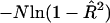, where N is the number of sib pairs in the sample and is the estimated proportion of variance explained by the regression (Mood et al. 1974, pp. 494–497). When is small, this becomes approximately . For large samples, the distribution of this statistic is χ²₁ with noncentrality parameter (NCP) approximately equal to NR². The necessary variances for calculation of the population R² for the three HE methods are derived in Appendix A, and the NCPs (per sib pair) for the three HE regressions are given in table 1.

Table 1.

NCPs for HE Regressions

Model	Dependent	Variance of Dependent	Variance Explained	NCP (per Sib Pair)
HE-SS	(X+Y)2	8(1+r)2
HE-SD	(X-Y)2	8(1-r)2
HE-CP	XY	1+r2

When the sib correlation r is 0, the NCPs for HE-SS and HE-SD are the same, and they sum to the NCP of HE-CP. With increasing r, HE-SD gains power whereas HE-SS and HE-CP lose power; when , the NCP of HE-CP falls below that of HE-SD.

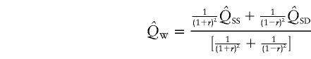
Xu et al. (2000) suggested a unified HE method that uses a linear combination of the estimates of Q from HE-SS and HE-SD, where the weights are given by the sample variances and covariance of the two estimates. However, since the covariance between squared sums and squared differences is 0 (Appendix A), the covariance between the estimates of Q from HE-SS and HE-SD, from large samples, is also 0, and the optimal weight for each estimate of Q is simply the inverse of its variance. We shall call this weighted method “HE-W.” The pooled estimate of Q, and its sampling variance (derived in Appendix B) for N sib pairs are given by

and

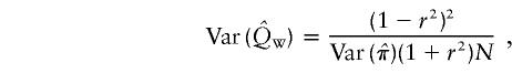where and are the separately estimated QTL variances from HE-SS and HE-SD regressions, respectively. The square of the pooled estimate divided by its variance provides a χ² test for linkage. The NCP (per sib pair) of this test is given by

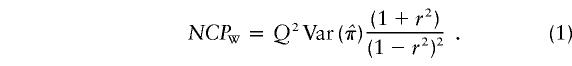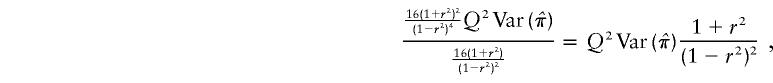
This is equal to the sum of the NCPs of HE-SS and HE-SD and is identical to the NCP of VC linkage analysis (Rijsdijk et al. 2001). The NCP for the linkage test in a VC model is given by the asymptotic expectation of the likelihood-ratio statistic:

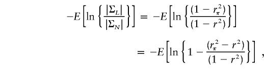where r_π is the sib correlation conditional of ; that is, 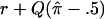. By taking Taylor’s expansion to the second order and simplifying, we obtain

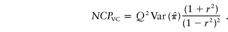This demonstrates equivalence, in asymptotic power, between the HE-W method and the standard VC model, for random samples of sib pairs. We can simplify the HE-W method further by noting that, instead of performing two separate regression analyses (HE-SS and HE-SD) and combining the estimates, we can obtain the same NCP by regressing a weighted sum of the squared sums and squared differences on , where the weights for the squared sums and squared differences are inversely proportional to their variances (See Appendix C):

We have confirmed the equivalence between this new combined HE regression (HE-COM) and VC linkage analysis, by simulation. Trait data for sib pairs were generated under a series of models where an additive QTL accounts for either 5% or 10% of the phenotypic variance and where the shared residual variance between sibs ranges from 0% to 50%. A completely informative marker is assumed, so that the sib pairs have values of 0, .5, and 1 in the proportions .25, .5, and .25, respectively. For each model, 500 replicates of 10,000 sib pairs were generated; each replicate was subjected to HE-SS, HE-SD, HE-CP, HE-W, HE-COM, standard VC, and the robust VC conditioning on trait values (VC-C) approach (Sham et al. 2000). The results show that the χ² statistics of HE-W, HE-COM, and VC analyses have almost identical means and variances and are almost perfectly correlated (for 5% QTL, see fig. 1; results for 10% QTL showed the same patterns). As predicted, the HE-SS, HE-SD, and HE-CP methods have smaller average χ² test statistics than do HE-W, HE-COM, or VC analysis. As sib correlation increases, the power of the original HE method (i.e., HE-SD) approaches that of the VC model.

Figure 1.

Unselected samples: mean χ² statistics from HE and VC methods, as a function of residual sib correlation. Each mean is based on 500 simulated replicates of 10,000 sib pairs. The QTL is additive and accounts for 5% of trait variance.

Although HE-W and HE-COM give equivalent χ² statistics in these simulations, we prefer HE-COM, since it will remain valid even when squared sums and squared differences are not orthogonal, as may be the case in samples selected for extreme trait values. The use of HE-COM requires knowledge of the trait mean and variance (in order to standardize the trait values) and of the correlation between sibs (in order to optimally weight the squared sums and squared differences). If, in addition, the weighted sum of squared sums and squared differences is mean adjusted according to the population sib correlation (by addition of 4r/(1-r²)), and, if the intercept of the regression fixed at 0, then the HE-COM method will also provide a robust and powerful test for linkage in any selected sample, analogous to VC-C (Sham et al. 2000). Indeed, the square of the mean-adjusted weighted sum of squared differences and squared sums is an index that is proportional to the expected sib-pair NCP conditional on trait values. This index can be used to rank order sib pairs in terms of their potential informativeness to facilitate selective genotyping. The resulting selection profile is virtually identical to our VC-based strategy for selective genotyping (Purcell et al. 2001). The index attenuated by a factor of Q²/16 gives the actual expected NCP (per sib pair) for complete IBD information:

Figure 2 plots the expected NCP as a function of sib-pair trait values, for the case of a sibling correlation of .25 and Q=.05.

Figure 2.

Surface plot of expected sibship NCP, as a function of trait scores, based on equation (3), for a QTL accounting for 5% of phenotypic variance and a sib correlation of .25.

To confirm that HE-COM provides a valid test of linkage in selected samples, we ran simulations in which, among a random sample of 10,000 pairs, only the most informative 5% of sib pairs (according to expected NCP) were analyzed. The trait mean, variance, and sibling correlation were fixed at the true population values. Comparing HE-COM, VC-C, and the standard VC approach under the null (i.e., no QTL effect was simulated), we found that HE-COM and VC-C gave expected χ² statistics around the appropriate level (i.e., .5). In contrast, standard VC analysis is liberal when applied to selected samples. This result is well known, and so standard VC analysis was not considered further, since it does not provide a valid test for selected data. For data simulated under a model with a QTL accounting for 5% of the trait variance, HE-COM gives average χ² values that are only slightly less than those of VC-C. This demonstrates the approximate equivalence of the two methods when applied to selected samples (fig. 3).

Figure 3.

Selected samples: mean χ² statistics from the HE-COM, standard VC, and VC-C, as a function of residual sib correlation. Each mean is based on 500 simulated replicates, with selection of the most informative 500 sib pairs from 10,000, simulating either a QTL accounting for 5% of the trait variance or no QTL effect (for which the expected χ² value is 0.5). Note that the standard VC is not included under the 5% QTL scenario, since it is liberal in selected samples, as can be seen when no QTL effect is simulated.

The power of HE-COM—and, indeed, that of all HE methods—can be improved by taking into account the degree to which locus-specific IBD sharing of a sib pair can be inferred from marker genotypes. The least-squares estimation procedure can be improved by giving less weight to sib pairs in which IBD sharing is ambiguous. The extension of HE-COM both to take account of incomplete IBD information and to multiple traits and general pedigrees may lead to an attractive method for the linkage analysis of quantitative traits.

Appendix A: Variances and Covariances

Let X and Y be bivariate normal sib trait values that have mean 0, variance 1, and sib correlation r. A QTL contributes additive variance Q. Using the result that the square of a standard normal variable has a χ²₁ distribution and therefore variance 2, we can show the variance of the squared sums and squared differences to be, respectively,

and

The variance of the cross-products XY is given by consideration of the identity

which implies Var(XY)=1+r².

Finally, since (X+Y) and (X-Y) are jointly normal (being linear combinations of normal variables) and uncorrelated, it follows that (X+Y)² and (X-Y)² are also uncorrelated.

Appendix B: NCP for HE-W

A weighted estimate of Q from HE-SS and HE-SD is

with variance

The NCP (per sib pair) of this test is therefore as given in equation (1).

Appendix C: HE-COM Regression Equation

and

The regression equation is therefore equation (2). The NCP (per sib pair) is

which, again, is equivalent to that given by equation (1).

References

- Drigalenko E (1998) How sib-pairs reveal linkage. Am J Hum Genet 63:1242–1245 [PMC free article] [PubMed] [Google Scholar]
- Elston RC, Buxbaum S, Jacobs KB, Olson JM (2000) Haseman and Elston revisited. Genet Epidemiol 19:1–17 [DOI] [PubMed] [Google Scholar]
- Haseman JK, Elston RC (1972) The investigation of linkage between a quantitative trait and a marker locus. Behav Genet 2:3–19 [DOI] [PubMed] [Google Scholar]
- Mood AM, Graybill FA, Boes DC (1974) Introduction to the theory of statistics. MaGraw-Hill International, Singapore [Google Scholar]
- Purcell S, Cherny SS, Hewitt JK, Sham PC (2001) Optimal sibship selection for genotying in quantitative trait locus linkage analysis. Hum Hered 52:1–13 [DOI] [PubMed] [Google Scholar]
- Rijsdijk FV, Hewitt JK, Sham PC (2001) Analytic power calculation for variance-components linkage analysis in small pedigrees. Eur J Hum Genet 9:335–340 [DOI] [PubMed] [Google Scholar]
- Sham PC, Zhao JH, Cherny SS, Hewitt JK (2000) Variance-components QTL linkage analysis of selected and non-normal samples: conditioning on trait values. Genet Epidemiol 10 Suppl 1:S22–S28 [DOI] [PubMed] [Google Scholar]
- Wright F (1997) The phenotypic difference discards sib-pair QTL linkage information. Am J Hum Genet 60:740–742 [PMC free article] [PubMed] [Google Scholar]
- Xu X, Weiss S, Xu X, Wei LJ (2000) A unified Haseman-Elston method for testing linkage with quantitative traits. Am J Hum Genet 67:1025–1028 [DOI] [PMC free article] [PubMed] [Google Scholar]