Aphasia Severity Prediction Using a Multi-modal Machine Learning Approach

Abstract

The present study examined an integrated multiple neuroimaging modality (T1 structural, Diffusion Tensor Imaging (DTI), and resting-state FMRI (rsFMRI)) to predict aphasia severity using Western Aphasia Battery-Revised Aphasia Quotient (WAB-R AQ) in 76 individuals with post-stroke aphasia. We employed Support Vector Regression (SVR) and Random Forest (RF) models with supervised feature selection and a stacked feature prediction approach. The SVR model outperformed RF, achieving an average root mean square error (RMSE) of 16.38 ± 5.57, Pearson’s correlation coefficient (r) of 0.70 ± 0.13, and mean absolute error (MAE) of 12.67±3.27, compared to RF’s RMSE of 18.41±4.34, r of 0.66±0.15, and MAE of 14.64±3.04. Resting-state neural activity and structural integrity emerged as crucial predictors of aphasia severity, appearing in the top 20% of predictor combinations for both SVR and RF. Finally, the feature selection method revealed that functional connectivity in both hemispheres and between homologous language areas is critical for predicting language outcomes in patients with aphasia. The statistically significant difference in performance between the model using only single modality and the optimal multi-modal SVR/RF model (which included both resting-state connectivity and structural information) underscores that aphasia severity is influenced by factors beyond lesion location and volume. These findings suggest that integrating multiple neuroimaging modalities enhances the prediction of language outcomes in aphasia beyond lesion characteristics alone, offering insights that could inform personalized rehabilitation strategies.

1. Introduction

Aphasia has been recognized as the condition most adversely affecting quality of life, surpassing even cancer and Alzheimer’s disease (Lam and Wodchis, 2010). It is commonly associated with ischemic stroke, with 30% of ischemic stroke patients experiencing aphasia. This ratio has remained stable over the past 20 years, despite an increasing aging population and decreasing stroke mortality (Grönberg et al., 2022; Li et al., 2020; Modig et al., 2019). Given its significant negative impact on patients’ quality of life, predicting aphasia severity to provide an accurate prognosis is crucial for patients to receive effective treatment.

Past research has indicated that lesion size and location are key predictors of aphasia severity (Forkel et al., 2014; Fridriksson et al., 2016; Hope et al., 2013, 2018; Ramsey et al., 2017; Wang et al., 2013; Yourganov et al., 2015). Nevertheless, the location of the lesion alone may not provide the complete picture. Geller et al. (2019) found that compared to lesion load, white matter tract disconnection is a stronger predictor of individual deficits, such as speech production. Additionally, functional connectomes measured by resting-state functional connectivity correlate with behavioral measures of speech and language (Yourganov et al., 2018). Previous literature has shown that different neuroimaging modalities provide complementary information, enhancing the understanding of aphasia’s neural substrates (Billot et al., 2022; Chennuri et al., 2023; Crosson et al., 2019; Gaizo et al., 2017; Halai et al., 2020; Kristinsson et al., 2020; Kuceyeski et al., 2016; Pustina et al., 2017; Yourganov et al., 2016). Given their flexibility and capability to capture intricate data patterns, machine learning methods are frequently employed to analyze complex patterns in multimodal data (Billot et al., 2022; Gaizo et al., 2017; Halai et al., 2020; Kertesz, 2012; Kristinsson et al., 2020; Pustina et al., 2017; Yourganov et al., 2016).

For example, Yourganov et al. (2016) utilized a linear kernel Support Vector Regression (SVR) model (Awad and Khanna, 2015) to predict speech and language abilities in individuals with post-stroke aphasia. They integrated lesion-load data from structural MRI and connectome data, measuring the number of Diffusion Tensor Imaging (DTI) tracts connecting each pair of gray matter regions (Yourganov et al., 2016). Although their prediction for the Western Aphasia Battery-Revised Aphasia Quotient (WAB-R AQ) (Kertesz, 2012) using combined connectome and lesion data (r = 0.69) was similar to using lesion data alone (r = 0.69), the connectome provided additional spatial information. Another study found that using linear SVR to combine connectome data derived from DTI and lesion-load maps improved WAB-R AQ score prediction (r = 0.76) compared to using lesion-load maps alone (r = 0.72) (Gaizo et al., 2017). Halai et al. (2020) systematically analyzed the influence of brain partition methods, combinations of different neuroimaging measures derived from Diffusion-Weighted Imaging (DWI) and structural MRI, and types of machine learning models on aphasia severity prediction. They concluded that adding DWI data to lesion-load models did not significantly improve model accuracy, and different brain partition methods did not produce significantly different results.

Beyond examining structural measures like DTI and structural MRI, some studies have incorporated functional MRI into their analysis. Kristinsson et al. (2020) applied a radial kernel SVR model (Awad and Khanna, 2015) to predict WAB-R AQ using task activation maps acquired from task-based functional MRI (fMRI), fractional anisotropy (FA) values derived through DTI, cerebral blood flow, and lesion-load maps. They found that the improvement in accuracy of the multi-modal model predictions was statistically significant (p < 0.05) compared to any single modality model. Another multi-modal study leveraged lesion-load maps, structural connectivity measures from DTI, and functional connectivity measures from resting-state fMRI using Random Forest (RF) models to estimate aphasia severity (Pustina et al., 2017). For WAB-R AQ prediction, the best single modality measure was the resting-state connectivity matrix (r = 0.81), and the multimodal prediction was systematically more accurate (r = 0.88, p < 0.001). Resting-state fMRI data has also emerged to be an an important predictor for patients’s responsiveness to aphasia treatment. Specifically, our previous work examined multimodal neuroimaging and demographic data to predict patients’ responsiveness to aphasia treatment (Billot et al., 2022). We found that models integrating a subset of multimodal data (accuracy = 0.927, F1 = 0.941, precision = 0.914, and recall = 0.970) outperformed those trained on any single modality. Furthermore, resting-state functional connectivity was an important predictor both alone and in combination with other modalities.

In general, the studies discussed above are challenged by the issue of a large number of predictors relative to small sample sizes, which increases the risk of over-fitting in the development of predictive models using multi-modal neuroimaging data. To mitigate this problem, researchers have used data reduction strategies, such as preselecting relevant variables. For instance, Kristinsson et al. (2020) applied univariate regression for feature selection, while Pustina et al. (2017) utilized the recursive feature elimination (RFE) procedure. However, many studies use statistically significant correlations as an indicator of predictive power (Basilakos et al., 2014; Chennuri et al., 2023; Yourganov et al., 2016), which can lead to poor predictive models because these variables are not always the best predictors (Lo et al., 2015). To address this issue, the present research utilizes a supervised learning scheme with Recursive Feature Elimination (RFE) (Guyon et al., 2002) to select more informative and robust features (Pustina et al., 2017). Additionally, previous work has often pre-selected features from the entire dataset (Kristinsson et al., 2020; Pustina et al., 2017) before the training and testing split, which can introduce the risk of data leakage. To avoid this, we use a nested cross-validation procedure and only selected features within each training set using the supervised learning scheme.

Even though recent work has identified the importance of multimodal models, caveats in the feature selection process have led to suboptimal predictive models. This paper aims to provide systematic comparisons in predicting aphasia severity, as indicated by WAB-R AQ, using two common types of machine learning model across multiple modalities. Specifically, we will deploy robust and informative feature selection methods to enhance model performance; evaluate and compare the performance of RF and SVR models, as well as models utilizing single-modality and combined modalities. Furthermore, building on prior work highlighting the importance of rsFMRI connectivity in predicting patients’ responsiveness to treatment (Billot et al., 2022), we evaluate the extent to which rsFMRI connectivity predicts aphasia severity in this work.

2. Materials and Methods

Figure 1 presents the methodological framework of the study. A total of 76 individuals from two cohorts with left hemisphere stroke were included in the study (See Table 1 for overview of demographic information of two cohorts). Figure 2 shows the lesion overlay for all participants, revealing a broad distribution of damage across the language network. The ten most frequently lesioned ROIs—insula, Rolandic operculum, Heschl’s gyrus, superior temporal gyrus, putamen, pars opercularis, supramarginal gyrus, pars triangularis, middle temporal gyrus, and superior temporal pole—span multiple lobes and the MCA territory.

Figure 1:

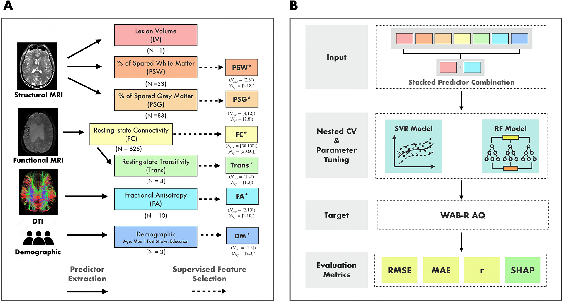
Methodological Framework of the Study. A. Demographic and neuroimaging data were collected for all participants. Neuroimaging data were preprocessed, and predictors were extracted from different modalities. Colored boxes indicate the predictors derived from different modalities. The total number of features in each predictor before passing to the feature selection is presented below each box. Boxes marked with an asterisk (*) indicate a subset of features from the original predictors, selected through a supervised feature selection method. For these predictors, the range of features retained after selection across “outer” cross-validation folds is shown below each box. LV: Lesion Volume, PSW: Percent of Spared White Matter, PSG: Percent of Spared Grey Matter, FC: Resting-State Functional Connectivity Matrix, Trans: Transitivity Score, FA: Fractional Anisotropy, and DM: Demographic. B. All combinations (N = 127) of predictors were tested as inputs to the Support Vector Regression (SVR) and Random Forest (RF) models to predict participants’ WAB-R AQ. For each predictor combination, the features from the selected predictors were stacked together to form a single, extended input feature set. Model performance was evaluated using Root-mean-squared-error (RMSE) as the primary metric along with mean-absolute-error (MAE) and correlation (r). Furthermore, Shapley values (SHAP) with RMSE as the characteristic function, are calculated for each predictor.

Table 1:

Overview of Demographic Information of Two Cohorts

	Cohort 1 (N = 30)	Cohort 2 (N = 46)	Overall (N = 76)
Age (mean years) (±Std)	58.50 (11.61)	59.52 (10.68)	59.12 (10.99)
Month Post Stroke (mean months) (±Std)	84.40 (100.40)	51.72 (39.82)	64.61 (71.47)
Education Years (mean years) (±Std)	15.87 (2.83)	16.03 (2.06)	15.97 (2.37)
WAB-R AQ (mean) (±Std)	76.85 (23.69)	69.14 (23.28)	72.16 (23.57)

Figure 2:

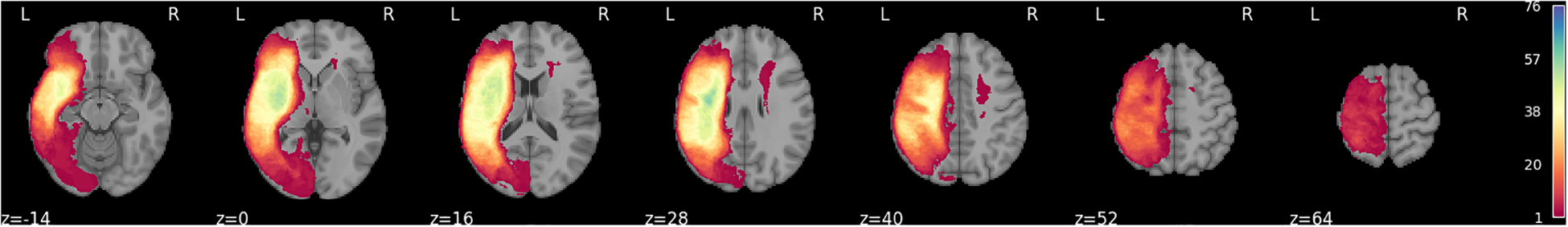
Lesion overlay for the 76 participants in the study.

In terms of clinical profiles, our sample includes a range of aphasia subtypes: 41 anomic, 21 Broca’s, 7 conduction, 3 Wernicke’s, 2 transcortical motor, 1 transcortical sensory, and 1 global aphasia. This distribution reflects a heterogeneous sample with diverse lesion patterns and symptom presentations.

Neuroimaging data—structural MRI, resting-state fMRI, and DTI—and demographic information were collected for all individuals. The data used for this analysis are in the process of being uploaded to Open Science Framework (OSF) and will be available at the following link: http://osf.io/mcu36. In the interim, data are available from the authors upon request. All participants provided written informed consent before study participation. The study protocol for Cohort 1 was approved by the institutional review boards at Boston University. Participants included in Cohort 2 were recruited from Boston University (N = 24), Johns Hopkins University (N = 15), and Northwestern University (N = 7). The study protocol for Cohort 2 was approved by the institutional review boards at Boston University, Massachusetts General Hospital, Northwestern University, and Johns Hopkins University.

2.1. Cohort 1

2.1.1. Participants

Participants were 30 individuals with chronic post-stroke aphasia (26 male, 4 female) due to a single left-hemisphere stroke. They were recruited as part of a broader project (Grant NIDCD R01DC016950) evaluating the role of a domain-general multiple-demand network in functional reorganization supporting recovery in post-stroke aphasia. All participants were fluent English speakers, had normal or corrected-to-normal hearing and vision, were medically and neurologically stable, between the ages of 35 and 80 years, and had received at least a high school education. Participants were excluded if they were ineligible for MRI, had comorbid neurological conditions, were unable to perform tasks in the MRI, or incomplete/missing neuroimaging data.

2.1.2. MRI Acquisition & Preprocessing

MRI parameters.

Images were acquired using Siemens 3.0T Prisma scanners. Structural images were acquired for all participants using the T1 MEMPRAGE (176 sagittal slices, 1 mm × 1 mm × 1 mm voxel size, TR = 2530 ms, TE₁ = 1.69 ms, TI = 1100 ms, flip angle = 7°) sequence. When possible, additional structural images were acquired using T2-SPACE FLAIR (176 sagittal slices, 1 mm × 1 mm × 1 mm voxel size, TR = 6000 ms, TE = 456 ms, TI = 2100 ms). A high-resolution whole-brain DTI sequence was also completed (TR = 3100 ms, TE = 80.80 ms, flip angle = 78°, FOV = 208 × 208 mm², voxel size = 2.0 × 2.0 × 2.0 mm³, 78 interleaved slices with 102 gradient directions and 10 non-diffusion weighted (b = 0) volumes, b value = 3000 s/mm²). Functional scans were acquired using an SMS EPI sequence (81 slices, 2.4 mm × 2.4 mm × 1.8 mm voxel size, TR = 2000 ms, TE = 32 ms, flip angle = 80°, A≫P phase encoding direction, 216 mm FoV, interleaved multi-slice mode). During the resting state scan, participants were instructed to allow their minds to wander and to stay awake.

Lesion mapping.

Stroke lesion maps were generated using the semi-automated segmentation tool ITK-SNAP (Yushkevich et al., 2006). This approach uses Random Forest classification mode, using samples of lesioned and non-lesioned tissue manually selected based on the scans. Using information (i.e., voxel intensity, neighboring voxel intensity, and voxel coordinates) from available structural images, a seed image is generated in which each voxel is assigned a probability of belonging to the lesion. Active contour evolution originating from an operator-defined seed location within the lesion generates the final lesion segmentation (i.e., a binary map where lesioned voxels have a value of 1 and non-lesioned voxels have a value of 0) (Yushkevich et al., 2006). The accuracy of each stroke lesion map was visually inspected and, if necessary, the process was repeated using additional samples to optimize performance.

Diffusion-weighted imaging.

To address any distortions or movement observed during scanning, the TOP UP and Eddy functions of the FMRIB Software Library (FSL) version 6.0.4 were utilized. Corrections were made to the identified distortions, and then the refined images were transferred to DSI Studio for further tractography and analysis. Within DSI Studio, image reconstruction was performed using Generalized Q-sampling Imaging (GQI) aligned with the ICBM152 adult template. No alterations were made to the white matter coverage in the reconstruction masks to maintain the precision of the analysis in DSI Studio and to prevent the inadvertent exclusion of white matter areas. Additionally, preprocessing the images outside of DSI studio improved the quality of the input images, so filtering distortions was not a concern. The default parameters were applied, which included a diffusion sampling length ratio of 1.25. Additionally, the b-table was manually audited to check the quality of the corrected scans. Atlas-based tractography was then conducted, again using the ICBM152 adult atlas. The default tracking parameters were applied to the tracking, which included a tracking index of 99, tracking threshold of 0, angular threshold of 0, step size of 0, minimum length of 30 mm, and maximum length of 200 mm. Typology informed pruning was conducted in DSI studio as well, and the default threshold of 4 and autotrack tolerance of 24 mm were applied. No additional thresholds or filters were applied. In total 10 tracts of interest were investigated. These include the bilateral arcuate fasciculus (AF), superior longitudinal fasciculus I (SLF), inferior longitudinal fasciculus (ILF), inferior fronto-occipital fasciculus (IFOF), and uncinate fasciculus (UF). Following tract reconstruction, fractional anisotropy (FA) metrics were extracted. FA values, which range from 0 to 1, indicate the directionality of water molecule diffusion within white matter tracts. Values closer to 1 suggest more restricted and directionally oriented diffusion, indicative of higher tract integrity.

Resting-state fMRI.

Functional and anatomical data were preprocessed using a flexible preprocessing pipeline (Nieto-Castanon, 2020) including realignment, outlier detection, direct MNI-space normalization, masking, regression of temporal components, band-pass filtering, and masked smoothing. Anatomical data were normalized to standard MNI space, segmented into gray matter, white matter, CSF, and lesion tissue classes, and resampled to 1 mm isotropic voxels using the SPM unified segmentation and normalization algorithm (Ashburner and Friston, 2005; Ashburner, 2007) with an alternative tissue probability map (TPM) template extended to include custom lesion masks. Functional data were coregistered to a reference image (first scan of the first session) using a least squares approach and a 6 parameter (rigid body) transformation (Friston et al., 1995), and resampled using b-spline interpolation. Potential outlier scans were identified using artifact detection tools (ART) (Whitfield-Gabrieli et al., 2011) as acquisitions with framewise displacement above 0.9 mm or global BOLD signal changes above 5 standard deviations (Power et al., 2014; Nieto-Castanon, 2022), and a reference BOLD image was computed for each subject by averaging all scans excluding outliers. Functional data were normalized into standard MNI space and resampled to 2 mm isotropic voxels following a direct normalization procedure using SPM unified segmentation and normalization algorithm (Ashburner and Friston, 2005; Ashburner, 2007) with an alternative tissue probability map (TPM) template. Functional images were masked setting all voxels within a custom mask area to zero. Components from realignment, and scrubbing were removed from the BOLD signal timeseries using a separate linear regression model at each individual voxel. BOLD signal timeseries were bandpass filtered between 0.01 Hz and 0.25 Hz. Last, functional data were smoothed using spatial convolution with a Gaussian kernel of 4 mm full width half maximum (FWHM) while disregarding all voxels outside a custom mask area.

2.2. Cohort 2

2.2.1. Participants

Participants were 46 chronic PWA (30 male, 16 female) due to a single left-hemisphere stroke. Participants were selected from a larger sample (N = 76) who had completed a multi-site study between 2015 and 2018 examining neurobiological features of aphasia recovery (NIDCD P50DC012283). All participants met the following inclusion criteria: chronic aphasia due to a single left-hemisphere stroke, monolingual English-speaking, medically and neurologically stable, normal or corrected-to-normal hearing and vision, at least a high school education, between the ages of 35 and 80, and at least one year post-stroke. Participants were excluded if they were ineligible for MRI, had comorbid neurological conditions, were unable to perform tasks in the MRI, or had incomplete or missing neuroimaging data. Behavioral and neuroimaging findings associated with this cohort of participants have been reported in previous publications (Billot et al., 2022; Braun et al., 2022; Falconer et al., 2024; Gilmore et al., 2020; Johnson et al., 2019, 2020, 2021; Meier et al., 2019a,b).

2.2.2. MRI Acquisition & Preprocessing

MRI parameters.

T1-weighted sagittal imaging was collected (TR/TE = 2300/2.98 ms, TI = 900 ms, flip angle = 9°, voxel size = 1 × 1 × 1 mm³, 176 sagittal slices with a slice thickness of 1 mm). A high-resolution whole-brain cardiac-gated DTI sequence was also completed (TR_eff > 7.5 sec depending on the HR, TE = 92 ms, flip angle = 90°, FOV = 230×230 mm², voxel size = 1.983×1.983 2.000 mm³, 72 interleaved slices with 60 gradient directions and 10 non-diffusion weighted (b = 0) volumes, b value = 1500 s/mm²). There were slight variations in TE values for both structural sequences based on the different scanners at Johns Hopkins University and Northwestern University (for T1, TE = 2.91 − 2.95; for DTI, TE = 64 − 92) to ensure the same quality of data. At Johns Hopkins University, voxel size of the DTI images was 1.797 × 1.797 × 2.000 mm³ and one non-diffusion weighted (b = 0) volume was acquired. Whole-brain functional images were collected using a gradient-echo T2*-weighted sequence (TR =2000 or 2400 sec, TE = 20 ms, flip angle = 90°, voxel size = 1.72 × 1.72 × 3 mm³, 210 or 175 interleaved slices).

Lesion mapping.

Lesion tracing was done manually in MRIcron by trained research assistants based on the 3D T1-weighted images, which were viewed simultaneously in three orthogonal planes to ensure precise identification. For this cohort, the manual tracing was completed before the ITKSNAP implementation pipeline was validated in our group.

Diffusion-weighted imaging.

FA values in this cohort were calculated using a different preprocessing pipeline than the Cohort 1. Briefly, preprocessing steps for diffusion-weighted imaging included 1) denoising using principal components and creation of a b0 reference image from the mean of the non-diffusion-weighted scans, 2) skull stripping of the T1 structural image, rigidly aligning a pseudo-T2 image to the b0, 3) nonlinear distortion correction, 4) eddy current correction and creating rotated b-vectors, 5) concatenation of eddy current corrected parameters with the b0 distortion field that was then applied to the diffusion scans, and 7) calculation of the diffusion tensor using the nonlinear weighted positive definite tensor-fitting algorithm from Camino (Cook et al., 2006).

Post-processing of diffusion tensor imaging data was then completed using Automated Fiber Quantification (AFQ), which completes deterministic tractography using MATLAB. The tractography algorithm provided fractional anisotropy (FA) values for 100 nodes along each delineated tract for the same 10 tracts of interest analyzed in the section: AF, UF, IFOF, ILF, and SLF. FA values were then averaged across each tract to yield one FA value per delineated tract per participant (up to 10 FA values per participant). In the left-hemisphere, tracts with missing values were replaced with 0 given the higher likelihood of missing data secondary to damaged white matter; in the undamaged right-hemisphere, missing values were replaced with the mean of all participants’ values for that tract (Braun et al., 2022). The FA values calculated using this approach for Cohort 2 were not statistically different from those of the Cohort 1 except for right SLF (see Supplementary Figure S1).

Resting-state fMRI.

The same steps for preprocessing the anatomical and functional data as Cohort 1 were applied to Cohort 2.

2.3. Modality Predictors

From three imaging modalities—structural MRI, functional MRI, and DTI—six predictors were calculated. Using structural MRI, we calculated three predictors: lesion volume (LV), the percentage of spared grey tissue (PSG), and the percentage of spared white tissue (PSW). PSG was computed for 83 left hemisphere gray matter regions of the Automated Anatomical Labeling Atlas 3 (AAL3) (Rolls et al., 2020). This was done by resampling lesion masks to match the dimensions of the AAL3 atlas and then calculating the proportion of non-overlapping voxels between each lesion and each of the 83 left hemisphere AAL3 regions. PSW was calculated for 36 white matter tracts using the Tractotron feature in BCBToolkit (Foulon et al., 2018). In this module, lesions from each patient were mapped onto tractography reconstructions of white matter pathways obtained from a group of healthy controls (Rojkova et al., 2016). The percentage of spared white matter was calculated by subtracting the proportion of overlap between the lesion mask and each tract’s volume from 1. Right hemisphere regions were excluded from analysis, as all patients had left hemisphere strokes. Although most of the white matter tracts provided by BCBToolkit were bilateral, four tracts that span both hemispheres (anterior commissure, frontal commissure, corpus callosum, and fornix) were included in the analysis, bringing the total to 36 tracts.

From the rsfMRI data, ROI-to-ROI connectivity matrices were used to characterize the resting-state functional connectivity between 50 pre-selected ROIs (see Supplementary Table S1) of the AAL3 atlas (Rolls et al., 2020). The method for selecting these ROIs follows the approach detailed in (Falconer et al., 2024). ROIs were selected based on consistent support from prior literature regarding their roles in relevant neurocognitive domains and their inclusion in functional networks identifiable at rest. For the language network, ROIs encompassed regions associated with naming, semantic processing, written word production, and sentence comprehension. Similarly, ROIs for the default mode, dorsal attention, and salience networks were defined based on meta-analyses showing their consistent involvement in these networks. Then, ROI-to-ROI connectivity strength was represented by Fisher-transformed bivariate correlation coefficients of ROIs’ BOLD signal time series. These matrices were reduced to 625 values (rsFMRI-FC) by excluding non-homologous interhemispheric connections (Billot et al., 2022). After computing the 50 × 50 ROI-to-ROI connectivity matrix, we extracted submatrices corresponding to brain regions within the Language Network, Dorsal Attention Network, Salience Network, and Default Mode Network. Transitivity scores (rsFMRI-trans), a measure of the clustering coefficient, were calculated as the ratio of triangles to triplets in the network for these four networks using the Brain Connectivity Toolbox (Rubinov et al., 2009).

From DTI, FA values were extracted from 10 tracts including the bilateral arcuate fasciculus, superior longitudinal fasciculus I, inferior longitudinal fasciculus, inferior fronto-occipital fasciculus, and uncinate fasciculus using methods decribed in the paragraph 2.1.2 and 2.2.2.

Normalized Features.

Furthermore, all features in the predictors except demographic range between 0 and 1. Demographic information is normalized between 0 and 1 with min-max normalization (Demircioğlu, 2024).

2.4. Model Development

We tested two types of machine learning models: RF (Breiman, 2001) and SVR (Awad and Khanna, 2015). For the SVR model, we tested both linear and Radial Basis Function (RBF) kernels (Awad and Khanna, 2015). Models were trained, tuned, and tested using a nested Cross-Validation (CV) scheme, illustrated in Fig. 3, consisting of an “outer” random partitioning of the complete dataset into 11 test-training folds for performance evaluation, with each training fold further randomly partitioned, ten times, into 10 validation-training folds for feature selection, model training and hyperparameter tuning. Pseudocode for feature selection, model training and tuning is provided in Supplementary Algorithm 1 and explained below in detail.

Figure 3:

Graphic Illustration of Model Development. The complete dataset is first split randomly into 11 test-training folds. Each “outer” training fold is further divided randomly, ten times, into 10 “inner” Cross-Validation (CV) folds for a total of 100 inner validation-training folds. For each k, Recursive Feature Elimination (RFE) is applied to each of the 100 inner training folds to select the k most important features. The top k most frequently selected features across all 100 inner training folds is then used to train a machine learning (ML) model and tune its hyper-parameters using the same 100 inner validation-training folds. The trained and tuned model with the lowest average validation RMSE across all k values is used to predict the WAB-R AQ of the outer test fold. The final test performance is the average value of the test metric across all 11 outer test folds.

Supervised Feature Selection.

To address the imbalance between the large number of features in certain predictors, namely PSW, PSG, and rsFMRI-FC, and the limited sample size, feature selection was necessary. To ensure the feature selection process remained independent of the testing data, each of the 11 outer training folds was randomly split, ten times, into 10 inner validation-training folds. These 100 inner validation-training folds were used for feature selection, training, and model hyperparameter tuning.

Recursive Feature Elimination (RFE).

To determine the optimal number and subset of features for each predictor (except LV which has only one feature), we utilized RFE (Guyon et al., 2002), a supervised feature selection method that recursively reduces the feature set size. For each model type—SVR or RF—the model is initially trained on the complete set of features within the predictor, generating an importance score for each feature. In RF, this score is based on how much each feature reduces impurity across splits, while in SVR with a linear kernel, it is based on the absolute value of each feature’s coefficient, reflecting its contribution to predictions (note that all features are normalized to the range [0, 1]). At each step, RFE removes the bottom 40% of features with the lowest importance scores, repeating the process until only the specified number k of features remains. For SVR, feature selection was performed only using the linear kernel, with feature importance scores derived from model coefficients which directly indicate each feature’s contribution. Since the RBF kernel SVR lacks individual feature coefficients, feature importance cannot be determined similarly. Instead, we used the features selected using the linear kernel to train and tune the RBF kernel SVR to capture non-linear relationships. For each k, RFE was applied to each of the 100 inner training folds to select, for each fold, the k features with the highest importance scores. For a given number k, we then counted the number of times (out of 100) each feature was selected by RFE across the 100 folds.

Model Training and Tuning and Best Models.

The top k most frequently selected features were used to train and tune the final model using the same 100 validation-training folds. This process was repeated for various values of k, and the best model for a given predictor and associated set of features was chosen as those with the best average RMSE validation performance across all values of k.² We note that since feature selection was independent of the test set, the optimal k and selected features could vary across outer folds. Additionally, because feature importance depends on the model type, the selected features could differ between model types.

Models for Predictor Combinations.

The reduced subset of features for each predictor was later used in the training, tuning, and testing of various combined-predictor models. Specifically, the selected subsets of features from different predictors were stacked together as inputs for the combined-predictor models, meaning that feature selection was only applied to each individual predictor before stacking, and no further feature selection was performed after the predictors were combined. Prediction models were created for all possible predictor combinations, resulting in 127 models (6 single-predictor and 121 combined-predictor) for each model type. The same inner repeated 10-fold cross-validation was used to train and tune the 121 combined-predictor models based on RMSE, with performance tested in the same outer cross-validation test folds. All experiments were conducted using the Scikit-learn library (Pedregosa et al., 2011).

2.5. Performance Evaluation and Comparison

Although feature selection for each predictor and model training and tuning were done using RMSE, each model’s test performance was evaluated using RMSE, Mean Absolute Error (MAE), and the correlation between ground truth and prediction (r). RMSE was the primary model development and evaluation metric due to its convenience, widespread use, and because assessments based on RMSE are more conservative compared to MAE (Chai and Draxler, 2014). The RMSE was computed for each outer fold, predictor combination, and model type. Two-tailed Wilcoxon signed-rank tests were then conducted to compare the performance of different predictor combinations using SciPy (Virtanen et al., 2020) in Python 3.8.10. We compared SVR/RF models trained on a single predictor with: the optimal SVR/RF model, which had the lowest average test RMSE. Statistical significance was assessed at α = 0.05.

To further assess the importance of each predictor for prediction accuracy, we employed SHAP (SHapley Additive exPlanations) values (Friedman, 1986), a concept from cooperative game theory. SHAP values for each predictor were calculated for SVR and RF model families separately based on how much, on average, each predictor contributes to increasing or decreasing the prediction accuracy, as measured by average RMSE across folds, when included with other predictors. Specifically, the SHAP value for each predictor, i, is computed using the following formula:

$$\begin{gathered} {\varphi }_i\left(F,v\right)=\frac{1}{\left|F\right|!}\sum _{S\subseteq F\backslash \left\{i\right\}}\left|S\right|!\left(\left|F\right|-\left|S\right|-1\right)!\left[v\left(S\right)-v\left(S\cup \left\{i\right\}\right)\right], \\ =\frac{1}{\left|F\right|}\sum _{L=0}^{\left|F\right|-1}\frac{1}{\left(\underset{L}{\left|F\right|-1}\right)}\sum _{\underset{\left|S\right|=L}{S\subseteq F\backslash \left\{i\right\}}}\left[v\left(S\right)-v\left(S\cup \left\{i\right\}\right)\right], \end{gathered}$$ (1)

where ϕ_i is the SHAP function, F is the set of all predictors (7 in total), S is any subset of F that does not include predictor i, ν(S) is the so-called characteristic function given by the average RMSE score for the model using the subset of predictors S, and $\left[v\left(S\right)-v\left(S\cup \left\{i\right\}\right)\right]$ is the marginal contribution of predictor i to the subset S. We note that a positive value of $\left[v\left(S\right)-v\left(S\cup \left\{i\right\}\right)\right]$ would imply that RMSE decreases (prediction accuracy improves) when predictor i is used in conjunction with the predictors in S than otherwise. For $S=\left\{\right\}$, the empty set, the best RMSE predictor for any outer test-training fold is the constant predictor equal to the mean value of the outer training fold. SHAP values were computed for each predictor using a customized Python script (https://github.com/xinyihu3721/MultimodalAphasiaPred).

3. Results

Figure 4a illustrates the overall squared error distributions for test samples across all predictor combinations for both SVR and RF models, with each distribution constructed from a total of 9,652 points (76 subjects × 127 predictor combinations). Figure 4b breaks down the squared error distributions by modality, with RF models represented in red and SVR models in orange, enabling a comparison across specific predictor types. Each distribution in this plot is generated from 76 samples. Both Figure 4a and 4b were created using the Kernel Density Estimation method with Python’s seaborn.kdeplot. Smoothing bandwidth adjustments (bw_adjust) of 0.2 were applied for Figure 4a, while a bandwidth adjustment of 0.6 was used for Figure 4b. These adjustments were chosen to optimize the visualization of the distributions in each figure.

Figure 4:

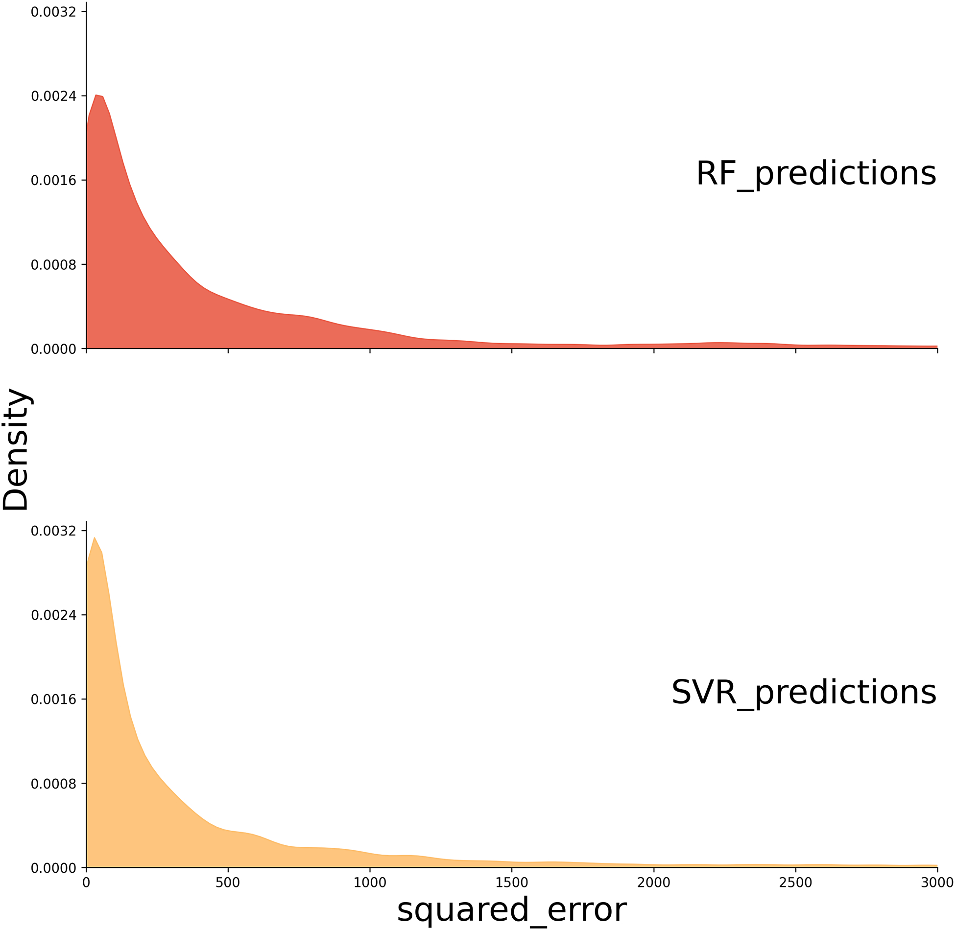
Squared Error Distribution Plots. (A) The distribution of squared errors for SVR and RF models. The plot indicates that SVR has a higher density of lower squared error values compared to RF. (B) The squared error distribution for each modality, with RF models represented in red and SVR models in orange. rsFMRI-FC: Resting State Functional Connectivity; rsFMRI-trans: Resting State Transitivity; PSG: Percent Spared Grey Matter; PSW: Percent Spared White Matter; LV: Lesion Volume; FA: Fractional Anisotropy; DM: Demographic; SVR: Support Vector Regression; RF: Random Forest.

In general, SVR shows a higher density of low squared error predictions (Figure 4), and significantly lower RMSE, as confirmed by a pairwise Wilcoxon test across all predictor combinations (p < 0.001) compared to RF (Figure 5). Because the SVR models consistently outperformed the RF models across all evaluation metrics, we focus our interpretation and discussion on the SVR results in the main text. Detailed outcomes from the RF models, including selected features and performance metrics, are provided in the Supplementary for reference. Additionally, no significant difference is observed between linear kernel and RBF kernel individual predictor SVR models (Supplementary Table S2). However, the RBF kernel, which can capture any non-linear relationships between rsFMRI-FC and PSW/PSG, has lower RMSE values for models that combine these predictors (Figure 6 model indices beyond 71). The remainder of this paper reports results for the optimal kernel for each predictor combination.

Figure 5:

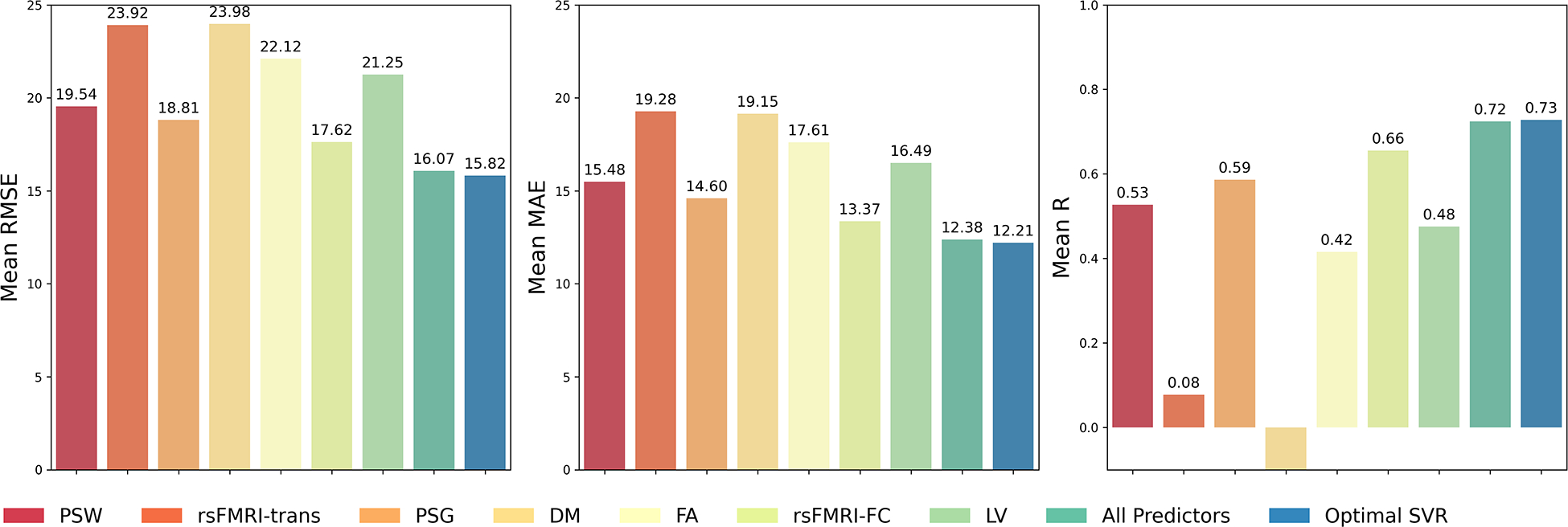
Predictive performance for Support Vector Regression (SVR) and Random Forest (RF) models trained on a single predictor, all predictors, or the optimal combination of predictors. The first column shows the average RMSE across the outer 11-fold cross-validation for all aforementioned types of predictors. The second column shows the average MAE, and the last column shows the mean r score. RMSE: Root Mean Squared Error; MAE: Mean Absolute Error

Figure 6:

Comparison of RBF Kernel and Linear Kernel Performance. This plot compares the average minimum RMSE achieved by each kernel type across different combined predictor models. The horizontal axis represents the index of the combined predictor model, and the vertical axis represents the RMSE value. The RBF kernel consistently achieved lower RMSE for models that combined rsFMRI-FC with PSW/PSG predictors (rsFMRI-FC: Resting State Functional Connectivity; PSG: Percent Spared Grey Matter; PSW: Percent Spared White Matter; RBF: Radial Basis Function).

3.1. SVR model predictions

When examining individual predictors, rsFMRI-FC alone has the lowest RMSE among single predictor SVR models. Additionally, single predictor models for PSG and PSW, which encode lesion location and structural integrity information of the brain, show the next lowest RMSE performances. The differences between rsFMRI-FC and PSG models are not statistically different (p > 0.05). DM, and rsFMRI-trans are not informative single predictors for SVR models (Figure 5).

Notably, the best SVR model was not the full-predictor model (Table 2). After ranking the SVR models with various predictor combinations, the SVR model with the lowest RMSE incorporated a combination of DM, PSW, and rsFMRI-FC predictors. Notably, all of the top 10 SVR models included predictors related to both information on neural activity patterns during the resting state (rsFMRI-FC) and structural integrity information (PSW or PSG), indicating the importance of these predictors in predicting WAB-R AQ (Table 2, Figure 7). Furthermore, when the individual rsFMRI-FC model’s performance was compared to the optimal multimodal SVR model, the optimal model significantly outperformed the single-modality model according to a Wilcoxon test (p < 0.05).

Table 2:

Top 10 SVR Models. Models are ranked by mean RMSE, from lowest to highest.

Predictor Combination	RMSE Mean (Std)	r Mean (Std)	MAE Mean (Std)	Rank
DM PSW rsFMRI-FC	15.82 (5.21)	0.73 (0.13)	12.21 (3.61)	1
DM PSG PSW rsFMRI-FC	15.85 (4.97)	0.73 (0.12)	12.18 (3.30)	2
DM LV PSG PSW rsFMRI-FC	15.85 (5.04)	0.73 (0.13)	12.15 (3.37)	3
DM LV PSW rsFMRI-FC	15.86 (5.08)	0.73 (0.12)	12.20 (3.54)	4
DM FA LV PSW rsFMRI-FC	15.89 (5.19)	0.73 (0.12)	12.37 (3.68)	5
DM FA LV PSG PSW rsFMRI-FC	15.90 (5.07)	0.73 (0.12)	12.24 (3.45)	6
LV PSW rsFMRI-FC	15.92 (4.78)	0.72 (0.11)	12.16 (3.29)	7
DM FA PSG PSW rsFMRI-FC	15.93 (5.08)	0.73 (0.12)	12.27 (3.46)	8
LV PSG PSW rsFMRI-FC	15.93 (4.78)	0.72 (0.12)	12.04 (3.29)	9
PSG PSW rsFMRI-FC	15.95 (4.83)	0.72 (0.12)	12.07 (3.27)	10
All predictors	16.07 (4.98)	0.72 (0.12)	12.38 (3.36)	18

rsFMRI-FC: Resting State Functional Connectivity; rsFMRI-trans: Resting State Transitivity; PSG: Percent Spared Grey Matter; PSW: Percent Spared White Matter; LV: Lesion Volume; FA: Fractional Anisotropy; DM: Demographic. RMSE: Root Mean Square Error; MAE: Mean Absolute Error; r: Pearson Correlation Coefficient; SVR: Support Vector Regression.

Figure 7:

Scatter plot of mean RMSE for SVR models. The horizontal axis represents model rankings based on mean RMSE, from worst to best (left to right). The vertical axis shows mean RMSE scores. Models that include both rsFMRI-FC and structural information (PSW/PSG) are highlighted by a solid green rectangle. Models excluding rsFMRI-FC and key structural predictors are marked with a solid pink rectangle, indicating poor performance. Dashed horizontal lines represent the mean RMSE of individual rsFMRI-FC (orange) and PSG (gray) models. This plot emphasizes the importance of combining rsFMRI-FC with structural information for optimal SVR performance.

3.2. Important SVR Features

Next, we evaluated which features were important/redundant for the SVR top performing models. For SVR, the rsFMRI-FC features selected by the supervised feature selection method and their occurrence are illustrated in Figure 8. Notably, both within-hemisphere and between-homologous-language-region connections were frequently selected with high importance scores by the supervised feature selection method. Additionally, all selected PSG features are located in the left hemisphere language area (Figure 9).

Figure 8:

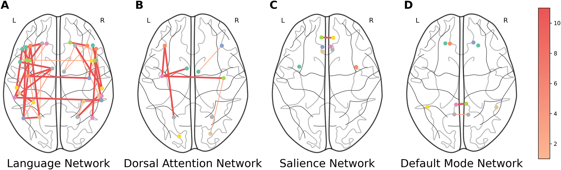
Selected rsFMRI-FC pairs for SVR. Thicker and darker lines between two ROIs indicate more frequent selection of functional connectivity between these regions. The color bar indicates the number of times a connection is selected (1–11). rsFMRI-FC: Resting State Functional Connectivity; SVR: Support Vector Regression.

Figure 9:

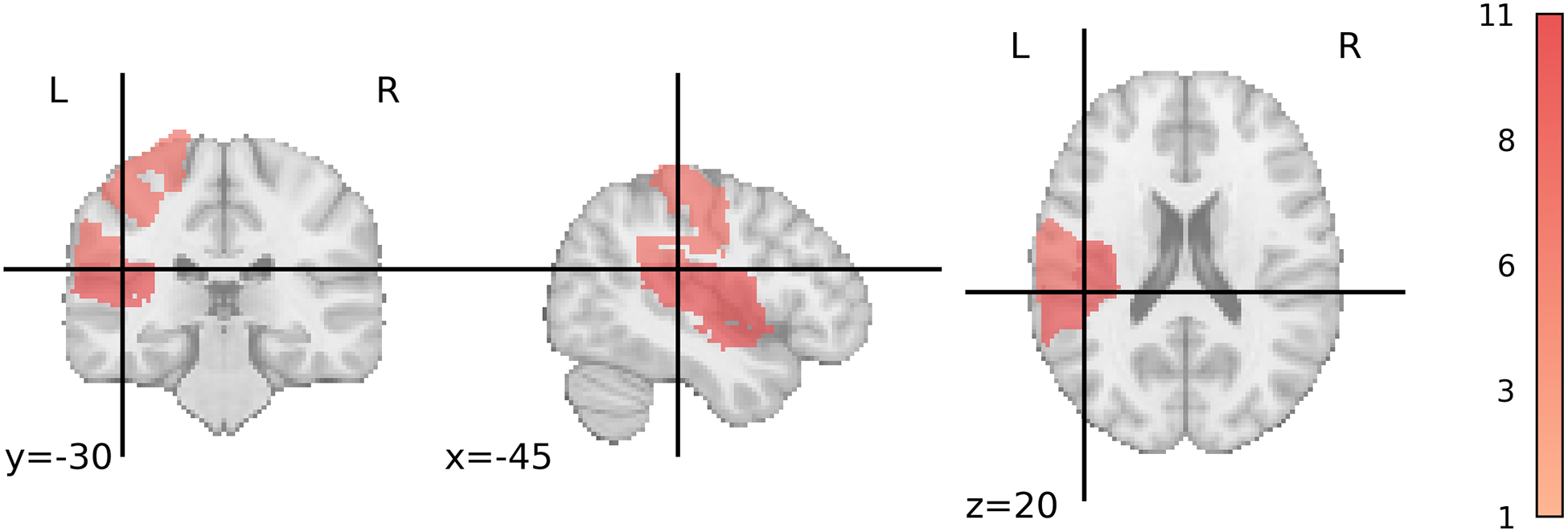
Selected PSG regions for SVR. Darker areas indicate more frequent selection of the region. The color bar indicates the number of times a region is selected (1–11). PSG: Percent Spared Grey Matter; SVR: Support Vector Regression.

The top 2 most frequently selected PSW features are the Fronto Insular tracts, and Arcuate Posterior Segment Left (Table 3). The Left Arcuate Fasciculus, Left Uncinate Fasciculus, Left Inferior Fronto-Occipital Fasciculus, and Left Inferior Longitudinal Fasciculus were the only selected features for FA (Table 3).

Table 3:

Feature Selection Frequencies for PSW and FA. Features with a selection frequency greater than 2 are shown.

Model Type	Predictor	Feature	Frequency
SVR	PSW	Fronto Insular tract5 Left	11
		Arcuate Posterior Segment Left	11
SVR	FA	Left Arcuate Fasciculus	11
		Left Uncinate Fasciculus	11
		Left Inferior Fronto-Occipital Fasciculus	10
		Left Inferior Longitudinal Fasciculus	10

PSW: Percent Spared White Matter; FA: Fractional Anisotropy; SVR: Support Vector Regression.

3.3. Resting-state Functional Connectivity

Notably, in both the RF and SVR models, the predictor rsFMRI-FC emerges as a crucial feature, significantly contributing to model performance. This can be discerned by analyzing the SHAP value ϕ_i for each predictor i and the distribution of marginal contributions $\left\{v\left(S\right)-v\left(S\cup \left\{i\right\}\right)\right\}$ across all subsets S of predictors that exclude predictor i (see Equation (1)). The SHAP values and distributions of marginal contributions for all individual predictors are in shown in Supplementary Table S3 and Figure S2. In the SVR model, rsFMRI-FC has the highest SHAP value of 3.65, indicating that it positively influences the model’s predictions, enhancing accuracy.

The consistent positive contribution of rsFMRI-FC highlights its robustness and importance. In fact, Figure 7 shows that rsFMRI-FC combined with the structural information consistently attains the lowest RSME scores.

3.4. Severe Case Limitations

Finally, neither SVR nor RF models are able to predict a small subset of patients with WAB-R AQ scores lower than 20 (N = 3) (Figures 10 and Supplementary Figure S6). A possible explanation for this could be the imbalanced distribution of WAB-R AQ scores, with fewer patients having severe aphasia compared to those with mild or moderate levels, resulting in comparatively less information about the severe group.

Figure 10:

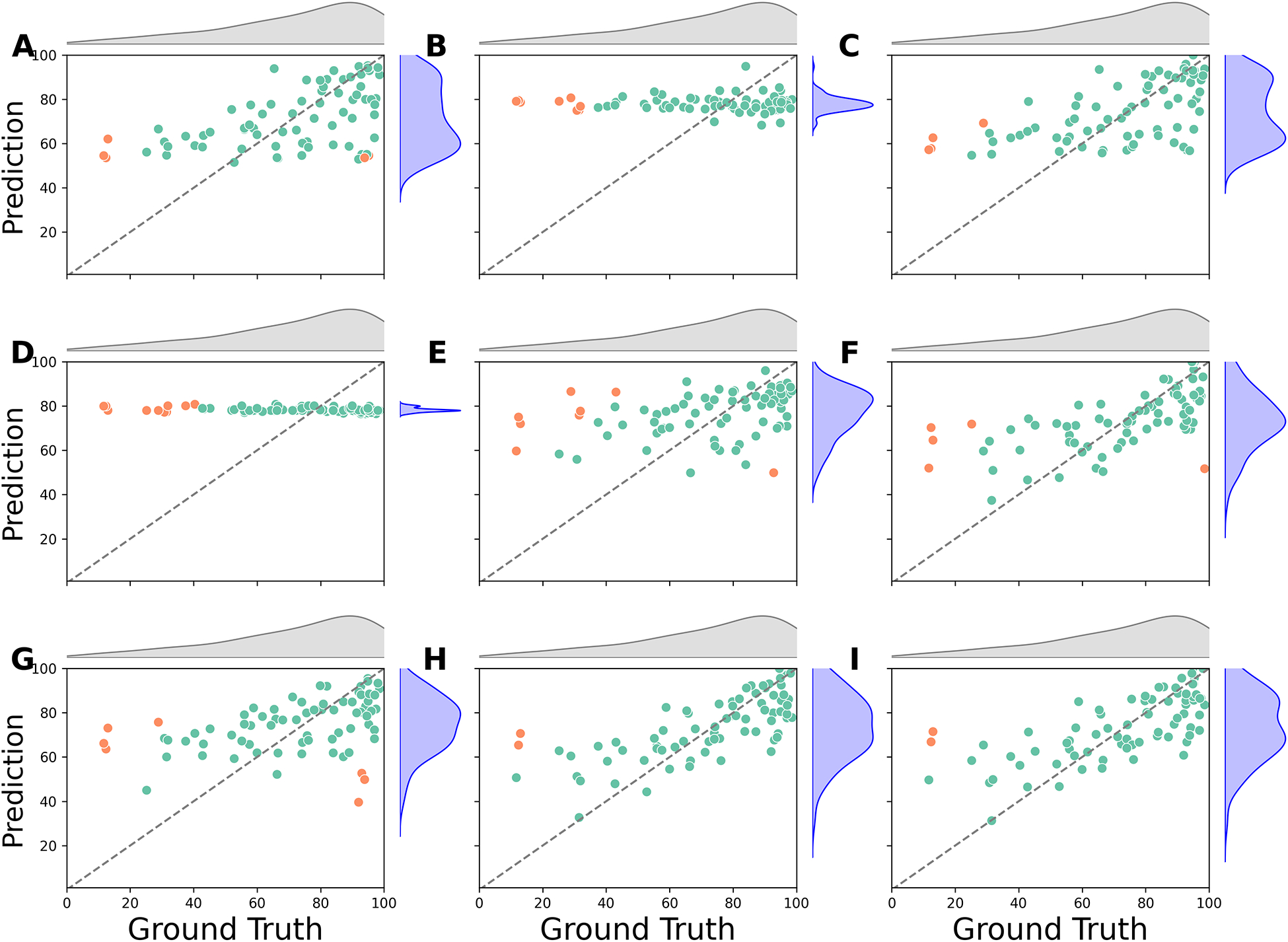
SVR Predictions vs. Ground Truth. The scatter plots compare the ground truth scores (horizontal axis) with the predicted scores (vertical axis). Points with a prediction error greater than 40 points are marked in orange. (A) PSW; (B) rsFMRI-trans; (C) PSG; (D) DM; (E) FA; (F) rsFMRI-FC; (G) LV; (H) Lowest RMSE (DM+PSW+rsFMRI-FC); (I) All predictors. rsFMRI-FC: Resting State Functional Connectivity; rsFMRI-trans: Resting State Transitivity; PSG: Percent Spared Grey Matter; PSW: Percent Spared White Matter; LV: Lesion Volume; FA: Fractional Anisotropy; DM: Demographic; SVR: Support Vector Regression.

4. Discussion

Overall, our results show that the SVR model consistently outperforms the RF model in predicting WAB-R AQ. Features selected by the RFE method provide valuable insights into understanding aphasia recovery. Second, integrating functional integrity, such as resting-state functional connectivity (rsFMRI-FC) with structural integrity (PSW/PSG) improves model performance compared to using single modalities alone. We discuss each of these results in detail below.

4.1. Comparisons between models

With our dataset, RF models were generally less accurate in predicting WAB-AQ scores compared to SVR models, which were better at utilizing the available data to predict scores accurately. As a result we focused our paper on the SVR results, but some theoretical and practical differences are worth pointing out. First, SVR is an extension of Support Vector Machines designed for regression tasks. SVR fits a linear or kernel regression model to given data by minimizing the so-called ϵ-insensitive loss. Essentially, SVR minimizes MAE ignoring absolute errors smaller than a threshold ϵ, and incorporates quadratic regularization for model parameters during training (Smola and Schölkopf, 2004). The threshold ϵ is a hyperparameter which is chosen during model training and tuning using samples in the validation-training folds.

On the other hand, RF models are a type of ensemble learning method that leverage the principles of bagging (bootstrap aggregating) to enhance predictive performance. In bagging, multiple subsets of the training data are created by sampling with replacement, and each subset is used to train a separate model. For RFs, these models are decision trees that each learn slightly different aspects of the data due to variations in their training subsets. The final prediction from an RF model is generated by averaging the outputs of all individual trees for regression (Breiman, 2001).

Results show that, for the data used in this study, the SVR model generates a lower average RMSE than the RF model. This finding indicates that SVR is more efficient at leveraging information unique to functional resting-state activity and complementary information from different predictors (Figure 4b). Similar results, where SVR outperforms RF, have been reported in other studies on aphasia recovery as well (Billot et al., 2022; Chennuri et al., 2023). The comparatively poorer performance of the RF model may be due to limitations in its structure.

Furthermore, the consistent observation that the RBF kernel achieved lower RMSE than the linear kernel for models combining rsFMRI-FC with PSW/PSG predictors suggests the presence of a non-linear relationship between rsFMRI-FC and PSW/PSG. This indicates that linear models may not fully capture the complexity of the interactions between these variables and underscores the need to account for non-linear relationships in neuroimaging data to improve predictive accuracy.

4.2. Features important to aphasia severity

The supervised feature selection method identified important features of overall language impairment. RFE with repeated cross-validation selects the top features that consistently have high feature importance for the given machine learning model. Nonetheless, selected rsFMRI-FC features for SVR models revealed that functional activation within the language network in both hemispheres and between homologous language regions consistently provided important information about aphasia severity. These results align with findings from previous studies. For example, Tao and Rapp (2020) found that increases in ipsilateral and homotopic connectivity were associated with improvements in treatment-driven spelling performance. In another study, Hope et al. (2017) observed that functional enhancements in various right hemisphere regions were linked to both improvements and declines in language skills, highlighting the complex role these areas play in recovery. Additionally, Elkana et al. (2013) noted that recovery was associated with increased functional activation in right hemisphere homologues of left hemisphere language regions. Together, these studies suggest that resting-state data offers valuable insights into brain functional reorganization, highlighting the importance of the bilateral residual language network.

In addition to rsFMRI-FC features, RFE identified PSG features in the left hemisphere language area as informative. Furthermore, the percentage of spared white matter tracts in the left hemisphere, particularly the arcuate fasciculus and fronto-insular tracts, was frequently selected by the feature selection method. Previous literature also underscores the importance of these tracts in language functioning. Previous studies have highlighted the crucial role of specific white matter tracts in language processing. For instance, Fridriksson et al. (2013) emphasized that damage to the anterior segment of the left arcuate fasciculus is a strong predictor of language fluency. Similarly, Basilakos et al. (2014) found that both the anterior segment of the arcuate fasciculus and the arcuate fasciculus as a whole influence speech production. Furthermore, voxel-based lesion-symptom mapping analysis, using T1-weighted and diffusion data, identified regions around the insula as areas with the highest lesion overlap when predicting aphasia recovery (Forkel and Catani, 2018). These structural findings are also complemented by functional neuroimaging studies. For example, using fMRI analysis, Oh et al. (2014) discovered that different regions within the insula play distinct roles in language outcomes.

Figure 7 illustrates the mean RMSE for SVR models, highlighting the impact of combining functional and structural integrity information. The horizontal axis shows model rankings based on mean RMSE, ordered from worst to best from left to right, while the vertical axis indicates the mean RMSE values. In the plot, a solid green rectangle at the bottom right (low RMSE) highlights the best-performing models, which combine both rsFMRI-FC and structural information (PSW or PSG). In contrast, models that exclude rsFMRI-FC and key structural predictors are located on the top left (higher RMSE) within a solid pink rectangle, indicating these as the worst-performing models. Dashed horizontal lines show the mean RMSE for models using only rsFMRI-FC (in orange) and PSG (in gray), providing reference benchmarks. The plot underscores the importance of integrating rsFMRI-FC with structural information to optimize model performance and outperform models that rely on only one type of information. It is worth noting that these findings are replicated with the RF models shown in the supplemental section.

Furthermore, rsFMRI-FC has high positive SHAP values in both model types (Supplementary Table S3 and Figure S2), indicating that it makes a significant positive contribution to the model’s predictions when combined with other predictors. Collectively, these results across both models suggest that an integrated set of features combining both structural and functional integrity yields the lowest RMSE values, consistently appears in the top models, and best predicts aphasia severity.

The significantly better prediction with combined rsFMRI-FC and structural integrity information suggests that combining functional and structural information provides a more comprehensive view of the brain’s architecture and its dynamic function, leading to a fuller picture of the brain’s state and potential. The superiority of integrated models can be explained by the complex interplay between brain structure and function. Structural damage in specific brain areas might disrupt functional networks that span distant regions, a phenomenon that becomes apparent only when both data types are analyzed together. This synergy between structural and functional data allows for a more nuanced understanding of language impairments and recovery pathways.

4.3. Limitations and Future Research

Our research faces limitations due to the small sample size of multimodal imaging data, despite adequately representing aphasia patient heterogeneity, and the greater number of male compared to female participants, which could bias the results. To address the imbalance between numerous features and limited samples, we employed supervised feature selection and nested cross-validation, enhancing model accuracy and generalizability. However, our models struggle to predict outcomes for severe aphasia patients (WAB-R AQ scores below 20), as the SVR model fails to capture nuances of smaller, distinct subgroups without sufficient information. Research by Teghipco et al. (2024) has shown extensive brain morphometry differences in severe aphasia patients, further complicating accurate predictions for this group. Although our dataset represents various aphasia severity levels (see Supplementary Table S4), the standard SVR model’s structure limits its ability to effectively capture patterns within minority classes, resulting in less accurate predictions for severe cases.

Another limitation of this study is that data from Cohort 1 and Cohort 2 were processed using different pipelines for both lesion segmentation and DTI preprocessing. For lesion segmentation, Cohort 1 lesions were identified using a semi-automated method in ITK-SNAP, while Cohort 2 lesions were manually traced using MRIcron. This difference reflects the time at which the datasets were collected, as the ITK-SNAP pipeline had not yet been validated within our research group during the acquisition of Cohort 2. While both approaches are commonly used in stroke research, differences in lesion delineation methodology may introduce variability in lesion-based features such as percent spared gray and white matter. Regarding DTI preprocessing, some raw diffusion files were missing for participants in Cohort 2, which prevented us from reprocessing all DTI data through a unified pipeline. This discrepancy may have contributed to the relatively weaker predictive contribution of fractional anisotropy (FA) in our models. Nonetheless, the distribution of FA values between the two cohorts was largely similar (see Supplementary Figure S1), suggesting that any resulting bias was likely minimal.

Future research should explore alternative predictors to enhance model performance and deepen our understanding of aphasia’s neural substrates. Exploring a wider range of connectivity measures beyond the subset of whole-brain resting-state connectivity matrix and transitivity scores used in this study could provide valuable insights. However, we included rsFMRI transitivity as a measure, which was not important. Furthermore, future studies could consider integrating additional modalities and extracting novel types of information, such as brain morphometry data, especially from the right hemisphere. This approach is supported by previous literature highlighting the relationship between right hemisphere gray matter volumes and language abilities (Lukic et al., 2017; Xing et al., 2016), as well as recent findings by Teghipco et al. (2024) using convolutional neural networks to predict severe aphasia.

In conclusion, SVR models accurately (and better than RF models) leverage unique information in resting-state connectivity and complementary information from modalities to predict WAB-R-AQ. The supervised feature selection method reveals that functional connectivity in both hemispheres and between homologous language areas is critical for predicting language outcomes in aphasia patients. These findings indicate that language outcomes are influenced by factors beyond just the lesion location and lesion volume, and combining different modalities provides a more comprehensive understanding of brain dynamics and neuroplasticity. Modeling the brain structural and functional features that predict severity is the first step towards predicting potential recovery in PWA once we understand their starting point prior to therapy.

Highlights.

• Combining information about structural and functional integrity improves aphasia severity prediction.

• Support Vector Regression outperformed Random Forest in predicting aphasia severity.

• Functional connectivity in bilateral language regions predicts aphasia severity.

References

- Ashburner J, 2007. A fast diffeomorphic image registration algorithm. Neuroimage 38, 95–113. [DOI] [PubMed] [Google Scholar]
- Ashburner J, Friston KJ, 2005. Unified segmentation. Neuroimage 26, 839–851. [DOI] [PubMed] [Google Scholar]
- Awad M, Khanna R, 2015. Support vector regression, in: Efficient Learning Machines. Apress, Berkeley, CA, pp. 67–80. [Google Scholar]
- Basilakos A, Fillmore PT, Rorden C, Guo D, Bonilha L, Fridriksson J, 2014. Regional White Matter Damage Predicts Speech Fluency in Chronic Post-Stroke Aphasia. Frontiers in Human Neuroscience 8. doi: 10.3389/fnhum.2014.00845. publisher: Frontiers. [DOI] [PMC free article] [PubMed] [Google Scholar]
- Billot A, Lai S, Varkanitsa M, Braun EJ, Rapp B, Parrish TB, Higgins J, Kurani AS, Caplan D, Thompson CK, Ishwar P, Betke M, Kiran S, 2022. Multimodal Neural and Behavioral Data Predict Response to Rehabilitation in Chronic Poststroke Aphasia. Stroke 53, 1606–1614. doi: 10.1161/STROKEAHA.121.036749. publisher: American Heart Association. [DOI] [PMC free article] [PubMed] [Google Scholar]
- Braun E, Billot A, Meier E, 2022. White matter microstructural integrity pre- and post-treatment in individuals with chronic post-stroke aphasia. Brain Lang 232. doi: 10.1016/j.bandl.2022.105163. [DOI] [PMC free article] [PubMed] [Google Scholar]
- Breiman L, 2001. Random Forests. Machine Learning 45, 5–32. doi: 10.1023/A:1010933404324. [DOI] [Google Scholar]
- Chai T, Draxler RR, 2014. Root mean square error (RMSE) or mean absolute error (MAE)? – Arguments against avoiding RMSE in the literature. Geoscientific Model Development 7, 1247–1250. doi: 10.5194/gmd-7-1247-2014. publisher: Copernicus GmbH. [DOI] [Google Scholar]
- Chennuri S, Lai S, Billot A, Varkanitsa M, Braun EJ, Kiran S, Venkataraman A, Konrad J, Ishwar P, Betke M, 2023. Fusion Approaches to Predict Post-stroke Aphasia Severity from Multimodal Neuroimaging Data, in: 2023 IEEE/CVF International Conference on Computer Vision Workshops (ICCVW), IEEE, Paris, France. pp. 2636–2645. doi: 10.1109/ICCVW60793.2023.00279. [DOI] [Google Scholar]
- Cook PA, Bai Y, Nedjati-Gilani S, Seunarine KK, Hall MG, Parker GJ, Alexander DC, 2006. Camino: Open-Source Diffusion-MRI Reconstruction and Processing, in: Proceedings of the 14th Scientific Meeting of the International Society for Magnetic Resonance in Medicine, Seattle, WA, USA. p. 2759. [Google Scholar]
- Crosson B, Rodriguez AD, Copland D, Fridriksson J, Krishnamurthy LC, Meinzer M, Raymer AM, Krishnamurthy V, Leff AP, 2019. Neuroplasticity and aphasia treatments: new approaches for an old problem. Journal of Neurology, Neurosurgery & Psychiatry 90, 1147–1155. doi: 10.1136/jnnp-2018-319649. publisher: BMJ Publishing Group Ltd Section: Cognitive neurology. [DOI] [PMC free article] [PubMed] [Google Scholar]
- Demircioğlu A, 2024. The effect of feature normalization methods in radiomics. Insights into Imaging 15, 2. URL: https://doi.org/10.1186/s13244-023-01575-7, doi: 10.1186/s13244-023-01575-7. [DOI] [PMC free article] [PubMed] [Google Scholar]
- Elkana O, Frost R, Kramer U, Ben-Bashat D, Schweiger A, 2013. Cerebral language reorganization in the chronic stage of recovery: a longitudinal fMRI study. Cortex; a Journal Devoted to the Study of the Nervous System and Behavior 49, 71–81. doi: 10.1016/j.cortex.2011.09.001. [DOI] [PubMed] [Google Scholar]
- Falconer I, Varkanitsa M, Kiran S, 2024. Resting-state brain network connectivity is an independent predictor of responsiveness to language therapy in chronic post-stroke aphasia. Cortex 173, 296–312. doi: 10.1016/j.cortex.2023.11.022. [DOI] [PMC free article] [PubMed] [Google Scholar]
- Forkel SJ, Catani M, 2018. Lesion mapping in acute stroke aphasia and its implications for recovery. Neuropsychologia 115, 88–100. doi: 10.1016/j.neuropsychologia.2018.03.036. [DOI] [PMC free article] [PubMed] [Google Scholar]
- Forkel SJ, Thiebaut De Schotten M, Dell’Acqua F, Kalra L, Murphy DGM, Williams SCR, Catani M, 2014. Anatomical predictors of aphasia recovery: a tractography study of bilateral perisylvian language networks. Brain 137, 2027–2039. doi: 10.1093/brain/awu113. [DOI] [PubMed] [Google Scholar]
- Foulon C, Cerliani L, Kinkingnéhun S, Levy R, Rosso C, Urbanski M, Volle E, Thiebaut de Schotten M, 2018. Advanced lesion symptom mapping analyses and implementation as BCBtoolkit. GigaScience 7, giy004. doi: 10.1093/gigascience/giy004. [DOI] [PMC free article] [PubMed] [Google Scholar]
- Fridriksson J, Guo D, Fillmore P, Holland A, Rorden C, 2013. Damage to the anterior arcuate fasciculus predicts non-fluent speech production in aphasia. Brain 136, 3451–3460. doi: 10.1093/brain/awt267. [DOI] [PMC free article] [PubMed] [Google Scholar]
- Fridriksson J, Yourganov G, Bonilha L, Basilakos A, Den Ouden DB, Rorden C, 2016. Revealing the dual streams of speech processing. Proceedings of the National Academy of Sciences 113, 15108–15113. doi: 10.1073/pnas.1614038114. publisher: Proceedings of the National Academy of Sciences. [DOI] [PMC free article] [PubMed] [Google Scholar]
- Friedman JW, 1986. Game theory with applications to economics. New York:Oxford University Press. [Google Scholar]
- Friston KJ, Ashburner J, Frith CD, Poline JB, Heather JD, Frackowiak RS, 1995. Spatial registration and normalization of images. Human brain mapping 3, 165–189. [Google Scholar]
- Gaizo JD, Fridriksson J, Yourganov G, Hillis AE, Hickok G, Misic B, Rorden C, Bonilha L, 2017. Mapping Language Networks Using the Structural and Dynamic Brain Connectomes. eNeuro 4. doi: 10.1523/ENEURO.0204-17.2017. publisher: Society for Neuroscience Section: Methods/New Tools. [DOI] [PMC free article] [PubMed] [Google Scholar]
- Geller J, Thye M, Mirman D, 2019. Estimating effects of graded white matter damage and binary tract disconnection on post-stroke language impairment. NeuroImage 189, 248–257. doi: 10.1016/j.neuroimage.2019.01.020. [DOI] [PubMed] [Google Scholar]
- Gilmore N, Meier E, Johnson J, Kiran S, 2020. Typicality-based semantic treatment for anomia results in multiple levels of generalisation. Neuropsychol Rehabil 30, 802–828. doi: 10.1080/09602011.2018.1499533. [DOI] [PMC free article] [PubMed] [Google Scholar]
- Grönberg A, Henriksson I, Stenman M, Lindgren AG, 2022. Incidence of Aphasia in Ischemic Stroke. Neuroepidemiology 56, 174–182. doi: 10.1159/000524206. [DOI] [PubMed] [Google Scholar]
- Guyon I, Weston J, Barnhill S, Vapnik V, 2002. Gene Selection for Cancer Classification using Support Vector Machines. Machine Learning 46, 389–422. doi: 10.1023/A:1012487302797. [DOI] [Google Scholar]
- Halai AD, Woollams AM, Lambon Ralph MA, 2020. Investigating the effect of changing parameters when building prediction models for post-stroke aphasia. Nature Human Behaviour 4, 725–735. doi: 10.1038/s41562-020-0854-5. [DOI] [PMC free article] [PubMed] [Google Scholar]
- Hope TMH, Leff AP, Prejawa S, Bruce R, Haigh Z, Lim L, Ramsden S, Oberhuber M, Ludersdorfer P, Crinion J, Seghier ML, Price CJ, 2017. Right hemisphere structural adaptation and changing language skills years after left hemisphere stroke. Brain 140, 1718–1728. doi: 10.1093/brain/awx086. [DOI] [PMC free article] [PubMed] [Google Scholar]
- Hope TMH, Leff AP, Price CJ, 2018. Predicting language outcomes after stroke: Is structural disconnection a useful predictor? NeuroImage: Clinical 19, 22–29. doi: 10.1016/j.nicl.2018.03.037. [DOI] [PMC free article] [PubMed] [Google Scholar]
- Hope TMH, Seghier ML, Leff AP, Price CJ, 2013. Predicting outcome and recovery after stroke with lesions extracted from MRI images. NeuroImage: Clinical 2, 424–433. doi: 10.1016/j.nicl.2013.03.005. [DOI] [PMC free article] [PubMed] [Google Scholar]
- Johnson J, Meier E, Pan Y, Kiran S, 2019. Treatment-related changes in neural activation vary according to treatment response and extent of spared tissue in patients with chronic aphasia. Cortex 121, 147–168. doi: 10.1016/j.cortex.2019.08.016. [DOI] [PMC free article] [PubMed] [Google Scholar]
- Johnson J, Meier E, Pan Y, Kiran S, 2020. Pre-treatment graph measures of a functional semantic network are associated with naming therapy outcomes in chronic aphasia. Brain Lang 207. doi: 10.1016/j.bandl.2020.104809. [DOI] [PMC free article] [PubMed] [Google Scholar]
- Johnson J, Meier E, Pan Y, Kiran S, 2021. Abnormally weak functional connections get stronger in chronic stroke patients who benefit from naming therapy. Brain Lang 223. doi: 10.1016/j.bandl.2021.105042. [DOI] [PMC free article] [PubMed] [Google Scholar]
- Kertesz A, 2012. Western Aphasia Battery–Revised. doi: 10.1037/t15168-000. institution: American Psychological Association. [DOI] [Google Scholar]
- Kristinsson S, Zhang W, Rorden C, Newman-Norlund R, Basilakos A, Bonilha L, Yourganov G, Xiao F, Hillis A, Fridriksson J, 2020. Machine learning-based multimodal prediction of language outcomes in chronic aphasia. Human Brain Mapping 42, 1682–1698. doi: 10.1002/hbm.25321. [DOI] [PMC free article] [PubMed] [Google Scholar]
- Kuceyeski A, Navi BB, Kamel H, Raj A, Relkin N, Toglia J, Iadecola C, O’Dell M, 2016. Structural connectome disruption at baseline predicts 6-months post-stroke outcome. Human Brain Mapping 37, 2587–2601. doi: 10.1002/hbm.23198. [DOI] [PMC free article] [PubMed] [Google Scholar]
- Lam JMC, Wodchis WP, 2010. The relationship of 60 disease diagnoses and 15 conditions to preference-based health-related quality of life in Ontario hospital-based long-term care residents. Medical Care 48, 380–387. doi: 10.1097/MLR.0b013e3181ca2647. [DOI] [PubMed] [Google Scholar]
- Li L, Scott CA, Rothwell PM, on behalf of the Oxford Vascular Study, 2020. Trends in Stroke Incidence in High-Income Countries in the 21st Century. Stroke 51, 1372–1380. doi: 10.1161/STROKEAHA.119.028484. publisher: American Heart Association. [DOI] [PMC free article] [PubMed] [Google Scholar]
- Lo A, Chernoff H, Zheng T, Lo SH, 2015. Why significant variables aren’t automatically good predictors. Proceedings of the National Academy of Sciences of the United States of America 112, 13892–13897. doi: 10.1073/pnas.1518285112. [DOI] [PMC free article] [PubMed] [Google Scholar]
- Lukic S, Barbieri E, Wang X, Caplan D, Kiran S, Rapp B, Parrish TB, Thompson CK, 2017. Right Hemisphere Grey Matter Volume and Language Functions in Stroke Aphasia. Neural Plasticity 2017, 5601509. doi: 10.1155/2017/5601509. [DOI] [PMC free article] [PubMed] [Google Scholar]
- Meier E, Johnson J, Pan Y, Kiran S, 2019a. A lesion and connectivity-based hierarchical model of chronic aphasia recovery dissociates patients and healthy controls. NeuroImage Clin 23. doi: 10.1016/j.nicl.2019.101919. [DOI] [PMC free article] [PubMed] [Google Scholar]
- Meier E, Johnson J, Pan Y, Kiran S, 2019b. The utility of lesion classification models in predicting language abilities and treatment outcomes in persons with aphasia. Brain Imaging Behav 13, 1510–1525. doi: 10.3389/conf.fnhum.2018.228.00083. [DOI] [PMC free article] [PubMed] [Google Scholar]
- Modig K, Talbäck M, Ziegler L, Ahlbom A, 2019. Temporal trends in incidence, recurrence and prevalence of stroke in an era of ageing populations, a longitudinal study of the total Swedish population. BMC Geriatrics 19, 31. doi: 10.1186/s12877-019-1050-1. [DOI] [PMC free article] [PubMed] [Google Scholar]
- Nieto-Castanon A, 2020. Fmri minimal preprocessing pipeline, in: Handbook of functional connectivity Magnetic Resonance Imaging methods in CONN. Hilbert Press, pp. 3–16. [Google Scholar]
- Nieto-Castanon A, 2022. Preparing fmri data for statistical analysis. arXiv URL: https://arxiv.org/abs/2210.13564, arXiv:2210.13564. [Google Scholar]
- Oh A, Duerden EG, Pang EW, 2014. The role of the insula in speech and language processing. Brain and language 135, 96–103. doi: 10.1016/j.bandl.2014.06.003. [DOI] [PMC free article] [PubMed] [Google Scholar]
- Pedregosa F, Varoquaux G, Gramfort A, Michel V, Thirion B, Grisel O, Blondel M, Prettenhofer P, Weiss R, Dubourg V, Vanderplas J, Passos A, Cournapeau D, Brucher M, Perrot M, Duchesnay E, 2011. Scikit-learn: Machine learning in Python. Journal of Machine Learning Research 12, 2825–2830. [Google Scholar]
- Power JD, Mitra A, Laumann TO, Snyder AZ, Schlaggar BL, Petersen SE, 2014. Methods to detect, characterize, and remove motion artifact in resting state fmri. Neuroimage 84, 320–341. [DOI] [PMC free article] [PubMed] [Google Scholar]
- Pustina D, Coslett HB, Ungar L, Faseyitan OK, Medaglia JD, Avants B, Schwartz MF, 2017. Enhanced estimations of post-stroke aphasia severity using stacked multimodal predictions. Human Brain Mapping 38, 5603–5615. doi: 10.1002/hbm.23752. [DOI] [PMC free article] [PubMed] [Google Scholar]
- Ramsey LE, Siegel JS, Lang CE, Strube M, Shulman GL, Corbetta M, 2017. Behavioural clusters and predictors of performance during recovery from stroke. Nature Human Behaviour 1, 0038. doi: 10.1038/s41562-016-0038. [DOI] [PMC free article] [PubMed] [Google Scholar]
- Rojkova K, Volle E, Urbanski M, Humbert F, Dell’Acqua F, Thiebaut de Schotten M, 2016. Atlasing the frontal lobe connections and their variability due to age and education: a spherical deconvolution tractography study. Brain Structure and Function 221, 1751–1766. doi: 10.1007/s00429-015-1001-3. [DOI] [PubMed] [Google Scholar]
- Rolls ET, Huang CC, Lin CP, Feng J, Joliot M, 2020. Automated anatomical labelling atlas 3. NeuroImage 206, 116189. doi: 10.1016/j.neuroimage.2019.116189. [DOI] [PubMed] [Google Scholar]
- Rubinov M, Kötter R, Hagmann P, Sporns O, 2009. Brain connectivity toolbox: a collection of complex network measurements and brain connectivity datasets. NeuroImage 47, S169. doi: 10.1016/S1053-8119(09)71822-1. [DOI] [Google Scholar]
- Smola AJ, Schölkopf B, 2004. A tutorial on support vector regression. Statistics and Computing 14, 199–222. URL: https://doi.org/10.1023/B:STCO.0000035301.49549.88, doi: 10.1023/B:STCO.0000035301.49549.88. [DOI] [Google Scholar]
- Tao Y, Rapp B, 2020. How functional network connectivity changes as a result of lesion and recovery: An investigation of the network phenotype of stroke. Cortex; a journal devoted to the study of the nervous system and behavior 131, 17–41. doi: 10.1016/j.cortex.2020.06.011. [DOI] [PMC free article] [PubMed] [Google Scholar]
- Teghipco A, Newman-Norlund R, Fridriksson J, Rorden C, Bonilha L, 2024. Distinct brain morphometry patterns revealed by deep learning improve prediction of post-stroke aphasia severity. Communications Medicine 4, 115. doi: 10.1038/s43856-024-00541-8. [DOI] [PMC free article] [PubMed] [Google Scholar]
- Virtanen P, Gommers R, Oliphant TE, Haberland M, Reddy T, Cournapeau D, Burovski E, Peterson P, Weckesser W, Bright J, van der Walt SJ, Brett M, Wilson J, Millman KJ, Mayorov N, Nelson ARJ, Jones E, Kern R, Larson E, Carey CJ, Polat İ, Feng Y, Moore EW, VanderPlas J, Laxalde D, Perktold J, Cimrman R, Henriksen I, Quintero EA, Harris CR, Archibald AM, Ribeiro AH, Pedregosa F, van Mulbregt P, SciPy 1.0 Contributors, 2020. SciPy 1.0: Fundamental Algorithms for Scientific Computing in Python. Nature Methods 17, 261–272. doi: 10.1038/s41592-019-0686-2. [DOI] [PMC free article] [PubMed] [Google Scholar]
- Wang J, Marchina S, Norton AC, Wan CY, Schlaug G, 2013. Predicting speech fluency and naming abilities in aphasic patients. Frontiers in Human Neuroscience 7, 831. doi: 10.3389/fnhum.2013.00831. [DOI] [PMC free article] [PubMed] [Google Scholar]
- Whitfield-Gabrieli S, Nieto-Castanon A, Ghosh S, 2011. Artifact detection tools (ART). Technical Report. Cambridge, MA Release Version, 7(19), 11. [Google Scholar]
- Xing S, Lacey EH, Skipper-Kallal LM, Jiang X, Harris-Love ML, Zeng J, Turkeltaub PE, 2016. Right hemisphere grey matter structure and language outcomes in chronic left hemisphere stroke. Brain 139, 227–241. doi: 10.1093/brain/awv323. [DOI] [PMC free article] [PubMed] [Google Scholar]
- Yourganov G, Fridriksson J, Rorden C, Gleichgerrcht E, Bonilha L, 2016. Multivariate Connectome-Based Symptom Mapping in Post-Stroke Patients: Networks Supporting Language and Speech. Journal of Neuroscience 36, 6668–6679. doi: 10.1523/JNEUROSCI.4396-15.2016. publisher: Society for Neuroscience Section: Articles. [DOI] [PMC free article] [PubMed] [Google Scholar]
- Yourganov G, Fridriksson J, Stark B, Rorden C, 2018. Removal of artifacts from resting-state fMRI data in stroke. NeuroImage: Clinical 17, 297–305. doi: 10.1016/j.nicl.2017.10.027. [DOI] [PMC free article] [PubMed] [Google Scholar]
- Yourganov G, Smith KG, Fridriksson J, Rorden C, 2015. Predicting aphasia type from brain damage measured with structural MRI. Cortex 73, 203–215. doi: 10.1016/j.cortex.2015.09.005. [DOI] [PMC free article] [PubMed] [Google Scholar]
- Yushkevich P, Piven J, Hazlett H, 2006. User-guided 3d active contour segmentation of anatomical structures: Significantly improved efficiency and reliability. Neuroimage 31, 1116–1128. doi: 10.1016/j.neuroimage.2006.01.015. [DOI] [PubMed] [Google Scholar]
Associated Data
This section collects any data citations, data availability statements, or supplementary materials included in this article.