Self-assembly of a metal-ion-bound monolayer of trigonal connectors on mercury: An electrochemical Langmuir trough

Abstract

The adsorption of the trigonal connector, 1,3,5-tris[10-(3-ethylthiopropyl)dimethylsilyl-1,10-dicarba-closo-decaboran-1-yl]benzene (1), from acetonitrile/0.1 M LiClO₄ on the surface of mercury at potentials ranging from +0.3 to −1.4 V (vs. aqueous Ag|AgCl|1 M LiCl) was examined by voltammetry, Langmuir isotherms at controlled potentials, and impedance measurements. No adsorption is observed at potentials more negative than ∼ −0.85 V. Physisorption is seen between ∼ −0.85 and 0 V. At positive potentials, adsorbate-assisted anodic dissolution of mercury occurs and an organized surface layer is formed. Although the mercury cations are reduced at −0.10 V, the surface layer remains metastable to potentials as negative as −0.85 V. Its surface areas per molecule and per redox center are compatible with a regular structure with the connectors 1 woven into a hexagonal network by RR′S→Hg←SRR′ or RR′S→Hg²⁺←SRR′ bridges. The structure is simulated closely by geometry optimization in the semiempirical AM1 approximation.

Elsewhere in this issue (1) we outline the motivation for our efforts to prepare extended regular grids on the surface of mercury by reversible self-assembly. Here, we describe an electrochemical Langmuir trough for the determination of a surface molecular area at the interface of mercury and an electrolyte solution at a controlled potential. We use it to shed light on the possible formation of a two-dimensional hexagonal grid by the binding of trigonal connectors to each other through a mutual coupling of their thioether-containing arm terminals by means of ligation to mercury cations.

It has been long known (2) that anodic dissolution of mercury is facilitated by the presence of species with a large affinity for mercury ions. These can be anions, such as oxalate (3, 4), or neutral ligands, such as azaaromatics (5). Sulfur compounds, especially sulfide and thiols, have attracted particular attention (6–16). Often, the mercury-ion-containing salts adhere firmly to the mercury surface in the form of highly insoluble compact monolayers or multilayers. Although the mechanism of their formation has been much investigated (4, 5, 10, 11, 13, 17–24), structural information for these layers on mercury is limited except for the simplest cases, such as Hg₂Cl₂ (25, 26). The growth of two-dimensional crystals of salts of other metals on mercury surface is known (27, 28), and nucleation and growth phenomena in electrocrystallization have been reviewed recently (29). The mercury-adsorbed layers are compact, with lateral interactions among the adsorbed species essential for stability.

We have reported (30) the formation of such an adsorbed layer on a dropping mercury electrode from acetonitrile and dichloromethane solutions of a trigonal connector with a thioether link in each of its three arms, and suggested an open hexagonal grid structure for it. We now examine in more detail the properties of a monolayer formed from a similar connector that differs only by substitution of 10-vertex for 12-vertex carboranes in the three arms. The connector is 1,3,5-tris[10-(3-ethylthiopropyl)dimethylsilyl-1,10-dicarba-closo-decaboran-1-yl]benzene (1, Fig. 1); its synthesis and crystal structure have been completed (L.P., N.V., Z. Janoušek, B. Grüner, B. Wang, J. Pecka, R. M. Harrison, B. C. Noll, T.F.M., and J.M., unpublished results).

Figure 1.

Molecular structure of 1. The dots in the carborane cages stand for carbon atoms and the other vertices for BH groups.

In the previous work on the 12-vertex carborane analogue of 1, evidence for anodic dissolution of mercury was obtained from cyclic voltammetry, and formation of a strongly adsorbed monolayer was deduced from capacitance measurements. It was difficult to obtain reliable numbers for the surface area per molecule and per redox center from electrochemical measurements alone, and the electrochemical Langmuir trough represents a considerable advance. We originally estimated the number of electrons n exchanged per molecule by analyzing the height of the diffusion-controlled anodic peak as a function of solute concentration, assuming a reasonable value for the diffusion coefficient. For acetonitrile/LiClO₄, we found n equal to ∼2, which corresponds to no simple structure (when all three connector arms are used for cation binding, n should be 1.5 if the cation is singly charged and 3 if it is doubly charged). The accuracy of this determination was limited by low sample solubility and the resulting relatively large charging current, and by the tendency of the solute to adsorb on glass walls. Integration of the cathodic peak yielded 1.13 × 10⁻¹⁰ mol⋅cm⁻² as the maximum surface concentration of one-electron exchanging redox centers (which we unfortunately referred to as the concentration of 1), and 1.47 nm² as the area per one-electron redox center. Because we found n = ∼2, this translates into 2.94 nm² per molecule, clearly too small for a planar hexagonal grid. However, with tetrabutylammonium hexafluorophosphate as supporting electrolyte in acetonitrile or dichloromethane, the maximum surface concentration was two and four times lower, respectively. In these cases, the hexagonal grid structure appeared possible (n = ∼1.5 was found, suggesting binding by means of Hg⁺ cations). Presently, we examine the acetonitrile/LiClO₄ solvent system on an electrochemical Langmuir trough, and find that the surface concentration of 1 in the monolayer fits expectations for the desired porous hexagonal grid.

Experimental Part

Molecular simulations used the titan program by Wavefunction (Irvine, CA; AM1 method; ref. 31).

Electrochemical measurements were made with a home-built system consisting of a fast rise-time potentiostat (32) and a lock-in amplifier (Stanford Research, Sunnyvale, CA; model SR830), interfaced to a personal computer via an IEEE-interface card (PC-Lab, AdvanTech, Irvine, CA; model PCL-848) and a data acquisition card (PCL-818) with 12-bit precision. The AC signal for the cell was derived from the internal oscillator of the lock-in amplifier (amplitude, 5 mV p–p). The electrochemical cell used an aqueous Ag|AgCl|1 M LiCl reference electrode separated from the test solution by a salt bridge (half-wave potential of ferrocene, +0.562 V; there were no indications of water penetrating into the system). A computer-triggered valve-operated glass-electrode static or hammer-dislodged dropping mercury working electrode (SMDE2, Laboratorní Pr̆ístroje, Prague, area 1.13 × 10⁻² cm²), and a cylindrical platinum net auxiliary electrode were used. The electrode was extruded into the solution within 50 ms, at a controlled potential. Measurements on the static electrode were started 4 s later, and it was verified that this waiting time was sufficient. Capacitance readings were taken in 1-s intervals on the static electrode and 40 ms before the end of drop life on the dropping electrode (4-s drop time). All measurements were performed in a 0.1 M solution of lithium perchlorate (Aldrich, vacuum-dried) in acetonitrile (Fluka, used as received), deoxygenated with a stream of argon. The saturated solution of 1 used in the measurements had a concentration between 100 and 160 μM.

Langmuir isotherms at a mercury–acetonitrile interface were measured with an instrument built for that purpose (Fig. 2) and housed under a dry nitrogen atmosphere in a glove box. The barrier driving system, surface balance, Wilhelmy plate, and software control were adopted from a computer-controlled KSV 5000 Langmuir–Blodgett trough. A rectangular electrically isolated stainless steel trough with inside dimensions of 40 cm × 4 cm and a height of 2 cm was filled with mercury from an attached reservoir. Flow of mercury between the trough and the reservoir was used to assure a fresh surface and to adjust the mercury level in the trough. An amalgamated copper bar served as the movable barrier. Copper was chosen because mercury wets it well, and the resulting convex shape of the meniscus at the barrier prevents any slippage of interface-adsorbed molecules under the barrier, which would be a concern with a concave meniscus. The disadvantage of copper is that it slowly accumulates in the mercury, which has to be periodically replaced. For cleaning, the mercury surface was swept with the barrier and contaminants were aspirated with a Pasteur pipette into a separatory funnel, from which mercury can be returned to the reservoir, whereas the supernatant waste is removed from the dry box. The mercury pool in the trough was covered with a 0.1 M solution of lithium perchlorate in deaerated acetonitrile. Surface pressure was measured with a platinum Wilhelmy plate attached to an electrobalance. The counterelectrode was a set of evenly distributed interconnected platinum wires immersed into the solution above the mercury surface. The electrical potential of the mercury was controlled with a CV-50W BAS potentiostat (BAS, West Lafayette, IN), connected to the trough through sealed leads. The reference electrode was Ag|0.01 M AgNO₃|0.1 M Bu₄NPF₆ in acetonitrile, but all potentials reported have been referred to the aqueous Ag|AgCl|1 M LiCl electrode by intermediacy of the ferrocene/ferricinium couple. For a measurement, a known amount of a 10 μM solution of 1 in acetonitrile was spread on the mercury pool and the solvent was evaporated, leaving behind a clear film free of any patches or specks. The electrolyte solution was added, and the desired potential was applied simultaneously. After a 2-min pause, the surface pressure–area isotherm was recorded by moving the barrier at 50 mm/min. At some potentials, the isotherms had the familiar shape, with a very slowly rising part at large surface areas and a rapidly rising part at smaller areas. In those cases, an area obtained by linear extrapolation of the steeply rising high-pressure part of the isotherm to zero pressure was plotted against the number of molecules of 1 in the monolayer. The plots were linear and their slopes were taken to correspond to areas per firmly adsorbed molecule. At other potentials, the isotherms lacked the steeply rising part, except at negligibly small surface areas, unrelated to the amount of 1 present and presumably caused by small amounts of impurities. There was very little resistance to compression, and no firmly adsorbed molecules (“zero area per molecule”).

Figure 2.

Schematic drawing of the electrochemical Langmuir trough.

In investigations of electrochemical hysteresis, the initial monolayer was equilibrated at a potential of +0.1 V for 2 min. The potential was then stepped to the desired value, and the system was rested for another 2 min before compression and isotherm recording.

Results

Cyclic Voltammetry.

Not surprisingly, cyclic voltammetry of 1 on a static mercury electrode yields results essentially identical to those found previously (30) in an examination of a very similar 12-vertex carborane analogue. A large symmetric cathodic peak occurs at −0.10 V, and a smaller anodic peak occurs at +0.15 V (Fig. 3). The symmetric shape of the large cathodic peak implies that the product formed in the anodic scan is confined to the surface. The height of the cathodic peak of 1 is proportional to the voltage scan rate v, and the height of the anodic peak is proportional to v^1/2, both in the first and in the subsequent sweep cycles (starting potential, −0.5 V; various reversal potentials were used, from 0.1 to 0.3 V on the positive side and from −0.5 to −1.2 V on the negative side). These results confirm that the cathodic reduction involves an adsorbed substrate, and the rate of the oxidation process is controlled by diffusion of the solute to the electrode. The same observations were made earlier in the case of the 12-vertex carborane analogue. Much smaller anodic and cathodic peaks near −1.0 V mark the potential where the solute desorbs; in the previous work (30) it was verified that the height of these peaks is proportional to v.

Figure 3.

Cyclic voltammograms of 1 on a static mercury drop electrode (acetonitrile/0.1 M LiClO 4, 0.5 V/s). The starting potential is −0.5 V and the scan direction is indicated. Subsequent cycles yield superimposable curves.

Integration of the cathodic voltammetric peak permitted an evaluation of the surface concentration of the redox centers associated with the absorbed 1. Standard procedures (33) were used for background current correction and numerical integration. The resulting charge was divided by the Faraday charge to obtain n_HgΓ, where n_Hg is the number of electrons involved in the redox process per redox center (n_Hg = 1 for Hg⁺ and n_Hg = 2 for Hg₂²⁺ or Hg²⁺) and Γ is the surface concentration of the redox centers. The n_HgΓ value depends quite strongly on the potential at which the electroactive adsorbate was accumulated. The maximum, n_HgΓ = 1.14 × 10⁻¹⁰ mol⋅cm⁻², is reached for accumulation at +0.2 V, and is the same as observed earlier (30) for the analogous trigonal connector with 12-vertex carboranes.

Electrochemical Langmuir Trough.

An independent direct measure of surface area per molecule was provided by Langmuir compression isotherms for 1 at the mercury–acetonitrile/LiClO₄ interface. Fig. 4 Upper shows representative examples of isotherms obtained at potentials more negative and more positive than the redox peak. In the former case, there is no significant resistance to compression. In the latter case, the isotherms contain a steeply rising part, easily extrapolated to zero pressure. In Fig. 4 Lower, the extrapolated areas are plotted against the number of molecules of 1 in the interface. The areas per molecule derived from the slopes of the plots at various potentials are shown as dark squares in Fig. 5. At potentials at which the compression met with no resistance, the areas per molecule are shown as zero. The white squares in Fig. 5 show the molecular surface areas found when the monolayer was formed at +0.1 V, and the potential was then changed to a more negative value before the surface was compressed. Only very slightly lower areas were found when the compression was done 10–20 min after the potential change.

Figure 4.

(A) Compression isotherms of 1 at a mercury–acetonitrile/LiClO₄ interface, taken in the indicated potential ranges. In all cases, the same amount of 1 was present in monolayer. (B) Surface areas extrapolated to a zero pressure as a function of the number N of molecules of 1 on the mercury surface. Different symbols correspond to areas obtained at different potentials in the range 0 to 0.3 V.

Figure 5.

Molecular surface areas extrapolated to zero pressure, as a function of applied potential. Hollow squares represent the results of measurements in which the monolayer was formed at +0.1 V and then compressed at the potential shown.

Double Layer Capacitance.

The double layer capacitance in acetonitrile/LiClO₄ is greatly reduced in the presence of 1. It was measured both on a dropping mercury electrode, where every reading was taken on a fresh surface, using a drop time of 4 s, and on a static mercury electrode whose surface was equilibrated with a solution of 1. The results obtained on a dropping electrode (Fig. 6) are again indistinguishable from those obtained with the 12-vertex analogue (30). A large capacitance peak is observed at the potential of the faradaic process (0.0 V), and also appears in the plot of the corresponding in-phase admittance component. A small capacitance peak is seen at −1.05 V, marking the end of the adsorption region. At more negative potentials, capacitance is not affected by the presence of 1.

Figure 6.

Double layer capacitance of a dropping mercury electrode in 0.1 M LiClO₄ in pure acetonitrile (curve 1) and in acetonitrile containing 10, 30, 50, and 90 μM 1 (curves 2–4, respectively). Each data point was taken on a fresh mercury drop formed at the indicated potential.

At negative potentials, the adsorption equilibrium is fast and the limiting suppression of capacitance is reached already at a 30 μM concentration of 1. At positive potentials, the adsorption equilibrium is reached much more slowly and the limiting saturation coverage is not established during the 4-s drop time at any bulk concentration accessible, up to 100–160 μM.

The results for capacitance C measured on a single static mercury drop electrode as a function of the initial potential E and the potential scan direction are shown in Fig. 7. When the drop is formed at −1.4 V and the potential is scanned toward positive values, C changes in the same way as on the dropping electrode, except that the peak near 0 V is smaller. The minimum value of 4.6 μF cm⁻² is reached at ∼ −0.3 V and is very close to the 5.4 μF cm⁻² value observed on the dropping electrode. Essentially the same result is obtained when the drop is formed at −0.1 V and the potential scanned toward negative values. However, when the drop is formed at a positive potential (0–0.3 V), and the potential is then swept toward negative values, C rapidly acquires a very low constant value of 1.7 μF cm⁻² and keeps it until the potential reaches about −0.85 V, when it abruptly rises and joins the curve initiated at −0.1 V.

Figure 7.

Double layer capacitance of a static mercury drop electrode in 0.1 M LiClO₄ in pure acetonitrile (dashed) and in acetonitrile saturated with 1. The drop formation potentials (shown by vertical arrows) were equal to the initial potentials of the 2 mV/s voltage scan: −1.4 V (dotted, scanned to the left), −0.1 V, 0 V, +0.1 V, +0.2 V, and +0.3 V (all scanned to the right).

The time dependence of C was examined at a series of potentials near 0 V. It shows an initial plateau at a high value that corresponds to the observation at the dropping mercury electrode, followed by a relatively sudden drop to 1.7 μF cm⁻². The length of the plateau that precedes the formation of the condensed surface layer decreases from many tens or even a hundred seconds at slightly negative potentials to ∼20 s at 0 V and ∼1 s at +0.25 V. The long time needed for C to reach its final value is responsible for the difference in the static (equilibrated) and dropping (fresh surface) mercury electrode results.

Computer Modeling.

To develop a better idea of the likely surface concentration of the trigonal connectors in a perfect hexagonal grid than can be obtained by mere inspection of the structure of 1, we have optimized the grid geometry at the semiempirical AM1 (31) level. Even though the long flexible chains at the three arm ends of 1 might suggest that any value of benzene-to-benzene separation within a vast range is possible in a hexagonal network composed of these trigonal connectors, the requirement that the structure be planar, combined with the conformational preferences of the alkane chains, restricts the choices considerably.

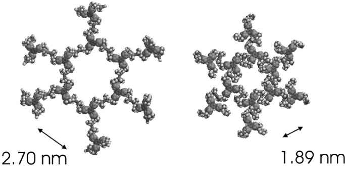
Fig. 8 shows the central hexagon in two optimized geometries of a patch of seven hexagons in the grid, with benzene rings at the vertices and single mercury cations midway between vertex pairs. The searches were started at two likely possibilities with sixfold symmetry, with the S-Hg-S line roughly perpendicular or roughly parallel to the edge of a planar hexagon. After unconstrained optimization, the structure was nearly planar and almost sixfold symmetric. The edge lengths in the two structures were 2.7 and 1.89 nm. From A = (3^3/2/4)r², where A is the area per connector molecule and r is the edge length, these values correspond to 9.47 and 4.64 nm², respectively. The area per redox center is 3.16 and 1.55 nm², respectively, and the surface concentrations Γ are 5.3 × 10⁻¹¹ and 1.1 × 10⁻¹⁰ mol⋅cm⁻² in the grids composed of the large and the small hexagons, respectively.

Figure 8.

Two AM1-optimized structures of the proposed hexagonal network (bound through Hg²⁺ cations).

The modeling is clearly only approximate. The presence of counterions and of the mercury surface has been ignored, the mercury ions have been arbitrarily assumed to be monomeric (Hg⁺ or Hg²⁺ as opposed to Hg), and the AM1 model itself is only approximate. For instance, for the distance from the center of the benzene ring to the distal carbon atom of the carborane cage, it yields 0.66 nm, whereas the x-ray structure yields 0.62 nm (L.P., N.V., Z. Janoušek, B. Grüner, B. Wang, J. Pecka, R. M. Harrison, B. C. Noll, T.F.M., and J.M., unpublished results).

Discussion

The Electrochemical Langmuir Trough.

Langmuir troughs working with the mercury–air interface were first described a third of a century ago (34, 35). The use of a mercury–conducting solvent interface at a well-defined electrochemical potential is appealing for electrochemical studies of layers adsorbed on mercury, but carries its own set of difficulties. The need for a large mercury surface area makes it difficult to satisfy the standard electrochemical requirement that the working electrode be much smaller than the counterelectrode, and the instrument described presently does not permit reliable electrochemical measurements such as cyclic voltammetry, constant-potential coulometry, and impedance determination in which the mercury pool would act as the working electrode. We paid considerable attention to assuring that the counterelectrode was distributed evenly above the mercury in the trough to equalize the iR drop over the whole surface; when this is not done, the mercury surface is unstable and in visible oscillatory motion.

Because the presently described first-generation electrochemical Langmuir trough is used strictly for compression isotherm measurement, we feel that the advantage of simplicity offered by the use of amalgamated copper as a mercury-wetting barrier outweighs the disadvantage represented by the presence of small amounts of copper contaminant in the mercury. The agreement of results, such as the range of metastability, between the Langmuir trough and a pure mercury electrode indicates strongly that copper ions indeed play little or no role in the observed phenomena, and this is assumed in the discussion below. Nevertheless, the shortcomings of the present design are obvious, and based on the experience acquired with the present apparatus, a second-generation instrument that will permit a simultaneous collection of compression isotherms, grazing incidence spectra, and reliable electrochemical data using pure mercury is required.

The Nature of the Adsorbed Layer of 1.

Taken together, the three types of data, cyclic voltammograms, Langmuir compression isotherms, and capacitance curves, agree unambiguously that 1 can interact with the mercury–acetonitrile/LiClO₄ interface in one of three ways. If the potential on the mercury electrode is more negative than ∼ −0.85 V, there is no detectable absorption. If it lies between ∼0 V and ∼ −0.85 V, 1 is physisorbed. If it is positive, 1 induces anodic dissolution of mercury and relatively slowly forms a firmly adsorbed surface layer containing mercury cations, presumably by ligation of the initially present physisorbed 1. Finally, once formed, the firmly adsorbed layer is metastable down to ∼ −0.85 V, even after the mercury cations have been reduced in a fast faradaic process centered near −0.1 V (Fig. 3). Although capacitance measurements for the 12-vertex carborane analogue studied earlier (30) are only available on a dropping mercury electrode, it appears quite clear that the adsorption properties of the two species are virtually identical, as would be expected.

Our primary interest is the structure of the chemisorbed layer of 1, and we have made no attempt to determine the physisorption isotherm by a study of concentration dependence. If the structure indeed is a regular hexagonal grid, as proposed earlier (30) for the 12-vertex carborane analogue, an important milestone in our overall project (1) will have been reached. We believe that the data obtained presently by using the electrochemical Langmuir trough represent a significant step forward compared with the earlier purely electrochemical evidence (30). However, we recognize that an ultimate structure proof will only be provided by a direct tool, such as scanning microscopy or a diffraction method.

The present results are restricted to the mercury–acetonitrile/LiClO₄ interface, but offer an independent determination of the surface area per connector molecule. Under the conditions of the Langmuir isotherm measurement, where we can be sure that only a monolayer is formed and there is no 1 in the bulk supernatant solution, this surface area is ∼6.20 nm² and corresponds to a hexagon edge of 2.18 nm. This measurement is compatible with the smaller of the two hexagon sizes obtained independently from molecular modeling, which offer a choice of 1.89 and 2.70 nm (others may be possible). The difference between 1.89 and 2.18 nm can be attributed to inadequacies in the modeling and to imperfections in the grid, because grain boundaries in the adsorbed monolayer and similar defects will reduce the surface concentration of 1 and thus exaggerate the apparent size of the hexagon. This result permits us to state that the surface area per molecule of 1 is compatible with a hexagonal grid structure.

The area per redox center, and thus the charge on the mercury cations in the grid, remains difficult to determine. The surface concentration of the redox centers deduced from the integrated voltammetric peak areas depends strongly on the potential at which the adsorbed layer was accumulated. The peak value, n_HgΓ_max = 1.14 × 10⁻¹⁰ mol⋅cm⁻², is reached only at +0.2 V. It is the same as found for the 12-vertex carborane analogue (30). The concentration and time dependence of electrode capacitance show that at most potentials, the measured surface concentration is limited kinetically by the slow rate of formation of the organized surface layer. Presumably, at potentials more negative than 0.2 V, the value drops because the rate of oxidative formation of mercury cations at the electrode decreases, and at more positive potentials, it drops because the concentration of 1 physisorbed at the electrode decreases. The value of n_HgΓ_max at 0.2 V does not reach a plateau, and it, too, may be dictated by kinetics and not by surface area requirements.

If we accept the highest observed value, n_HgΓ_max = 1.14 × 10⁻¹⁰ mol⋅cm⁻², the area per mercury ion is 1.47 nm² if n_Hg = 1 (n = 1.5) and 2.94 nm² if n_Hg = 2 (n = 3). Thus, the area per molecule of 1 is 2.21 or 4.41 nm², respectively. The latter measurement agrees closely with the result of AM1 simulation, 4.64 nm², suggesting that n_Hg = 2 is correct and that the binding cations are Hg²⁺ or Hg. It is a priori more likely that anodic oxidation of mercury first produces ions in the familiar dimeric +1 oxidation state, and we currently favor a hexagon edge structure with Hg, such as shown in Fig. 9.

Figure 9.

Most probable structure of a hexagon edge in the proposed hexagonal network of 1 (bound through Hg₂²⁺ cations).

Even the 4.41 nm² value, however, is much smaller than the 6.20 nm² deduced from the Langmuir isotherms by extrapolation to zero pressure, and the difference lies outside the experimental errors of the two measurements. If the highest observed value of n_HgΓ_max is kinetically limited, the electrochemically determined area per molecule is even smaller, and the disagreement with the Langmuir measurements even larger. It is likely that the discrepancy is due the presence of excess 1 in the bulk solution during the electrochemical measurement. Perhaps the Langmuir extrapolation should not be to zero but to some finite pressure. The availability of excess 1 in the supernatant solution could result in more regular and denser packing with fewer bare areas on the mercury surface, and could also induce additional adsorption into the central holes in the hexagons (Fig. 8). However, because the metastability range observed in the two kinds of experiments is exactly the same, we are inclined to believe that the adlayer structures are basically the same. Clearly, a truly reliable determination of the charge state of the mercury cation requires electrochemical measurements in the absence of 1 in bulk solution, i.e., under the conditions encountered in the Langmuir trough. This finding provides a strong motivation for the development of a second-generation electrochemical Langmuir trough mentioned above.

The origin of the huge hysteresis associated with the long-lived metastability of the adsorbed monolayer after the reduction of the mercury cations to elemental mercury is intriguing. Although complexes of Hg(0) are known to exist (36), it is not easy to accept the notion that neutral mercury atoms might stay in place, continuing to bind the thioether chains together, rather than disappearing into the mercury pool. If the thioether sulfur atoms of the molecules of 1 were to interact individually directly with the mercury surface, it is not obvious why the layer should remain ordered and why it would not form spontaneously from the physisorbed layer at negative potentials. If the metastable layer is mercury-ion-free and has a significantly different structure than the mercury-ion-bound grid, it is strange that the difference has no detectable effect on bilayer capacitance (Fig. 7) nor on the surface area per molecule of 1 (Fig. 5). Indeed, it is remarkable that the mere removal of the mercury ions, and of the possibly associated anions, does not have an observable effect in itself, even if the mercury atoms stay in place.

The hysteresis in the capacitance measurement could be explained by arguing that the surface layer of 1 that has been rid of its mercury cation linkers is slow to dissolve simply because its molecules would have to enter a solution that is already saturated with 1. However, the same metastability is observed in the Langmuir trough experiments in which the supernatant acetonitrile solvent does not contain any 1. Several salts have been reported to have a lower surface than bulk solubility (27), presumably because the structure of an adsorbed monolayer is different from that of the bulk solid, and perhaps we are dealing with a similar situation. After the fast reduction of the mercury cations that bind the connector network, the only lateral forces keeping the grid from dissolving would be of the van der Waals type, unless Li⁺ ions from the supporting electrolyte play the role performed by the mercury cations at more positive potentials.

It is also strange that the height of the anodic wave observed in a second sweep toward positive potentials is again limited by the rate of diffusion of 1 to the electrode, as if the thioether sulfur atoms already present in the metastable layer were somehow deactivated. This deactivation would be particularly strange if neutral mercury atoms stayed in place after the reduction. Additional investigations using other solvents and supporting electrolytes are required.

In summary, the present results are encouraging in that they support the proposed hexagonal grid structure of the monolayer formed by 1 on the mercury/LiClO₄ interface at positive potentials, but they still leave important issues open. Salient among these are a direct grid structure proof, the structure of the mercury cations in the grid, and the nature of the electrochemical hysteresis.

References

- 1.Michl J, Magnera T F. Proc Natl Acad Sci USA. 2002;99:4788–4792. doi: 10.1073/pnas.052016299. [DOI] [PMC free article] [PubMed] [Google Scholar]
- 2.Heyrovský J, Kůta J. Principles of Polarography. Prague: NCSAV/Academic; 1965. pp. 171–175. [Google Scholar]
- 3.Armstrong R D, Fleischmann M. Z Phys Chem N F. 1967;52:131–143. [Google Scholar]
- 4.Müller C, Claret J, Sarret M. J Electroanal Chem. 1986;207:263–278. [Google Scholar]
- 5.Andreoli R, Battistuzzi Gavioli G, Benedetti L, Borsari M, Fontanesi C. J Electroanal Chem. 1990;293:209–218. [Google Scholar]
- 6.Kolthoff I M, Miller C S. J Am Chem Soc. 1941;63:1405–1411. [Google Scholar]
- 7.Zuman P. Coll Czech Chem Commun. 1955;20:649–661. [Google Scholar]
- 8.Br̆ezina M, Zuman P. Polarography in Medicine, Biochemistry and Pharmacy. New York: Academic; 1958. pp. 470–513. [Google Scholar]
- 9.Armstrong R D, Porter D F, Thirsk H R. J Phys Chem. 1968;72:2300–2306. [Google Scholar]
- 10.Peter L M, Reid J D, Scharifker B R. J Electroanal Chem. 1981;119:73–91. [Google Scholar]
- 11.Benucci C, Scharifker B R. J Electroanal Chem. 1985;190:199–212. [Google Scholar]
- 12.Slowinski K, Chamberlain R V, Miller C J, Majda M. J Am Chem Soc. 1997;119:11910–11919. [Google Scholar]
- 13.Muskal N, Mandler D. Electrochim Acta. 1999;45:537–548. [Google Scholar]
- 14.Calvente J J, Andreu R, Gil M-L A, González L, Alcudia A, Domínguez M. J Electroanal Chem. 2000;482:18–31. [Google Scholar]
- 15.Tadini Buoninsegni F, Becucci L, Moncelli M R, Guidelli R. J Electroanal Chem. 2001;500:395–407. [Google Scholar]
- 16.Zuman P, Rusling J F. In: Encyclopedia of Colloid and Surface Science. Hubbard A T, editor. Vol. 3. New York: Marcel Dekker; 2002. pp. 4143–4164. [Google Scholar]
- 17.De Levie R. In: Advances in Electrochemistry and Electrochemical Engineering. Gerischer H, Tobias C, editors. Vol. 13. New York: Wiley; 1984. pp. 1–67. [Google Scholar]
- 18.Buess-Herman C. J Electroanal Chem. 1985;186:27–39. [Google Scholar]
- 19.Sridharan R, de Levie R. J Electroanal Chem. 1986;201:133–143. [Google Scholar]
- 20.Benedetti L, Borsari M, Battistuzzi Gavioli G, Fontanesi C. J Electroanal Chem. 1990;279:321–330. [Google Scholar]
- 21.Guerrieri A, Cataldi T R I, Palmisano F, Zambonin P G. J Electroanal Chem. 1991;314:117–134. [Google Scholar]
- 22.Philipp R, Retter U. Electrochim Acta. 1995;40:1581–1585. [Google Scholar]
- 23.Retter U, Kant W. Thin Solid Films. 1995;256:89–93. [Google Scholar]
- 24.Millán J I, Amaro R R, Ruiz J J, Camacho L. J Phys Chem B. 1999;103:3669–3676. [Google Scholar]
- 25.Bewick A, Fleischmann M, Thirsk H. Trans Faraday Soc. 1962;58:2200–2216. [Google Scholar]
- 26.Philipp R, Retter U. Thin Solid Films. 1995;259:59–64. [Google Scholar]
- 27.Elliott C M, Murray R W. J Am Chem Soc. 1974;96:3321–3322. [Google Scholar]
- 28.Elliott C M, Murray R W. Anal Chem. 1976;48:259–267. [Google Scholar]
- 29.Budevski E, Staikov G, Lorenz W J. Electrochim Acta. 2000;45:2559–2574. [Google Scholar]
- 30.Pospíšil L, Heyrovskı M, Pecka J, Michl J. Langmuir. 1997;13:6294–6301. [Google Scholar]
- 31.Dewar M J S, Zoebisch E G, Healy E F, Stewart J J P. J Am Chem Soc. 1985;107:3902–3909. [Google Scholar]
- 32.Pospíšil L, Fiedler J, Fanelli N. Rev Sci Instrum. 2000;71:1804–1810. [Google Scholar]
- 33.Bard A J, Faulkner R L. Electrochemical Methods, Fundamentals and Applications. New York: Wiley; 2001. , Ch. 13, pp. 534–579. [Google Scholar]
- 34.Smith T. J Coll Interface Sci. 1967;26:509–517. [Google Scholar]
- 35.Smith T. Advan Coll Interface Sci. 1972;3:161–221. [Google Scholar]
- 36. Catalano, V. J., Malwitz, M. A. & Noll, B. C. (2001) Chem. Commun., 581–582.