Transience of Coastal Water Table Rise in Response to Sea‐Level Rise

Abstract

Coastal shallow groundwater is susceptible to adverse sea‐level rise (SLR) impacts. Existing research primarily focuses on SLR‐induced salinization of coastal aquifers. There is limited understanding of the magnitudes and rates of water table rise in response to SLR, which could lead to groundwater flooding and associated infrastructure challenges. This study used a variable‐density groundwater flow model to quantify the transient movement of the water table in response to various SLR scenarios and rates, considering a range of aquifer parameters for both fixed‐head and fixed‐flux inland boundary conditions. The SLR scenario based on realistic and progressive SLR projections resulted in a smaller water table rise than the instantaneous or gradual SLR scenarios at 100 years, despite a final identical SLR. Rates of water table rise were always less than SLR, decreased with distance from the coastline, and were proportional to SLR. The magnitude and rate of water table rise in response to SLR were largest for fixed‐flux conditions. It also took longer for the rate of water table rise to equilibrate after the commencement of SLR for fixed‐flux conditions than for fixed‐head conditions. As such, fixed‐flux conditions represent a greater hazard for water table rise, and the maximum impact may not be experienced for decades. This delayed response poses challenges to planners and managers of coastal groundwater systems. Introducing a drain reduced water table rise more on the inland side of the drain than on the coastal side. Subsurface infrastructure may limit SLR impacts, but further effects need to be carefully considered.

Introduction

Almost 11% of the world's population lives within the low‐elevation coastal zone, areas that are hydrologically connected to the sea and less than 10 m above sea level (McGranahan et al. ²⁰⁰⁷; IPCC ²⁰²²; Magnan et al. ²⁰²²). Sea‐level rise (SLR) caused by climate change will adversely impact coastal areas globally (Church and White 2011; Cazenave and Cozannet ²⁰¹⁴; Oppenheimer et al. ²⁰¹⁹). In response to SLR, changes occur in coastal shallow groundwater, such as saltwater intrusion and groundwater rise (Masterson and Garabedian 2007; Rotzoll and Fletcher ²⁰¹³; Befus et al. ²⁰²⁰; Bosserelle et al. ²⁰²²; Morgan ²⁰²⁴). Saltwater intrusion is the landward encroachment of saline water into fresh coastal aquifers (Werner and Simmons 2009). The main impact of saltwater intrusion is the salinization of fresh groundwater, leading to a reduction in water security and the degradation of ecosystems (Morgan et al. 2012; Herbert et al. ²⁰¹⁵). Groundwater rise is the upward movement of the water table due to the long‐term increase of the mean sea level and extreme levels (Bosserelle et al. 2022); hereafter, the term water table rise is used. The impacts of water table rise include damage to (1) underground pipelines such as stormwater, water supply, and sewage systems, that is, inflow and infiltration; (2) basements, building foundations, and drainage, that is, flooding and structural instability; (3) roads, surface structures, and networks, that is, flooding and erosion; (4) ecosystems in coastal rivers, drains, creeks, streams, and wetlands, that is, saline intrusion and habitat loss (Rotzoll and Fletcher 2013; May ²⁰²⁰; Magnan et al. ²⁰²²). The principal coastal implication due to SLR and water table rise is flooding (Habel et al. 2023). Consequently, the changes in coastal shallow groundwater can directly increase the exposure to flooding hazards in the coastal zone (Cazenave and Cozannet 2014; Rahimi et al. ²⁰²⁰; IPCC ²⁰²²). While numerical modeling of surface hydrodynamics is widely used to assess the impact of SLR‐induced coastal flooding, little is known about the contribution of shallow groundwater to flooding (Passeri et al. 2015).

The impact of SLR on coastal shallow groundwater was first assessed by Barlow (2003), then Masterson and Garabedian (2007) and specifically considered groundwater rise. A series of groundwater modeling articles followed, including the assessment of the saltwater intrusion problem under SLR by Werner and Simmons (2009). Numerous subsequent studies have mainly focused on saltwater intrusion and salinization impacts (Chang et al. 2011; Ataie‐Ashtiani et al. ²⁰¹³; Lu and Werner ²⁰¹³; Rasmussen et al. ²⁰¹³; Morgan et al. ²⁰¹⁵; Ketabchi et al. ²⁰¹⁶; Mehdizadeh et al. ²⁰¹⁷; Guo et al. ²⁰²⁰). Many studies have explored susceptibility and vulnerability to SLR by estimating changes in the steady‐state saltwater/freshwater interface position with SLR for different combinations of hydrogeologic parameters and inland boundary conditions (Werner et al. 2012; Morgan et al. ^2013b; Shi et al. ²⁰¹⁸; Shi et al. ²⁰²⁰; Luo et al. ²⁰²²). Both analytic (Strack 1976) and numerical (Morgan et al. ^2013a; Sun et al. ²⁰¹⁷; Zamrsky et al. ²⁰²⁴) modeling approaches have been applied.

While steady‐state analyses help estimate the final interface (or long‐term) position for a new sea level, they do not assess the transience of interface movement in response to SLR nor the timescales of interface movement. Here, timescales refer to the time required for the interface to reach equilibrium with the new sea level (i.e., no significant change in interface position from 1 year to the next). Watson et al. (2010) explored the transience of saltwater intrusion in typical unconfined coastal aquifer settings and, along with subsequent studies, found timescales in the order of 100 years (Lu and Werner 2013; Morgan et al. ²⁰¹⁵; Ketabchi et al. ²⁰¹⁶; Ranjbar et al. ²⁰²⁰). Additionally, transient analyses identified the saltwater intrusion overshoot phenomenon, where the interface temporarily extends further inland than the long‐term steady‐state post‐SLR position (Watson et al. 2010; Morgan et al. ²⁰¹⁵). This phenomenon highlights a need for transient analyses because, contrary to previous assumptions, a steady‐state model may not represent a worst case in terms of salinization from SLR.

Relative to the numerous studies on SLR and saltwater intrusion, few studies have assessed the impact of SLR on coastal groundwater levels. The study by McCobb and Weiskel (2003) and Masterson (2004) used data‐analysis techniques on hydrographs of groundwater levels from a long‐term monitoring program (1950 to 2002) at Cape Cod (Massachusetts, USA) and found that long‐term increasing trends in observed groundwater levels matched the measured rate of SLR at the Boston tide gauge (McCobb and Weiskel ²⁰⁰³; Masterson ²⁰⁰⁴). Similarly, and more recently, Smith and Medeiros (2019) used a data‐driven approach to study historical records of groundwater levels (2000 to 2017) from the Cape Cod peninsula and showed that SLR may be partly responsible for the increasing long‐term water table trends. Additionally, Smith and Medeiros (2019) demonstrated that groundwater levels at monitoring sites near the coastline were more responsive to the mean sea level increase than inland sites, at a distance of 4 km from the coastline. These studies, focusing on coastal aquifers along the Atlantic coast of the United States, support the hypothesis that groundwater levels will rise with SLR.

Previous studies have looked at the response of groundwater levels to SLR using steady‐state analytic models (Morgan and Werner 2016; Morgan ²⁰²⁴). Steady‐state numerical modeling approaches were predominantly used to quantify the magnitude of water table rise (Bjerklie et al. 2012; Walter et al. ²⁰¹⁶; Habel et al. ²⁰¹⁷; Sukop et al. ²⁰¹⁸; Knott et al. ²⁰¹⁹; Yu et al. ²⁰²²). Bjerklie et al. (2012) and Walter et al. (2016) found increasing groundwater levels using numerical models of the coastal city of New Haven (Connecticut, USA) and Cape Cod (Massachusetts, USA), respectively. Both studies found that the increase in the elevation of groundwater tables resulting from SLR varied with the distance from the coastline and was dependent on surface water features (e.g., stream, tidal river, and estuary).

The rise of the water table triggering groundwater flooding has recently received more attention related to SLR‐induced flooding hazards in unconfined coastal aquifers. Steady‐state numerical simulations have been used to predict where groundwater flooding will occur in response to SLR. Simulations included different coastal settings considering unique geological and hydrological characteristics (i.e., beach and estuarine environments, heavily developed and hardened shorelines) and showed where higher water tables will increase vulnerability to coastal flooding in New Hampshire (Knott et al. 2019), California (Hoover et al. 2017; Befus et al. ²⁰²⁰), Florida (Sukop et al. 2018), and Hawaii (Habel et al. 2019; Habel et al. ²⁰²⁰). The criteria used to define vulnerability to coastal flooding related to rising water tables included the magnitude of groundwater rise and its inland extent, the depth of the water table, the proximity to tidal water bodies, and the topography. Befus et al. (2020) showed that coastal groundwater shoaling and emergence vulnerability in California would increase where high water tables were observed, especially in regions of low‐lying topography. Their study used a sharp interface steady‐state analyses at a large regional scale to predict the land area sensitive to SLR‐induced water table flooding for different inland boundary conditions and hydrogeological parameters.

A few studies have highlighted the importance of understanding and evaluating the transient water table response to SLR (Rotzoll and Fletcher 2013; Walter et al. ²⁰¹⁶; Befus et al. ²⁰²⁰). A notable study by Masterson and Garabedian (2007) has simulated transient water table rise in response to SLR, which used a generic model broadly representative of the Cape Cod freshwater lens systems. In that study, it was found that groundwater levels increased in response to SLR, as did streamflow, and the discharge into the stream prevented the water table from rising above the stream bed level (Masterson and Garabedian 2007). The simulated rates of water table rise (defined as the measure of groundwater level change within a fixed period) were lower than the SLR rate. The rise and the rates were highest at the site closest to the coastline and the site farthest from the stream. While the study of Masterson and Garabedian (2007) considered a freshwater lens system (i.e., a strip island lens setting—as detailed in Morgan and Werner ²⁰¹⁴), there has been no assessment to date of the transient water table response to SLR in continental unconfined coastal aquifers, nor the influence of aquifer parameters and boundary conditions.

Damage to roads, subsurface pipes, essential services access, evacuation routes, landfills, and ground conditions may be expected as groundwater levels rise with SLR (Walter et al. 2016; Knott et al. ²⁰¹⁷; Hummel et al. ²⁰¹⁸) and increased natural hazards susceptibility such as liquefaction and flooding (Burke‐Flask et al. ²⁰²¹; Grant et al. ²⁰²¹). Globally, there needs to be more knowledge of the variability of the impacts of SLR on coastal groundwater and infrastructure systems over time, but limited research has been carried out to date. Su et al. (2020) used numerical modeling to show that in areas where wastewater and stormwater pipes are not leaky (i.e., fully repaired), groundwater levels are elevated relative to other areas, potentially causing groundwater infiltration and flooding problems into other infrastructure. Su et al. (2022) further found that tides and SLR will exacerbate the risk of flooding in coastal urban areas due to the interaction between groundwater and infrastructure (Su et al. 2022). Clearly, understanding the transience of rising groundwater levels in response to SLR through modeling is critical to managing infrastructure systems in cities and settlements along the coastline.

This study aims to improve understanding of the transience of water table rise in response to SLR for various SLR scenarios, hydrogeological conditions, and inland boundary conditions. A variable‐density numerical modeling approach is used to quantify the magnitude and rate of the rise in the water table for an unconfined continental coastal aquifer setting. Additionally, the time for the water table to stop rising following the cessation of SLR is assessed (i.e., the timescale of water table rise). The time for rates of water table rise to equilibrate following the commencement of SLR is quantified, which is referred to as the response time. This study also investigates the presence and impact of subsurface drainage infrastructure on water table rise. The specific objectives of this study are to quantify the changes in water table elevation and the rates of water table rise for various SLR scenarios and assess the impact of: (1) rates of SLR (i.e., instantaneous, linear and non‐linear); (2) various hydraulic parameters (i.e., changes in hydraulic diffusivity); and (3) subsurface drainage infrastructure.

Methods

Conceptual Model

The conceptual model used in this study is an idealized representation of a homogeneous unconfined continental coastal aquifer (Figure 1). The hypothetical cross‐section extends from the coastline to an inland boundary and includes the saltwater‐freshwater interface or the transition zone (Figure 1a). This study's cross‐section diagram and model section included a simplified but realistic topographic feature (i.e., an area above mean sea level [MSL]). This serves to ensure that there is a thick upper layer in the numerical model where water table fluctuations, in response to changes in sea level, do not result in emergence of the water table above land surface. Using a simplified land surface in modeling studies is common, and coastal topographic features only substantially impact groundwater processes when coupling surface‐subsurface models to simulate ocean flooding (Yu et al. 2016). This simplification improves computational efficiency and focuses on relative changes in groundwater dynamics due to SLR, avoiding unnecessary complexity from surface details that minimally impact subsurface processes. The offshore boundary is the depth to the aquifer base measured from MSL z ₀ [L] (Figure 1a). The hydraulic head h _f [L] relative to MSL at a distance x [L] from the coastline and the depth to the saltwater‐freshwater interface z [L] is given by the Ghyben‐Herzberg relation (Ghyben 1889; Herzberg ¹⁹⁰¹), $z=h_f/\delta$, where δ is the dimensionless density ratio $\delta =\left({\rho }_s-{\rho }_f\right)/{\rho }_f$, and ρ _f and ρ _s are fresh water and saltwater densities [M/L³], 1000 and 1025 kg/m³, respectively.

Figure 1.

Schematic showing (a) the conceptual model and variables of the unconfined coastal aquifer and (b) corresponding numerical model domain, including the observation locations.

A constant and uniform net recharge W [L/T] is spatially distributed over the land from the coastline and accounts for infiltration, evapotranspiration, and distributed pumping. Fluxes include freshwater discharge to the sea q ₀ [L²/T] and the lateral flow q _b [L²/T] from aquifers inland of the landward boundary at a distance x _b [L] and for an inland head h _b [L] (Figure 1a). Aquifer parameters are hydraulic conductivity K [L/T] and specific yield S _y [−].

Conceptually, two types of coastal groundwater systems can apply, and many saltwater intrusion modeling studies have simulated these using two different inland boundary conditions (Sun et al. 2017). The coastal water table can either be (1) head or topography‐controlled (or limited), where the water table elevation is closely associated with topography, hereafter referred to as fixed‐head conditions, or (2) recharge or flux‐controlled water tables, where the water table is disconnected from topography, hereafter referred to as fixed‐flux conditions (Gleeson et al. 2011; Michael et al. ²⁰¹³). It is widely recognized that these two inland boundary conditions (i.e., fixed‐head or fixed‐flux) represent end members in regard to the responses of the water table and interface to SLR for steady‐state conditions. Maximum saltwater intrusion and minimum water table rise are observed for fixed‐head conditions, while minimum saltwater intrusion and maximum water table rise are observed for fixed‐flux conditions (Werner and Simmons 2009; Morgan et al. ²⁰¹⁵; Morgan ²⁰²⁴).

Numerical Model

The analysis of coastal groundwater systems using numerical models is a common approach for simulating future projections and carrying out analyses (Jiao and Post 2019). In this study, SEAWAT (Guo and Langevin 2002; Langevin et al. ²⁰⁰⁸) was used for steady‐state and transient modeling of the water table response to SLR. SEAWAT couples MODFLOW and MT3DMS to simulate variable‐density groundwater flow and solute transport, and has been verified and widely used for simulating coastal groundwater systems and saltwater intrusion (Chang et al. 2011; Webb and Howard ²⁰¹¹; Lu and Werner ²⁰¹³; Badaruddin et al. ²⁰¹⁷; Post et al. ²⁰¹⁸; Ranjbar et al. ²⁰²⁰). The variable‐density groundwater flow equations are solved by formulating the equivalent freshwater head as the principal dependent variable. Although the governing equations of SEAWAT are not provided here, the specific numerical methods and equations used in SEAWAT are described in Guo and Langevin (2002) and Langevin et al. (2008).

The model was a section of 5000 m long, as shown in Figure 1b, extending 300 m offshore from the coastline. The grid comprised of 1 row, that is 10 m by 25 m spacing, discretised in 200 columns and 30 layers (from −1 m MSL to −30 m). The grid selection was tested by changing the length of the section and spacing until the best computational time and the minimal discrepancy of the results between the analytical and numerical models was achieved. The discretization of the model grid was consistent with a Peclet number, Pe [−] less than 1, as recommended by Voss and Souza (1987) to reduce numerical instabilities: $\mathit{Pe}=∆l/4{\alpha }_L$, where Δl [L] was the size of the local distance between sides of a cell measured along the local flow direction and α _L [L] is the total longitudinal dispersion coefficient. Longitudinal dispersivity was set at 10 m and the transverse dispersivity was set at 1 m in the numerical model. The depth to the aquifer base measured from MSL, z ₀ [L] is 30 m. The top model layer elevation varied from 0 m at the saltwater (ocean) boundary to 7.5 m rise along the coastal system (e.g., coastal barrier, dunes) and then flattened to 4 m above 0 m MSL. The inland distance from the coastline, x _b [L] was 4700 m. The initial aquifer parameters were horizontal hydraulic conductivity K _x [L/T] of 10 m/d equal to vertical hydraulic conductivity K _z [L/T], effective porosity n [−] of 0.3 and specific yield S _y [−] of 0.2. Homogeneous and isotropic conditions are assumed.

Cells representing the ocean (saltwater boundary) were assigned specified head boundary conditions. Saltwater enters the groundwater system, and freshwater exits through a leaky layer at the sloping boundary of the model using a horizontal approximation and then becomes vertical. A saltwater head equal to the initial MSL (coastline head) at 0 m and a fixed saltwater concentration of 35 ppt or kg/m³ (i.e., average salinity of seawater as used by Webb and Howard ²⁰¹¹) were assigned to all the specified head cells. Cells in the topmost layer of the model were assigned a low specified flux W [L/T] of 3 × 10⁻⁵ m/day from a hypothetical net recharge rate of a coastal system (Chang et al. 2011). To account for both a fixed‐head and fixed‐flux coastal groundwater system classification, two inland boundary conditions were used. The fixed‐head condition was applied using a specified head at the inland boundary h _b [L] of 3 m. The fixed‐flux condition was applied using a specified flux at the inland boundary (with the flux equal to that occurring for the fixed‐head condition) and uniformly distributed from the top to bottom layers. As such, the head and flux (whether assigned or calculated) at the inland boundary are the same for both the fixed‐head and fixed‐flux conditions. No flow was applied at the bottom of the model, and the initial background concentration was 0 kg/m³.

Steady‐State Modeling

Pre‐SLR steady‐state simulations were carried out for fixed‐head and fixed‐flux inland boundary conditions. The simulations were run for 10,000 years, and steady‐state conditions were reached (i.e., no change in head or salinity). The coastal boundary head was set to 0 m MSL, and the simulation started with a freshwater‐filled aquifer. Using initial aquifer geometry and parameters, the pre‐SLR steady‐state simulations were carried out, and the results were used as initial conditions for the head and salinity distribution for the post‐SLR steady‐state simulations.

Post‐SLR steady‐state simulations used a SLR of 1 m, implemented by assigning a coastal boundary head of 1 m MSL. The model was run for a period of 200 years, and a new post‐SLR steady‐state condition was reached at the end of the simulation.

The numerical model was also validated by comparing results from the post‐SLR steady‐state simulation to those obtained analytically using the Strack (1976, 1989) sharp‐interface solution. Specifically, the change in water table elevation was compared. The change in water table elevation is defined as the SLR‐induced change in water table height Δh [L] relative to the base of the aquifer (Morgan and Werner 2016; Bosserelle et al. ²⁰²²):

$$∆h=h{\prime }_f-h_f+∆z$$ (1)

where h _f [L] is hydraulic head as a function of distance from the coast, and h' _f is the new water table elevation for SLR of ∆z [L]. For each type of inland boundary condition, the Pearson correlation coefficient (r) between estimated $∆h$ (numerical and analytic model) was used to assess the validity of the model. The comparison was carried out for both fixed‐head and fixed‐flux inland boundary conditions using a python code for the analytic modeling.

The saltwater/freshwater interface location in the post‐SLR numerical model was also compared to the analytic solution. The interface location is characterized by the distance from the coastline to the intersection of the interface and aquifer base x _T [L]. In the numerical model, the interface between fresh and saline groundwater is dispersive, and the 50% isochlor, where the salt concentration is 17.5 kg/m³ in the aquifer bed, was used to represent the interface location. Pool and Carrera (2011) and later Lu and Werner (2013) proposed an empirical correction factor to make analytical non‐dispersive solutions more consistent with variable density dispersive numerical models. In this study, the values of x _T post‐SLR were calculated with the correction factor from Lu and Werner (2013).

Transient Modeling

Transient simulations were carried out to assess (1) the timescales and rates of the water table rise and the response times for both fixed‐head and fixed‐flux inland boundary conditions, (2) the influence of rates of SLR and aquifer parameters on water table elevation, and (3) the effects of subsurface infrastructure acting as drains. Table 1 outlines the scenarios and provides a summary (i.e., reference guide) for the approach described in the numerical modeling section. The change in modeled heads in the top layer (i.e., at the water table) was used to calculate a transient value of ∆h, referred to as ∆h _t [L] and the rate of water table rise, ν [L/T] is calculated using ∆h _t over a yearly time period. The rate of SLR is generally expressed as a trend in millimeters per year, mm/year (Church and White 2011; Cazenave and Cozannet ²⁰¹⁴), and ν has a comparable unit.

Table 1.

Reference Guide of Modeling Scenarios.

Case	Simulation	Approach
Base case	Pre‐SLR steady‐state	For fixed‐head and fixed‐flux inland boundary conditions No SLR
	Post‐SLR steady‐state	Initial conditions for head and salinity distribution from the pre‐SLR steady‐state For fixed‐head and fixed‐flux inland boundary conditions SLR of 1 m
Scenario 1	Post‐SLR transient	Based the Base Case settings Initial conditions for head and salinity distribution from the pre‐SLR steady‐state For fixed‐head and fixed‐flux inland boundary conditions Instantaneous SLR of 1 m
Scenario 2	Post‐SLR transient	Based the Base Case settings Initial conditions for head and salinity distribution from the pre‐SLR steady‐state For fixed‐head and fixed‐flux inland boundary conditions Gradual linear SLR of 1 m over 100 years (i.e., 10 mm/year)
Gradual linear SLR	Post‐SLR transient (3 models)	Based on Scenario 2 For fixed‐head and fixed‐flux inland boundary conditions Gradual linear SLR of 0.4, 0.8 and 1.6 m (i.e., 4, 8, and 16 mm/year)
Change in hydraulic diffusivity	Post‐SLR transient (4 models)	Based on Scenario 2 For fixed‐head and fixed‐flux inland boundary conditions D values of 15, 150, 1000, and 3000 m2/d
Testing Anisotropy	Post‐SLR transient (2 models)	Based on Scenario 2 For fixed‐head and fixed‐flux inland boundary conditions K z /K x 0.1 and K z /K x 0.01
Subsurface infrastructure	Post‐SLR transient	Based on Scenario 2 For fixed‐head and fixed‐flux inland boundary conditions Drain boundary condition
Scenario 3	Post‐SLR transient	Based the base case settings Initial conditions for head and salinity distribution from the pre‐SLR steady‐state For fixed‐head and fixed‐flux inland boundary conditions Non‐linear SLR over 100 years (i.e., from 7 to 16 mm/year)

The Base Case described the set of initial parameters and model settings discussed in the numerical modeling section. The Base Case simulates pre‐SLR and post‐SLR conditions for both fixed‐head and fixed‐flux inland boundary conditions and is used for comparison with scenarios and sensitivity testing, as described in Table 1.

Sea‐Level Rise Scenarios and Rates of Sea‐Level Rise

Using the Base Case geometry settings and aquifer parameters, three SLR scenarios were simulated. The scenarios are: (1) instantaneous SLR of 1 m; (2) gradual linear SLR of 1 m over 100 years (i.e., 10 mm/year); (3) non‐linear SLR over 100 years (i.e., from 7 to 16 mm/year)– based on realistic projections from scenario SSP2‐4.5, medium confidence projection where SSP is the Shared Socio‐economic Pathway (IPCC ²⁰²¹).

In addition to the gradual linear SLR (Scenario 2) detailed above, three SLR rate simulations were carried out with gradual linear rates of 4, 8, and 16 mm/year. over 100 years – equivalent to a SLR of 0.4, 0.8, and 1.6 m, respectively.

Change in Hydraulic Diffusivity

The impact of hydraulic diffusivity D [L²/T] (i.e., the ratio of transmissivity to storativity) on v was assessed using a gradual linear SLR of 1 m over 100 years (equal to the rate of SLR in Scenario 2). Here, D values of 15, 150, 1000, and 3000 m²/d were applied (D of 1500 m²/d for the Base Case included in results) and are representative of K values ranging between 0.1 and 10 m/d for an aquifer thickness of 30 m, and S _y values ranging between 0.1 and 0.3. These values are broadly typical of coastal aquifers (Chang et al. 2011; Lu and Werner ²⁰¹³; Zamrsky et al. ²⁰²⁰). Post‐SLR transient simulations used the modeled steady‐state head and salinity distribution from the pre‐SLR simulations as initial conditions for each value of D.

Testing Anisotropy

Two anisotropy ratios (K _v /K _h ), that is, 0.1 and 0.01, are introduced to observe the effects of anisotropic coastal aquifers (K _h  > K _v ) on ∆h _t and ν for Scenario 2. Typical anisotropy ratios for modeling studies are within this range of values from 0.1 to 0.05 (Watson et al. 2010; Zamrsky et al. ²⁰²⁴). Pre‐SLR conditions are modeled using these new K _v values, and the modeled steady‐state head and salinity distribution are used in the post‐SLR transient simulations.

Subsurface Infrastructure

The impact of subsurface infrastructure on ∆h _t and v was assessed using a gradual linear SLR of 1 m over 100 years (equal to the rate of SLR in Scenario 2). Initial conditions were taken from the Base Case pre‐SLR steady‐state simulation where the drain (e.g., open or subsoil) was located above the water table elevation. The subsurface drainage infrastructure (representing a stormwater drain, for example) is simulated using a drain boundary condition at a generic location of 1000 m from the coastline and 1.5 m MSL. The drain location is positioned such that it will intercept rising groundwater levels under future SLR and allow observation of the impact of subsurface drainage infrastructure.

Results

Steady‐State Models and Validation

Values of ∆h at various distances from the coastline for the post‐SLR steady‐state numerical model and equivalent analytic model are shown in Table 2. Values are similar (r = 0.997 for fixed‐head inland boundary conditions, and r = 0.986 for fixed‐flux inland boundary condition), although ∆h determined using the numerical modeling is slightly larger than for the analytic modeling. These findings confirm the validity of the numerical model.

Table 2.

Comparison Between ∆h for an Instantaneous SLR of 1 m Using Numerical and Analytic Modeling and Different Inland Boundary Conditions.

Setting	Distance (m)	500	1000	1500	3000	4700
Fixed‐head inland boundary condition	∆h, analytic model (m)	0.895	0.781	0.669	0.348	0
	∆h, numerical model (m)	0.902	0.786	0.673	0.412	0
Fixed‐flux inland boundary condition	∆h, analytic model (m)	0.999	0.989	0.978	0.953	0.934
	∆h, numerical model (m)	1	0.999	0.989	0.967	0.943

Post‐SLR, the value of x _T was 353 m in the numerical model and 401 m from the analytic model, for fixed‐head inland boundary conditions. Conversely, for fixed‐flux inland boundary conditions, x _T was 265 m in the numerical model and 289 m in the analytic model. As such, values of x _T are comparable for numerical and analytic models within the limitations of the grid discretization and mixing processes.

Transient Models

Sea‐Level Rise Scenarios and Rates of Sea‐Level Rise Simulations

Simulated values of ∆h _t for an instantaneous SLR (Scenario 1), for fixed‐head and fixed‐flux inland boundary conditions, are shown in Figure 2. For the fixed‐head inland boundary condition, ∆h _t approaches a maximum value more rapidly (Figure 2a) than for the fixed‐flux inland boundary condition (Figure 2b). This is the case at all distances from the coastline. Additionally, for Scenario 1, a maximum value of ∆h _t is reached more rapidly with decreasing distance from the coastline, for both fixed‐head and fixed‐flux inland boundary conditions. The timescale is longer for fixed‐flux conditions (up to 80 years at the inland boundary) than for fixed‐head conditions (less than 20 years), as shown in Figure 2.

Figure 2.

Numerical model results for the change in groundwater level ∆h _t at different distances from the coastline for SLR Scenario 1 and for (a) fixed‐head inland boundary condition and (b) fixed‐flux inland boundary condition.

Simulated values of ∆h _t for gradual linear SLR (Scenario 2) and gradual non‐linear SLR projection (Scenario 3), for fixed‐head and fixed‐flux inland boundary conditions, are shown in Figure 3. The SLR values (∆z) used within the simulations are shown in Figure 3a. For Scenario 3, the rate of SLR increased from 7 mm/year to 16 mm/year over 100 years.

Figure 3.

(a) SLR values (∆z) for Scenario 2 (shaded) and Scenario 3 (dashed); and numerical model results for the change in groundwater level ∆h _t at different distances from the coastline in response to those SLR scenarios for (b) fixed‐head and (c) fixed‐flux inland boundary conditions.

Figure 3 indicates that the simulated trend in ∆h _t broadly followed the SLR trend. For Scenario 2, the trend in ∆h _t was linear and gradual. For Scenario 3, the trend in ∆h _t was non‐linear and accelerated at later times. As such, the value of ∆h _t was larger for Scenario 2 than for Scenario 3 at all times.

Values of ∆h _t at various distances from the coastline after 100 years are summarized in Table 3 for Scenarios 1, 2, and 3. At all distances from the coast, ∆h _t values are largest for Scenario 1 and fixed‐flux inland boundary conditions. Conversely, at all distances from the coast, ∆h _t values are smallest for Scenario 3 and fixed‐head inland boundary conditions.

Table 3.

Simulated Change in Groundwater Levels ∆h _t After 100 Years of SLR at Different Distances from the Coastline in Response to SLR (Scenarios 1, 2, and 3) for Fixed‐Head and Fixed‐Flux Inland Boundary Conditions.

Setting	Distance (m)	500	1000	1500	3000	4700
Fixed‐head inland boundary condition	∆h t , Scenario 1 (m)	0.902	0.786	0.673	0.412	0
	∆h t , Scenario 2 (m)	0.890	0.767	0.650	0.390	0
	∆h t , Scenario 3 (m)	0.883	0.757	0.638	0.379	0
Fixed‐flux inland boundary condition	∆h t , Scenario 1 (m)	1	0.999	0.989	0.967	0.943
	∆h t , Scenario 2 (m)	0.972	0.928	0.890	0.821	0.771
	∆h t , Scenario 3 (m)	0.958	0.904	0.858	0.776	0.719

For fixed‐flux inland boundary conditions, the difference between ∆h _t for Scenarios 1 and 2 increases further from the coastline, being the minimum at 500 m from the coastline (i.e., 0.028 m) and reaches the maximum at the inland boundary (i.e., 0.172 m). However, for fixed‐head inland boundary conditions, the difference between ∆h _t for Scenarios 1 and 2 is the minimum at the inland boundary (i.e., 0 m) and the maximum at 1500 m from the coastline (i.e., 0.023 m). Also, the difference between ∆h _t for Scenarios 1 and 2 is larger for fixed‐flux inland boundary conditions at all distances. That is, the impact of the rate of SLR on ∆h _t is greatest when the inland boundary is fixed‐flux.

At 100 years, the value of ∆h _t differed for Scenarios 2 and 3 (Table 3). For fixed‐flux inland boundary conditions, the difference between ∆h _t for Scenarios 2 and 3 increases further from the coastline, being the minimum at 500 m from the coastline (i.e., 0.014 m) and reaching the maximum at the inland boundary (i.e., 0.052 m). However, for fixed‐head inland boundary conditions, the difference between ∆h _t for Scenarios 2 and 3 is the minimum at the inland boundary (i.e., 0 m) and the maximum at 3000 m from the coastline (i.e., 0.012 m). This difference was larger for a fixed‐flux inland boundary condition and also increased with increasing distance from the coastline (Figure 3c). The progressive increase in rates of SLR from 7 mm/year. to 16 mm/year. over 100 years has less impact on ∆h _t than the linear rise in sea level of 10 mm/year. over 100 years.

Using Scenario 2, three SLR rate simulations were carried out with gradual linear rates of 4, 6, and 16 mm/year. over 100 years, in addition to the original 10 mm/year. over 100 years. The results, in terms of v, are presented in (Figure 4a through 4h) for fixed‐head and fixed‐flux inland boundary conditions.

Figure 4.

Simulations results showing rates of water table rise v for Scenario 2 and changes in rates of SLR; 4 mm/year (a) fixed‐head and (b) fixed‐flux inland boundary conditions, 8 mm/year (c) fixed‐head and (d) fixed‐ flux inland boundary conditions, 10 mm/year (e) fixed‐head and (f) fixed‐ flux inland boundary conditions, 16 mm/year (g) fixed‐head and (h) fixed‐flux inland boundary conditions.

In general, v increased rapidly within the first decades of the simulation and then reached an equilibrium value. The larger the rate of SLR, the larger the equilibrium value of v, at all distances from the coastline. At a distance of 500 m from the coastline and for rates of 4, 8, 10, and 16 mm/year of SLR, the simulated values of v after 100 years were 3.6, 7.2, 9, and 14.5 mm/year, respectively, for fixed‐head inland boundary conditions. For fixed‐flux inland boundary conditions, at a distance of 500 m from the coastline, the simulated values of v after 100 years equal the rates of SLR (i.e., 4, 8, 10 and 16 mm/year).

At increasing distances from the coast, the equilibrium value of v decreased. At distances of 500 m, 1000 m, 1500 m, and 3000 m, v at 100 years was 90%, 79%, 67%, and 41% of the rate of SLR, respectively, for fixed‐head inland boundary conditions. At distances of 500 m, 1000 m, 1500 m, 3000 m, and at the inland boundary, v at 100 years was 100%, 100%, 99%, 97%, and 94% of the rate of SLR, respectively, for fixed‐flux inland boundary conditions. Also, v for different rates of SLR is larger for fixed‐flux inland boundary conditions at all distances at 100 years. That is, the impact of the rate of SLR on v is greatest when the inland boundary is fixed‐flux, in the same way that the change in ∆h _t is greatest for fixed‐flux inland boundary conditions.

Response times (i.e., the time it took for v to reach an equilibrium) varied for the different SLR rate simulations and inland boundary conditions. For fixed‐head inland boundary conditions, an equilibrium v was reached within 15 to 30 years for all SLR rates. That is, equilibrium v was reached quite rapidly for fixed‐head inland boundary conditions (i.e., short response time). Conversely, for fixed‐flux inland boundary conditions, an equilibrium v was reached slower for varying rates of SLR. Considering specifically a distance of 500 m from the coastline, equilibrium was reached between 30 and 40 years (i.e., long response time) for fixed‐flux inland boundary conditions.

Hydraulic Diffusivity Simulations

Four additional simulations using Scenario 2 assessed the impact of changes in hydraulic diffusivity values for fixed‐head and fixed‐flux inland boundary conditions. Results presented in Figure 5 show a normalized rate of groundwater‐level rise v _n [−], where v _n is the rate of water table rise v divided by the rate of SLR (i.e., 10 mm/year), over the distance from the coastline. The color scale represents the time of the simulation from pink at year 1 to black at year 100.

Figure 5.

Simulation results showing v_n for SLR Scenario 2 and changes in hydraulic diffusivity and inland boundary conditions; D of 15 m²/d (a) fixed‐head and (b) fixed‐flux inland boundary conditions, D of 150 m²/d (c) fixed‐head and (d) fixed‐ flux inland boundary conditions, D of 1000 m²/d (e) fixed‐head and (f) fixed‐ flux inland boundary conditions, D of 1500 m²/d (g) fixed‐head and (h) fixed‐ flux inland boundary conditions, D of 3000 m²/d (i) fixed‐head and (j) fixed‐flux inland boundary conditions.

At the coastline, for both inland boundary conditions, v _n was 1 (100%), which means that the rate of groundwater‐level rise was equal to the rate of SLR at the ocean boundary, as expected. At the inland boundary, for fixed‐head conditions, v _n was equal to zero for the entirety of the simulation period and for all values of D, as expected. At the inland boundary, for fixed‐flux conditions, v _n increased with time and with higher D. However, for low D (i.e., 15 m²/d), values of v _n are identical for both fixed‐head and fixed‐flux inland boundary conditions throughout the simulation period (Figure 5a and 5b). For fixed‐head inland boundary conditions, the relationship between v _n and the distance from the coastline becomes linear with higher D after 5 to 10 years from the commencement of SLR (Figure 5e, 5g, and 5i).

For increasing D, v _n also increased (except at the inland boundary for fixed‐head conditions). For example, for D values of 1000 and 3000 m²/d, v _n was 0.1 and 0.3, respectively, at 1000 m from the coastline after 1 year for fixed‐head inland boundary conditions (Figure 5e and 5i). For D values of 1000 and 3000 m²/d, v _n was 0.08 and 0.09, respectively, at 1000 m from the coastline after 1 year for fixed‐flux inland boundary conditions (Figure 5f and 5j). As such, the coastal groundwater response to SLR is faster for high hydraulic diffusivity values for both fixed‐head and fixed‐flux conditions, as expected.

Anisotropy Simulations

Simulating 0.1 and 0.01 anisotropy ratios resulted in slightly lower ∆h _t values than the Base Case at 500 m from the coastline after 100 years of linear SLR, less than 1% to 2% change and less than 1% to 1% change, for fixed‐head and fixed‐flux, respectively (Figure 6). Minimum changes in ∆h _t were observed at the inland boundary for both anisotropic models after 100 years (Figure 6a and 6b). Similar results to Scenario 2 were modeled for v after 100 years for fixed‐head and fixed‐flux inland boundary conditions (Figure 6c and 6d). The anisotropic conditions slightly reduced the rate of water table rise v until equilibrium was reached for an anisotropy ratio of 0.01 (Figure 6c and 6d), while the value of v slightly increased before equilibrium for an anisotropy ratio of 0.1 (Figure 6c and 6d).

Figure 6.

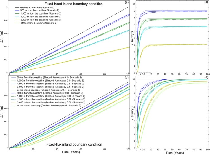
Numerical model results for the change in groundwater level ∆h_t at different distances from the coastline for SLR Scenario 2 and simulations with anisotropy ratios of 0.1 and 0.01 (a) fixed‐head inland boundary condition and (b) fixed‐flux inland boundary condition; and rates of water table rise v for (c) fixed‐head inland boundary condition and (d) fixed‐flux inland boundary condition.

Subsurface Infrastructure Simulations

Simulations including subsurface drainage infrastructure demonstrated that ∆h _t was affected by the drain (Figure 7). In this simulation, rising groundwater levels reached the drain after 49 years (fixed‐head) and 43 years (fixed‐flux) and thereafter, values of ∆h _t were less than values obtained in the simulation without the drain, for all distances from the coastline (Figure  7 b). After 100 years, values of ∆h _t at 500 m from the coastline (i.e., on the coastal side of the drain) were 19% and 45% less than those simulated without a drain (i.e., Scenario 2) for fixed‐head and fixed‐flux, respectively. After 100 years, values of ∆h _t at 1500 m from the coastline (i.e., inland of the drain) were 26% and 53% less than those simulated without a drain for fixed‐head and fixed‐flux, respectively. As such, the drain reduced water table rise more on the inland side than on the coastal side.

Figure 7.

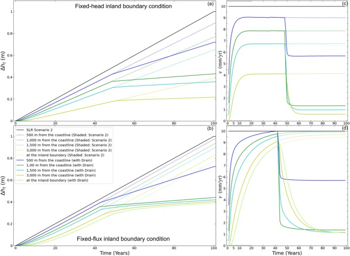
Numerical model results for the change in groundwater level ∆h _t at different distances from the coastline for SLR Scenario 2 and SLR Scenario 2 with subsurface draining infrastructure for (a) fixed‐head inland boundary condition and (b) fixed‐flux inland boundary condition; and rates of water table rise v for (c) fixed‐head inland boundary condition and (d) fixed‐flux inland boundary condition.

Additionally, the drain disrupted the rates of water table rise. As shown in Figure 7c, the equilibrium value of v decreased to a new value once the groundwater levels reached the drain invert for both inland boundary conditions (Figure 7d). After 100 years, values of v at 500 m from the coastline (i.e., on the coastal side of the drain) were 37% and 43% less than that simulated without a drain (i.e., Scenario 2) for fixed‐head and fixed‐flux, respectively. After 100 years, values of v at 1500 m from the coastline (i.e., inland of the drain) were 86% and 88% less than that simulated without a drain for fixed‐head and fixed‐flux, respectively. As such, the drain reduced the rate of water table rise more on the inland side than the coastal side. Additional simulations revealed that when the elevation of the drain increased or the distance of the drain from the coastline increased, the impact on ∆h _t and v was reduced. In simple terms, the location and depth of the drain are essential considerations for managing water table rise in response to SLR, as expected. However, the drainage of the shallow groundwater at the water table in response to SLR may increase inflows in the drain (i.e., groundwater discharge). For fixed‐head inland boundary conditions, as detailed in Morgan (2024), the vulnerability to saltwater intrusion might increase further with the presence of the drain.

Discussion

Impacts to Coastal Shallow Groundwater

Magnitude of Water Table Rise

Results from this study showed that the magnitude of the water table rise (i.e., change in groundwater levels) caused by SLR, at 100 years, is larger for fixed‐flux conditions than for fixed‐head inland boundary conditions for all distances from the coastline, except at the coastline. Additionally, the magnitude of water table rise after 100 years decreased with increasing distance from the coastline. This tends to be more pronounced for fixed‐head inland boundary conditions. These findings are in accordance with those described previously by Morgan (2024) and Masterson and Garabedian (2007), albeit the latter considered an oceanic island setting. In the present study, these relationships were found to apply to all SLR scenarios, that is, instantaneous, linear, or non‐linear SLR.

The magnitude of water table rise after 100 years for a non‐linear SLR scenario (i.e., increasing rates of SLR) was less than that of the scenarios involving linear SLR and instantaneous SLR. That is, simulating a progressive non‐linear SLR scenario will be less conservative in terms of impacts on shallow groundwater levels than either linear gradual or instantaneous SLR. More realistic SLR projections, based on the non‐linear SLR scenario, result in different water table rise estimations.

Rates of Water Table Rise

Results of this study showed that rates of water table rise are always less than rates of SLR, which is in agreement with the findings of Masterson and Garabedian (2007). The present study adds to previous work by showing that varying the magnitude of the (linear) rate of SLR resulted in a proportional change in the rate of water table rise. That is, doubling the rate of SLR resulted in doubling the rate of water table rise, at equilibrium. Also, rates of water table rise in response to SLR after 100 years are larger for fixed‐flux inland boundary conditions. Implications for planners and managers from these findings mean the timing of non‐linear rates of SLR and groundwater rise is important to consider when building and upgrading assets in the coastal zone.

Response Times

In this study, we defined response time as the time required for rates of water table rise to reach equilibrium following the commencement of SLR. It was found that response times for all (gradual linear) rates of SLR are longer for fixed‐flux conditions than for fixed‐head conditions, which agrees with the previous findings of Morgan et al. (2015). Additionally, the present study showed that for fixed‐head conditions, response times are relatively insensitive to the rate of SLR. For fixed‐head conditions and lower rates of SLR, the rate of water table rise at early times was temporarily larger than the final equilibrium value. This can be seen in Figure 4a and 4c. The reason for this is the variable‐density effect of the ocean boundary condition because this is not observed in the freshwater simulations. However, at all times, the magnitude and rates of groundwater rise are always lower than the simulated SLR magnitudes and rates. Importantly, it was found that for fixed‐flux conditions, response times increase with increasing rates of SLR.

From the above, it can be seen that the magnitude and rate of SLR are larger for fixed‐flux conditions than for fixed‐head conditions. Hence, and as pointed out by Befus et al. (2020), the substantial flooding threats from groundwater hazards (i.e., shoaling and emergence) are larger where fixed‐flux conditions occur. However, our study additionally points to a time element whereby for fixed‐flux conditions it takes longer for the system to equilibrate to SLR (i.e., the response time is larger) and hence the maximum impact from SLR may not be experienced for some time (i.e., up to decades). This poses additional challenges to planners and managers of coastal groundwater systems.

Range of Subsurface Infrastructure Problems

Results from this study showed that the presence of subsurface drainage infrastructure interrupted rising groundwater levels after decades for fixed‐head and fixed‐flux conditions at all distances from the coastline. However, between the coastline and the location of the drain, the decrease in magnitude and rate of water table rise is less than beyond the drain. This has implications for infrastructure located near the coast and mitigates rising water tables for areas on the inland side of the drain (Li et al. 2023; Zeydalinejad et al. ²⁰²⁴). Further work is needed to investigate the effect of the drain location on the magnitude and rates of the water table rise.

Globally, engineered water management assets such as drainage and sewage are aging and will interfere with rising shallow groundwater levels. Aging subsurface drainage systems have cracks and have lost their maximum sealed efficiency. If these systems are located historically above the water table, they can become submerged by rising groundwater levels due to SLR in the future (Su et al. 2020; Su et al. ²⁰²²). Infiltration of shallow groundwater into drainage and sewage systems causes additional inflow that is difficult to manage for extreme event conditions. Modeling the impacts of stormwater drains, sewage infiltration, and urban water infrastructure in shallow groundwater environments must be assessed (Zhang and Chui 2019; Sangsefidi et al. ²⁰²³). These models must be integrated with the water table rise response to SLR, especially during extreme rainfall events when the systems may fail, and compound flooding risk will significantly increase. Numerical groundwater modeling studies need to be used more to investigate the transience of subsurface issues in the built environment. Specific findings will improve subsurface infrastructure asset management practices and climate adaptation in coastal areas, also affected by increased exposure to saltwater intrusion, when implementing a dynamic adaptive pathway planning approach (Kool et al. 2020).

A range of subsurface infrastructure problems may emerge due to the transience of water table rise in response to SLR. For subsurface foundations of paved surfaces and buildings, rising and shoaling groundwater can seriously impact their performance and structural competency. Elements of infrastructure composed of reinforced concrete and exposed to saltwater, groundwater level variation, and a wet and dry regime are susceptible to corrosion. Numerical modeling contributes to understanding the effects of SLR and water table rise on subsurface infrastructure and transport networks. Knott et al. (2017) used a groundwater flow model to identify coastal road vulnerability to rising groundwater. Establishing the initial depths to groundwater is crucial to estimating road impacts. Furthermore, the distance from the coastline and surface water serving as groundwater discharge areas will influence infrastructure failure. Generally, hydrogeological information in the coastal areas supports assessment to reduce subsurface infrastructure problems and coastal management for adaptation planning. Further work is needed to investigate tidal effects and extreme events' impacts on these long‐term simulations and the resilience of infrastructure systems.

Another issue is contaminated underground coastal sites that are also at risk of rising groundwater (May et al. 2022; Hill et al. ²⁰²³). Mobile pollutants will likely be exposed in a changing climate and may impact buried infrastructure and urban zones. Further research is needed toward the timing and progression of exposure to groundwater rise at contaminated sites and our study can inform on the preliminary timing and rates of the water table movement in response to SLR.

Limitations

Given that this study is based on the numerical modeling of a simplified and theoretical cross‐section, future research should consider some site‐specific conditions before extrapolating these results to practical management decisions. Groundwater rise can reach the land surface in response to SLR and emerge in real‐world topography. Considerations of different land settings may be valuable to understanding the role of shallow groundwater in compound coastal flooding processes. The comparison between two inland boundary conditions and three SLR forcings covered many possible cases. Sun et al. (2017) used different types of boundary conditions to investigate the effect of SLR on saltwater intrusion. They found that boundaries using general‐head conditions might be more realistic but showed more intermediate impacts. Key results also use more complex projections rather than an incremental approach to SLR. Testing the inland boundary conditions and SLR projections is standard practice in numerical analysis. These are necessary steps to explore and improve the accuracy required to implement efficient adaptation strategies for vulnerable infrastructure.

Initial parameter values used in this assessment were uniform and based on generic coastal groundwater characteristics from the literature (Chang et al. 2011; Lu and Werner ²⁰¹³; Ketabchi et al. ²⁰¹⁶; Mehdizadeh et al. ²⁰¹⁷; Befus et al. ²⁰²⁰). Heterogeneity was not introduced as a variable. Further assessments that account for heterogeneity are recommended. Anisotropy in K will result in a more complex saltwater‐freshwater interface (Pool et al. 2015). However, the results from a change of anisotropy ratio on a linear SLR showed a conservative approach taken by simulating homogeneous and isotropic coastal shallow aquifers and a minimal impact on the magnitude of the water table rise. The rates of water table rise in response to SLR in large anisotropic conditions may be lower than for an ideally modeled isotropic coastal aquifer.

Rising water tables in response to SLR will likely be an escalating issue for the coastal built environment, cities, critical urban infrastructure systems, settlements, and communities along the shoreline (Habel et al. 2020; Magnan et al. ²⁰²²). The modeling approach of this study did not include emergence (i.e., inundation), but the focus was on coastal groundwater rise below the ground surface. Using groundwater numerical modeling supports the information available to plan a practical approach and adaptation for water management in urban and coastal areas (Habel et al. 2017). Chambers et al. (2023) integrated the underground drainage network in a probabilistic modeling approach to estimate the distribution of groundwater flooding projections. Their methodology supported the parametrization of drain elevations, although there is a recognized gap in asset vulnerability studies. Numerical models must be adaptable and represent time‐varying processes to implement decision and management strategies.

Conclusions

Numerical simulations were undertaken to assess the transient water table response to rising mean sea levels using a simple and idealized cross‐sectional model. The modeling approach for shallow unconfined continental coastal settings using SEAWAT quantified and predicted the change in groundwater levels after 100 years for instantaneous and gradual SLR scenarios and the timescale of the water table rise for instantaneous SLR. At all distances from the coastline, the changes in groundwater levels in response to SLR are closely related to SLR, although smaller than the amount of SLR, but not negligible. Models also simulated rates of water table rise for SLR scenarios and different SLR rates, providing a possible range of results for different inland boundary conditions and hydrogeological parameter combinations. The impact of SLR on both the transient response of the change in water table elevation and the rate of water table rise is greatest when the inland boundary is fixed‐flux. The rates of water table rise decreased with distance from the coastline and there were differences in response times from years to decades between the rates of SLR and water table rise depending on rates of SLR. The coastal groundwater response to SLR is faster for high hydraulic diffusivity values for both fixed‐head and fixed‐flux inland boundary conditions. To better characterize the water table changes and the rates of the rise in the coastal zone, it is essential to find out which conditions apply: fixed‐head or fixed‐flux inland boundary conditions. The numerical analysis gave valuable insights into the relationship between SLR and groundwater levels; furthermore, the rates of SLR and water table rise, and the water table response times to SLR.

SLR‐induced groundwater rise induces problems for a range of subsurface infrastructure. A coastal drainage system was simulated using a drain boundary in the numerical groundwater variable‐density flow model. The drain, located at a distance from the coastline, disrupted the rise of the water table and rates of water table rise more on the coastal side than the inland side. Infiltrations of shallow groundwater in coastal subsurface drains can alleviate the impacts of SLR in terms of levels. The changes in water table elevation and rates of water table rise are critical for control and coastal management decisions. However, coastal drainage systems have to be carefully evaluated due to the consequential increase in the vulnerability of saltwater intrusion, which was not evaluated in this study but anticipated in response to SLR.

Authors' Note

The authors do not have any conflicts of interest or financial disclosures to report.

Data Availability Statement

Scripts used throughout this research are available in the dataset by Bosserelle (2024) https://doi.org/10.5281/zenodo.10934463.

References

- Ataie‐Ashtiani, B. , Werner A.D., Simmons C.T., Morgan L.K., and Lu C.. 2013. How important is the impact of land‐surface inundation on seawater intrusion caused by sea‐level rise? Hydrogeology Journal 21, no. 7: 1673–1677. 10.1007/s10040-013-1021-0 [DOI] [Google Scholar]
- Badaruddin, S. , Werner A.D., and Morgan L.K.. 2017. Characteristics of active seawater intrusion. Journal of Hydrology 551: 632–647. 10.1016/j.jhydrol.2017.04.031 [DOI] [Google Scholar]
- Barlow, P.M. 2003. Ground Water in Freshwater‐Saltwater Environments of the Atlantic Coast, 1262. Reston, Virginia: U.S. Geological Survey Circular. https://pubs.usgs.gov/circ/2003/circ1262/ (accessed April 25, 2023). [Google Scholar]
- Befus, K.M. , Barnard P.L., Hoover D.J., Finzi Hart J.A., and Voss C.I.. 2020. Increasing threat of coastal groundwater hazards from sea‐level rise in California. Nature Climate Change 10, no. 10: 946–952. 10.1038/s41558-020-0874-1 [DOI] [Google Scholar]
- Bjerklie, D.M. , Mullaney J.R., Stone J.R., Skinner B.J., and Ramlow M.A.. 2012. Preliminary investigation of the effects of sea‐level rise on groundwater levels in New Haven, Connecticut. U.S. Geological Survey Open‐File Report 2012–1025 46. http://pubs.usgs.gov/of/2012/1025/ (accessed April 25, 2023).
- Bosserelle A.L. 2024. SLR‐induced change in water table elevation. 10.5281/zenodo.10934463. [DOI]
- Bosserelle, A.L. , Morgan L.K., and Hughes M.W.. 2022. Groundwater rise and associated flooding in coastal settlements due to sea‐level rise: A review of processes and methods. Earth's Future 10, no. 7: e2021EF002580. 10.1029/2021EF002580 [DOI] [Google Scholar]
- Burke‐Flask, A. , Stark N., and Rodriguez‐Marek A.. 2021. Addressing Sea Level Rise from the Ground Up: Understanding the Implications for Coastal Geotechnics. Paper presented at Conference on Geo‐Extreme 2021, 393–402. 10.1061/9780784483688.039. [DOI]
- Cazenave, A. , and Cozannet G.L.. 2014. Sea level rise and its coastal impacts. Earth's Future 2, no. 2: 15–34. 10.1002/2013EF000188 [DOI] [Google Scholar]
- Chambers, L.A. , Hemmings B., Cox S.C., Moore C., Knowling M.J., Hayley K., Rekker J., Mourot F.M., Glassey P., and Levy R.. 2023. Quantifying uncertainty in the temporal disposition of groundwater inundation under sea level rise projections. Frontiers in Earth Science 11: 1111065. 10.3389/feart.2023.1111065 [DOI] [Google Scholar]
- Chang, S.W. , Clement T.P., Simpson M.J., and Lee K.‐K.. 2011. Does sea‐level rise have an impact on saltwater intrusion? Advances in Water Resources 34, no. 10: 1283–1291. 10.1016/j.advwatres.2011.06.006 [DOI] [Google Scholar]
- Church, J.A. , and White N.J.. 2011. Sea‐level rise from the late 19th to the early 21st century. Surveys in Geophysics 32, no. 4: 585–602. 10.1007/s10712-011-9119-1 [DOI] [Google Scholar]
- Ghyben, B.W. 1889. Nota in verband met de voorgenomen putboring nabij Amsterdam (notes on the probable results of the proposed well drilling near Amsterdam). The Hague: Tijdschrift van het Koninklijk Instituut voor Ingenieurs 21: 8–22. [Google Scholar]
- Gleeson, T. , Marklund L., Smith L., and Manning A.H.. 2011. Classifying the water table at regional to continental scales: Water table at continental scales. Geophysical Research Letters 38, no. 5. 10.1029/2010GL046427 [DOI] [Google Scholar]
- Grant, A.R.R. , Befus K.M., Hart J.F., Frame M.T., Volentine R., Barnard P., and Knudsen K.L.. 2021. Changes in liquefaction severity in the San Francisco Bay area with sea‐level rise. Geo‐Extreme 2021: 308–317. 10.1061/9780784483695.030 [DOI] [Google Scholar]
- Guo, W. , and Langevin C.D.. 2002. User's guide to SEAWAT; a computer program for simulation of three‐dimensional variable‐density ground‐water flow. U.S. Geological Survey Open‐File Report 2001–434. 10.3133/twri06A7 [DOI]
- Guo, Q. , Zhang Y., Zhou Z., and Zhao Y.. 2020. Saltwater transport under the influence of sea‐level rise in coastal multilayered aquifers. Journal of Coastal Research 36, no. 5: 1040–1049. 10.2112/JCOASTRES-D-19-00189.1 [DOI] [Google Scholar]
- Habel, S. , Fletcher C.H., Rotzoll K., and El‐Kadi A.I.. 2017. Development of a model to simulate groundwater inundation induced by sea‐level rise and high tides in Honolulu, Hawaii. Water Research (Oxford) 114: 122–134. 10.1016/j.watres.2017.02.035 [DOI] [PubMed] [Google Scholar]
- Habel, S. , Fletcher C.H., Rotzoll K., El‐Kadi A.I., and Oki D.S.. 2019. Comparison of a simple hydrostatic and a data‐intensive 3D numerical modeling method of simulating sea‐level rise induced groundwater inundation for Honolulu, Hawai'i, USA. Environmental Research Communications 1, no. 4: 041005. 10.1088/2515-7620/ab21fe [DOI] [Google Scholar]
- Habel, S. , Fletcher C.H., Anderson T.R., and Thompson P.R.. 2020. Sea‐level rise induced multi‐mechanism flooding and contribution to urban infrastructure failure. Scientific Reports 10, no. 1: 1–12. 10.1038/s41598-020-60762-4 [DOI] [PMC free article] [PubMed] [Google Scholar]
- Habel, S. , Fletcher C.H., Barbee M.M., and Fornace K.L.. 2023. Hidden threat: The influence of sea‐level rise on coastal groundwater and the convergence of impacts on municipal infrastructure. Annual Review of Marine Science 16: 81–103. 10.1146/annurev-marine-020923120737 [DOI] [PubMed] [Google Scholar]
- Herbert, E.R. , Boon P., Burgin A.J., Neubauer S.C., Franklin R.B., Ardon M., Hopfensperger K.N., Lamers L.P.M., Gell P., and Langley J.A.. 2015. A global perspective on wetland salinization: Ecological consequences of a growing threat to freshwater wetlands. Ecosphere 6, no. 10: 1–43. 10.1890/ES14-00534.1 [DOI] [Google Scholar]
- Herzberg, A. 1901. Die Wasserversorgung einiger Nordseebider (the water supply on parts of the North Sea coast in Germany). Journal Gabeleucht ung und Wasserversorg ung 44: 815–819, 824–844. [Google Scholar]
- Hill, K. , Hirschfeld D., Lindquist C., Cook F., and Warner S.. 2023. Rising coastal groundwater as a result of sea‐level rise will influence contaminated coastal sites and underground infrastructure. Earth's Future 11, no. 9: e2023EF003825. 10.1029/2023EF003825 [DOI] [Google Scholar]
- Hoover, D.J. , Odigie K.O., Swarzenski P.W., and Barnard P.. 2017. Sea‐level rise and coastal groundwater inundation and shoaling at select sites in California, USA. Journal of Hydrology: Regional Studies 11, no. C: 234–249. 10.1016/j.ejrh.2015.12.055 [DOI] [Google Scholar]
- Hummel, M.A. , Berry M.S., and Stacey M.T.. 2018. Sea level rise impacts on wastewater treatment systems along the U.S. coasts. Earth's Future 6, no. 4: 622–633. 10.1002/2017EF000805 [DOI] [Google Scholar]
- IPCC . 2021. Summary for policymakers. In climate change 2021: The physical science basis. In Contribution of Working Group I to the Sixth Assessment Report of the Intergovernmental Panel on Climate Change (IPCC). Cambridge, United Kingdom: Cambridge University Press. https://www.ipcc.ch/report/ar6/wg1/#TS (accessed April 25, 2023). [Google Scholar]
- IPCC . 2022. Climate change 2022: Impacts, adaptation, and vulnerability. In Summary for Policymakers. Contribution of Working Group II to the Sixth Assessment Report of the Intergovernmental Panel on Climate Change (IPCC), ed. Pörtner H.‐O., Roberts D.C., Tignor M., Poloczanska E.S., Mintenbeck K., Alegría A., Craig M., Langsdorf S., Löschke S., Möller V., Okem A., and Rama B.. Cambridge, United Kingdom: Cambridge University Press. https://www.ipcc.ch/report/ar6/wg2/ (accessed April 25, 2023). [Google Scholar]
- Jiao, J. , and Post V.. 2019. Coastal Hydrogeology. Cambridge, United Kingdom: Cambridge University Press. [Google Scholar]
- Ketabchi, H. , Mahmoodzadeh D., Ataie‐Ashtiani B., and Simmons C.T.. 2016. Sea‐level rise impacts on seawater intrusion in coastal aquifers: Review and integration. Journal of Hydrology 535: 235–255. 10.1016/j.jhydrol.2016.01.083 [DOI] [Google Scholar]
- Knott, J.F. , Elshaer M., Daniel J.S., Jacobs J.M., and Kirshen P.. 2017. Assessing the effects of rising groundwater from sea level rise on the service life of pavements in coastal road infrastructure. Transportation Research Record 2639, no. 1: 1–10. 10.3141/2639-01 [DOI] [Google Scholar]
- Knott, J.F. , Jacobs J.M., Daniel J.S., and Kirshen P.. 2019. Modeling groundwater rise caused by sea‐level rise in coastal New Hampshire. Journal of Coastal Research 35, no. 1: 143–157. 10.2112/JCOASTRES-D-17-00153.1 [DOI] [Google Scholar]
- Kool, R. , Lawrence J., Drews M., and Bell R.. 2020. Preparing for sea‐level rise through adaptive managed retreat of a New Zealand stormwater and wastewater network. Infrastructures 5, no. 11: 92. 10.3390/infrastructures5110092 [DOI] [Google Scholar]
- Langevin, C.D. , D.T. Thorne, Jr , Dausman A.M., Sukop M.C., and Guo W.. 2008. SEAWAT version 4: a computer program for simulation of multi‐species solute and heat transport. U.S. Geological Survey Techniques and Methods, Book 6, Ch. A22. https://pubs.usgs.gov/publication/tm6A22 (accessed April 25, 2023).
- Li, J. , Li X., Liu H., Gao L., Wang W., Wang Z., Zhou T., and Wang Q.. 2023. Climate change impacts on wastewater infrastructure: A systematic review and typological adaptation strategy. Water Research 242: 120282. 10.1016/j.watres.2023.120282 [DOI] [PubMed] [Google Scholar]
- Lu, C. , and Werner A.D.. 2013. Timescales of seawater intrusion and retreat. Advances in Water Resources 59: 39–51. 10.1016/j.advwatres.2013.05.005 [DOI] [Google Scholar]
- Luo, Z. , Kong J., Shen C., Lu C., Xin P., Werner A.D., Li L., and Barry D.A.. 2022. Approximate analytical solutions for assessing the effects of unsaturated flow on seawater extent in thin unconfined coastal aquifers. Advances in Water Resources 160: 104104. 10.1016/j.advwatres.2021.104104 [DOI] [Google Scholar]
- Magnan, A.K. , Oppenheimer M., Garschagen M., Buchanan M.K., Duvat V.K.E., Forbes D.L., Ford J.D., Lambert E., Petzold J., Renaud F.G., Sebesvari Z., van de Wal R.S.W., Hinkel J., and Pörtner H.‐O.. 2022. Sea level rise risks and societal adaptation benefits in low‐lying coastal areas. Scientific Reports 12, no. 1: 10677. 10.1038/s41598-022-14303-w [DOI] [PMC free article] [PubMed] [Google Scholar]
- Masterson J.P. 2004. Simulated interaction between freshwater and saltwater and effects of ground‐water pumping and sea‐level change, Lower Cape Cod aquifer system, Massachusetts. U.S. Geological Survey Numbered Series, Scientific Investigations Report 2004–5014 https://pubs.er.usgs.gov/publication/sir20045014 (accessed April 25, 2023).
- Masterson, J.P. , and Garabedian S.P.. 2007. Effects of sea‐level rise on ground water flow in a coastal aquifer system. Ground Water 45, no. 2: 209–217. 10.1111/j.1745-6584.2006.00279.x [DOI] [PubMed] [Google Scholar]
- May, C. 2020. Rising groundwater and sea‐level rise. Nature Climate Change 10, no. 10: 889–890. 10.1038/s41558-020-0886-x [DOI] [Google Scholar]
- May, C. , Mohan A., Plane E., Ramirez‐Lopez D., Mak M., Luchinsky L., Hale T., and Hill K.. 2022. Shallow Groundwater Response to Sea‐Level Rise: Alameda, Marin, San Francisco, and San Mateo Counties. Pathways Climate Institute and San Francisco Estuary Institute. https://www.sfei.org/documents/shallow‐groundwater‐response‐sea‐level‐rise‐alameda‐marin‐san‐francisco‐and‐san‐mateo (accessed April 25, 2023).
- McCobb, T.D. , and Weiskel P.K., 2003. Long‐term hydrologic monitoring protocol for coastal ecosystems. U.S. Geological Survey Open‐File Report 02–497. https://pubs.usgs.gov/of/2002/ofr02497/
- McGranahan, G. , Balk D., and Anderson B.. 2007. The rising tide: Assessing the risks of climate change and human settlements in low elevation coastal zones. Environment and Urbanization 19, no. 1: 17–37. 10.1177/0956247807076960 [DOI] [Google Scholar]
- Mehdizadeh, S.S. , Karamalipour S.E., and Asoodeh R.. 2017. Sea level rise effect on seawater intrusion into layered coastal aquifers (simulation using dispersive and sharp‐interface approaches). Ocean & Coastal Management 138: 11–18. 10.1016/j.ocecoaman.2017.01.001 [DOI] [Google Scholar]
- Michael, H.A. , Russoniello C.J., and Byron L.A.. 2013. Global assessment of vulnerability to sea‐level rise in topography‐limited and recharge‐limited coastal groundwater systems. Water Resources Research 49, no. 4: 2228–2240. 10.1002/wrcr.20213 [DOI] [Google Scholar]
- Morgan, L.K. 2024. Sea‐level rise impacts on groundwater: Exploring some misconceptions with simple analytic solutions. Hydrogeology Journal 32: 1287–1294. 10.1007/s10040-024-02791-1 [DOI] [Google Scholar]
- Morgan, L.K. , and Werner A.D.. 2014. Seawater intrusion vulnerability indicators for freshwater lenses in strip islands. Journal of Hydrology 508: 322–327. 10.1016/j.jhydrol.2013.11.002 [DOI] [Google Scholar]
- Morgan, L.K. , and Werner A.D.. 2016. Comment on “Closed‐form analytical solutions for assessing the consequences of sea‐level rise on groundwater resources in sloping coastal aquifers”: Paper published in Hydrogeology Journal (2015) 23:1399–1413, by R. Chesnaux. Hydrogeology Journal 24, no. 5: 1325–1328. 10.1007/s10040-016-1398-7 [DOI] [Google Scholar]
- Morgan, L.K. , Werner A.D., and Simmons C.T.. 2012. On the interpretation of coastal aquifer water level trends and water balances: A precautionary note. Journal of Hydrology 470‐471: 280–288. 10.1016/j.jhydrol.2012.09.001 [DOI] [Google Scholar]
- Morgan, L.K. , Stoeckl L., Werner A.D., and Post V.E.A.. 2013a. An assessment of seawater intrusion overshoot using physical and numerical modeling. Water Resources Research 49, no. 10: 6522–6526. 10.1002/wrcr.20526 [DOI] [Google Scholar]
- Morgan, L.K. , Werner A.D., Morris M.J., and Teubner M.D.. 2013b. Application of a rapid‐assessment method for seawater intrusion vulnerability: Willunga Basin, South Australia. In Groundwater in the Coastal Zones of Asia‐Pacific, 205–225. Dordrecht: Springer. 10.1007/978-94-007-5648-9_10 [DOI] [Google Scholar]
- Morgan, L.K. , Bakker M., and Werner A.D.. 2015. Occurrence of seawater intrusion overshoot. Water Resources Research 51, no. 4: 1989–1999. 10.1002/2014WR016329 [DOI] [Google Scholar]
- Oppenheimer, M. , Glavovic B., Hinkel J., van de Wal R., Magnan A.K., Abd‐Elgawad A., Cai R., Cifuentes‐Jara M., Deconto R.M., and Ghosh T.. 2019. Sea level rise and implications for low‐Lying Islands, coasts and communities. In IPCC Special Report on the Ocean and Cryosphere in a Changing Climate, ed. Pörtner H.‐O., Roberts D.C., Masson‐Delmotte V., Zhai P., Tignor M., Poloczanska E., Mintenbeck K., Alegría A., Nicolai M., Okem A., Petzold J., Rama B., and Weyer N.M.. Cambridge, United Kingdom: Cambridge University Press. https://www.ipcc.ch/srocc/ (accessed April 25, 2023). [Google Scholar]
- Passeri, D.L. , Hagen S.C., Medeiros S.C., Bilskie M.V., Alizad K., and Wang D.. 2015. The dynamic effects of sea level rise on low‐gradient coastal landscapes: A review. Earth's Future 3, no. 6: 159–181. 10.1002/2015EF000298 [DOI] [Google Scholar]
- Pool, M. , and Carrera J.. 2011. A correction factor to account for mixing in Ghyben‐Herzberg and critical pumping rate approximations of seawater intrusion in coastal aquifers. Water Resources Research 47, no. 5: 2010WR010256. 10.1029/2010WR010256 [DOI] [Google Scholar]
- Pool, M. , Post V.E., and Simmons C.T.. 2015. Effects of tidal fluctuations and spatial heterogeneity on mixing and spreading in spatially heterogeneous coastal aquifers. Water Resources Research 51, no. 3: 1570–1585. 10.1002/2014WR016068 [DOI] [Google Scholar]
- Post, V.E. , Bosserelle A.L., Galvis S.C., Sinclair P.J., and Werner A.D.. 2018. On the resilience of small‐Island freshwater lenses: Evidence of the long‐term impacts of groundwater abstraction on Bonriki Island, Kiribati. Journal of Hydrology 564: 133–148. 10.1016/j.jhydrol.2018.06.015 [DOI] [Google Scholar]
- Rahimi, R. , Tavakol‐Davani H., Graves C., Gomez A., and Valipour M.F.. 2020. Compound inundation impacts of coastal climate change: Sea‐level rise, groundwater rise, and coastal watershed precipitation. Water 12, no. 10: 2776. 10.3390/w12102776 [DOI] [Google Scholar]
- Ranjbar, A. , Cherubini C., and Saber A.. 2020. Investigation of transient sea level rise impacts on water quality of unconfined shallow coastal aquifers. International Journal of Environmental Science & Technology (IJEST) 17, no. 5: 2607–2622. 10.1007/s13762-020-02684-2 [DOI] [Google Scholar]
- Rasmussen, P. , Sonnenborg T., Goncear G., and Hinsby K.. 2013. Assessing impacts of climate change, sea level rise, and drainage canals on saltwater intrusion to coastal aquifer. Hydrology and Earth System Sciences 17, no. 1: 421–443. 10.5194/hess-17-421-2013 [DOI] [Google Scholar]
- Rotzoll, K. , and Fletcher C.H.. 2013. Assessment of groundwater inundation as a consequence of sea‐level rise. Nature Climate Change 3, no. 5: 477–481. 10.1038/nclimate1725 [DOI] [Google Scholar]
- Sangsefidi, Y. , Bagheri K., Davani H., and Merrifield M.. 2023. Data analysis and integrated modeling of compound flooding impacts on coastal drainage infrastructure under a changing climate. Journal of Hydrology 616: 128823. 10.1016/j.jhydrol.2022.128823 [DOI] [Google Scholar]
- Shi, W. , Lu C., Ye Y., Wu J., Li L., and Luo J.. 2018. Assessment of the impact of sea‐level rise on steady‐state seawater intrusion in a layered coastal aquifer. Journal of Hydrology 563: 851–862. 10.1016/j.jhydrol.2018.06.046 [DOI] [Google Scholar]
- Shi, W. , Lu C., and Werner A.D.. 2020. Assessment of the impact of sea‐level rise on seawater intrusion in sloping confined coastal aquifers. Journal of Hydrology 586: 124872. 10.1016/j.jhydrol.2020.124872 [DOI] [Google Scholar]
- Smith, S.M. , and Medeiros K.C.. 2019. Recent groundwater and lake‐stage trends in Cape Cod National Seashore: Relationships with sea level rise, precipitation, and air temperature. Journal of Water and Climate Change 10, no. 4: 953–967. 10.2166/wcc.2018.016 [DOI] [Google Scholar]
- Strack, O.D.L. 1976. A single‐potential solution for regional interface problems in coastal aquifers. Water Resources Research 12, no. 6: 1165–1174. 10.1029/WR012i006p01165 [DOI] [Google Scholar]
- Strack, O.D.L. 1989. Groundwater mechanics. Englewood Cliffs, New Jersey: Prentice Hall. [Google Scholar]
- Su, X. , Liu T., Beheshti M., and Prigiobbe V.. 2020. Relationship between infiltration, sewer rehabilitation, and groundwater flooding in coastal urban areas. Environmental Science and Pollution Research 27, no. 13: 14288–14298. 10.1007/s11356-019-06513-z [DOI] [PubMed] [Google Scholar]
- Su, X. , Belvedere P., Tosco T., and Prigiobbe V.. 2022. Studying the effect of sea level rise on nuisance flooding due to groundwater in a coastal urban area with aging infrastructure. Urban Climate 43: 101164. 10.1016/j.uclim.2022.101164 [DOI] [Google Scholar]
- Sukop, M.C. , Rogers M., Guannel G., Infanti J.M., and Hagemann K.. 2018. High temporal resolution modeling of the impact of rain, tides, and sea level rise on water table flooding in the Arch Creek basin, Miami‐Dade County Florida USA. Science of the Total Environment 616‐617: 1668–1688. 10.1016/j.scitotenv.2017.10.170 [DOI] [PubMed] [Google Scholar]
- Sun, D.‐m. , Niu S.‐x., and Zang Y.‐g.. 2017. Impacts of inland boundary conditions on modeling seawater intrusion in coastal aquifers due to sea‐level rise. Natural Hazards 88, no. 1: 145–163. 10.1007/s11069-017-2860-0 [DOI] [Google Scholar]
- Voss, C.I. , and Souza W.R.. 1987. Variable density flow and solute transport simulation of regional aquifers containing a narrow freshwater‐saltwater transition zone. Water Resources Research 23, no. 10: 1851–1866. 10.1029/WR023i010p01851 [DOI] [Google Scholar]
- Walter, D.A. , McCobb T.D., Masterson J.P., and Fienen M.N.. 2016. Potential effects of sea‐level rise on the depth to saturated sediments of the Sagamore and Monomoy flow lenses on Cape Cod, Massachusetts. U.S. Geological Survey Scientific Investigations Report 2016–5058 Version 1.1. https://pubs.usgs.gov/sir/2016/5058/sir20165058.pdf (accessed April 25, 2023).
- Watson, T.A. , Werner A.D., and Simmons C.T.. 2010. Transience of seawater intrusion in response to sea level rise. Water Resources Research 46, no. 12: 2010WR009564. 10.1029/2010WR009564 [DOI] [Google Scholar]
- Webb, M.D. , and Howard K.W.F.. 2011. Modeling the transient response of saline intrusion to rising sea‐levels. Ground Water 49, no. 4: 560–569. 10.1111/j.1745-6584.2010.00758.x [DOI] [PubMed] [Google Scholar]
- Werner, A.D. , and Simmons C.T.. 2009. Impact of sea‐level rise on sea water intrusion in coastal aquifers. Ground Water 47, no. 2: 197–204. 10.1111/j.1745-6584.2008.00535.x [DOI] [PubMed] [Google Scholar]
- Werner, A.D. , Ward J.D., Morgan L.K., Simmons C.T., Robinson N.I., and Teubner M.D.. 2012. Vulnerability indicators of sea water intrusion. Ground Water 50, no. 1: 48–58. 10.1111/j.1745-6584.2011.00817.x [DOI] [PubMed] [Google Scholar]
- Yu, X. , Yang J., Graf T., Koneshloo M., O'Neal M.A., and Michael H.A.. 2016. Impact of topography on groundwater salinization due to ocean surge inundation. Water Resources Research 52, no. 8: 5794–5812. 10.1002/2016WR018814 [DOI] [Google Scholar]
- Yu, X. , Luo L., Hu P., Tu X., Chen X., and Wei J.. 2022. Impacts of sea‐level rise on groundwater inundation and river floods under changing climate. Journal of Hydrology 614: 128554. 10.1016/j.jhydrol.2022.128554 [DOI] [Google Scholar]
- Zamrsky, D. , Karssenberg M.E., Cohen K.M., Bierkens M.F.P., and Oude Essink G.H.P.. 2020. Geological heterogeneity of coastal unconsolidated groundwater systems worldwide and its influence on offshore fresh groundwater occurrence. Frontiers in Earth Science 7, no. 339: 339. 10.3389/feart.2019.00339 [DOI] [Google Scholar]
- Zamrsky, D. , Oude Essink G.H.P., and Bierkens M.F.P.. 2024. Global impact of sea level rise on coastal fresh groundwater resources. Earth's Future 12, no. 1: 2023EF003581. 10.1029/2023EF003581 [DOI] [Google Scholar]
- Zeydalinejad, N. , Javadi A.A., and Webber J.L.. 2024. Global perspectives on groundwater infiltration to sewer networks: A threat to urban sustainability. Water Research 262: 122098. 10.1016/j.watres.2024.122098 [DOI] [PubMed] [Google Scholar]
- Zhang, K. , and Chui T.F.M.. 2019. A review on implementing infiltration‐based green infrastructure in shallow groundwater environments: Challenges, approaches, and progress. Journal of Hydrology 579: 124089. 10.1016/j.jhydrol.2019.124089 [DOI] [Google Scholar]
Associated Data
This section collects any data citations, data availability statements, or supplementary materials included in this article.