Determination of causal connectivities of species in reaction networks

Abstract

We present an approach to the determination of causal connectivities and part of the kinetics of complex reaction systems. Our approach is based on analytical and computational methods for studying the effects of a pulse change of concentration of a chemical species in a reaction network, either at equilibrium or in a nonequilibrium stationary state. Such disturbances generally propagate through a few species, depending on the values of the kinetic coefficients, before being broadened and dissipated. This short range gives a local probe of the kinetics and connectivity of the reaction network. The range of propagation also indicates species to perturb in further experiments. From piecing together these local connectivities, the global structure of the network can be constructed. The experimental design allows deduction of both reaction orders and rate constants in many cases. An example of the usefulness of the approach is illustrated on a model of a part of glycolysis.

Standard methods used for the study of the structure of reaction networks include determination of the stoichiometry and kinetics of individual steps followed by hypothesizing reaction mechanisms and testing them against such measurements; perturbations of reaction systems with first-order kinetics to determine the constant rate matrix (1); and introduction of radioactive tracers to determine reaction connectivities (2). In addition, several approaches are used to infer causal relationships in genetic networks; however, most of these techniques are applicable only to Boolean networks (3–8). Our work has taken several different approaches to this problem in nonequilibrium systems (9–15), all based on not dissecting the system but maintaining all interactions. Using fluctuating input concentrations, we have shown how correlations among species measured in the entire system may be used to construct distances among species and from this infer information on the reaction pathway (11, 12). This correlation metric construction gives a hierarchy of influence in a system and identifies weakly coupled subsystems; causal connectivities can be obtained with more difficulty. The methods outlined in the present paper give causal reaction connectivities of measured species and regulatory features of a reaction network through analyses of responses of a system to pulse perturbations. For these techniques, the concentrations of species affected by a given pulse need to be measured in time. The measurement resolution required, both in concentration and time, depends on the stationary state concentration values, the rates of reaction, and the connectivity of the reaction network. However, adequate estimates of concentration detection levels may be based on stationary state values, and estimates of time resolution levels may be based on the time of appearance of extrema after a pulse perturbation. Typically, a modest number of time measurements, often 10 or fewer, is sufficient to approximate extrema locations and values. From these measurements, both reaction orders and rate constants of an empirical rate equation may be deduced in many cases. The global structure of the reaction network is obtained by piecing together these local connectivities. We start with straightforward examples to show the simplicity of the approach and then indicate the applicability to complicated cases. An example of the usefulness of the approach is illustrated on a model of a part of glycolysis.

The number of species that need to be pulsed to deduce the causal connectivities of the species, and hence the reaction pathway, depends on the complexity of the reaction system; we do not address the issue of rules applicable to this point. At most, all the species of the system need to be pulsed, which will lead to all connectivities, but frequently fewer than all are necessary. We illustrate in the Appendix how connectivity may be obtained by using few perturbations in a simple example.

Method and Theory

The application of the impulse perturbation method to a reaction network consists of changing the concentration of a given species over a short time and then observing the concentration responses X induced in it and other species. A plot of the deviation in concentration from the stationary state value, X − X_s, against time shows that for unbranched chains of reactions, the (first) extrema in the concentration of species are ordered along the time axis with decreasing amplitude according to the number of reaction steps separating that species from the initially perturbed species. Pulses propagate strongly, i.e., with large amplitude, in the direction of net reaction velocity and weakly in the reverse direction. As an example, we consider the case of an unbranched chain of reversible first-order reactions:

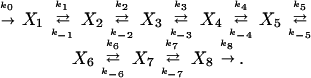1

For first-order reactions, it is convenient to study the relative change in concentration u = (X − X^s) = X^s as a function of time, u(t). These reduced variables exhibit relatively simple relations at extrema. Equating the time derivative of u_i(t) to zero at the time of an occurrence of an extrema t_i, we obtain a relation between the extremum value u_i(t_i) and the values of the relative concentrations of other species u_j≠i(t_i). In the following, we often abbreviate the extremum value as u and omit explicit reference to time t_i. From the deterministic kinetic equations for Eq. 1, we obtain

2

where the coefficient α is less than one,

3

j_f = k_i−1X is the steady state forward flow into X_i; and j_T = j_f + j_r is the total flow into X_i. This relation shows that a maximum in u_i occurs between the curves for the preceding and succeeding species; i.e., in addition to time ordering of extrema, the values at maxima of (relative deviations of) species are also ordered according to the number of reaction steps separating that species from the initially perturbed species. The usefulness of these relations follows from their geometric interpretation and independence from rate values. Measurements to investigate connectivity of species through reactions need only determine times of occurrences of extrema and concentration values of species at them. Fig. 1a shows the propagation of a pulse following a pulse perturbation of the first species X₁ in the chain of reactions. Using relative deviations of concentrations, we verify that maxima, as well as values at maxima, are ordered according to the number of reaction steps separating that species from the initially perturbed species. The effect of perturbing a species in the middle of the chain is shown in Fig. 1b. In this case, the pulse propagates with large amplitude in the direction of the overall reaction velocity and weakly in the opposite direction. For segments of systems in which there is not a large net reaction velocity, e.g., for subsystems close to equilibrium, a pulse perturbation induces extrema in neighboring species that are similar in magnitude: a pulse propagates equally in both directions away from the perturbation source.

Figure 1.

Plots of the relative deviation in concentration from the stationary state versus time for all the species of the mechanism in Eq. 1. The maxima are ordered according to the number of reaction steps separating that species from the initially perturbed species. In b, the pulse propagates with large amplitude in the direction of the overall reaction velocity and weakly in the opposite direction.

More complicated mechanisms are studied through an analysis of times and values of extrema in concentration changes of species. These values give information about local connectivities and kinetics (e.g., feedback, higher-order kinetics). Several observations, which often hold, may be used as guidelines in the initial construction of connectivities of species in a reaction network. (i) The time of an extremum increases as the number of reaction steps separating that species from the initially perturbed species increases, unless some species act as effectors in distant reactions. (ii) Conversely, the initial curves of concentration changes of a species with time approach the time axis as the number of reaction steps separating that species from the initially perturbed species increases (in the absence of effectors). (iii) Species that are directly connected through reactions to the initially perturbed species exhibit nonzero initial slopes. (iv) Species that are not directly connected through reactions to the initially perturbed species exhibit zero initial slopes. (v) All responses are positive deviations from the stationary state unless there is a feedback, feedforward, or higher-order (>1) kinetic step. (vi) For short times, prior to the exit of material from the pulse to the surroundings of the reaction system, the concentration change of the pulse is conserved: the sum of deviations of concentrations (weighted by stoichiometric coefficients) must be constant and equal to the change in concentration of the initial pulse. This property is useful in confirming that all species produced from the pulse through reactions have been detected and can help in determining correct stoichiometric coefficients. (vii) When it is possible to identify the rate expressions for reaction steps, then kinetic constants may be estimated from the values of the concentrations of species at an extremum. In the above example, the value of α, Eq. 3, may be estimated from extrema, which gives the ratio k_i−1/k_−i.

We have investigated the effects of some geometrical arrangements and rate expressions on the conditions for extrema. The geometries considered include (i) straight chains, (ii) branched chains, i.e., several chains converging and diverging from a given species, (iii) positive and negative feedback and feedforward, and (iv) a cycle of reactions. The rate expressions treated include: (i) first- and second-order kinetics, (ii) generalized mass-action kinetics (for small perturbations), and (iii) uni-uni enzyme catalyzed reactions (Michaelis–Menten). The analytic solutions for these simplify considerably for the case of irreversible reactions.

First-Order Kinetics.

We consider a set of reactions that may be described by first-order or pseudo-first-order kinetics; e.g., reversible Michaelis–Menten kinetics in which the substrate concentration is low. Specifically, the reactions either produce or consume a species X:

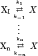4

Then the rate expression for X is

5

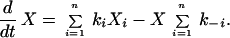
The evolution of the relative deviation from the stationary state, u = (X − X^s) = X^s, may be written

6

where α_i = j_i/j_T, j_i = k_iX, and j_T = ∑j_i. We note that the sum of coefficients is equal to one: ∑α_i = 1. An extremum in u occurs when the above derivative with respect to time is zero, which for this system results in the expression:

7

This abbreviated form for the relation between values of variables at an extremum of u omits explicit inclusion of the time variable; implicit in this expression is the evaluation of all variables at time t* at which du/dt = 0.

From this expression, we have the result that an extremum u* occurs within (the convex hull of) the curves u_i for the species that produce X. For example, in the case of a chain of irreversible reactions X₁ → X → X₂, the extremum u* occurs on u₁; the curve for the species that produces X. Another example is the case of irreversible reactions in which two species, X₁ and X₂, separately produce X; and X produces one product X₃. Then u* occurs between the curves for the species that produce X, u₁, and u₂, and at such a point the coefficients sum to one: α₁ + α₂ = 1.

Fig. 2 shows a diagram of converging chains of irreversible first-order reactions. Perturbation of species X₁ causes a pulse to propagate through the sequence X₂; X₃; X₄; X₅, Fig. 3a; perturbation of species X₈ causes the pulse to propagate through the sequence X₇; X₆; X₃; X₄; X₅, Fig. 3b. In each of these figures, we note that aside from the branch species X₃, the maximum value (of the relative deviation) of a species occurs on the curve for the species that produces it. For the branch species, the maximum value of u₃ is equal to α_i u_i, where i is 2 or 6, depending on whether the pulse propagate through species X₂ or X₆, i.e., whether X₁ or X₈ is perturbed. The sum of the coefficients α₂ + α₆ is equal to one and is a useful check on the correct number of converging chains at X₃. These relations may be extended to networks of nearly irreversible reactions, where they hold to within a correction that is the order of the reverse rate divided by the forward rate.

Figure 2.

Chemical reaction mechanism for converging chains of irreversible first-order reactions. The rates of production of species X₁ and X₈ are held constant at 0.1 and 0.5, respectively. [X_i]₀ denotes the stationary state concentration of species X_i.

Figure 3.

Plots of relative deviation in concentration versus time for species of the mechanism in Fig. 2. In a, a perturbation of the concentration of species X₁ causes a pulse to propagate through the sequence X₂; X₃; X₄; X₅; in b, perturbation of species X₈ causes the pulse to propagate through the sequence X₇; X₆; X₃; X₄; X₅. With the exception of the branch species X₃, the maximum value (of the relative deviation) of a species occurs on the curve for the species that produces it. For the branch species, the maximum value of u₃ is equal to α_i u_i, where i is 2 or 6, depending on whether the pulse originates from species X₂ or X₆. The coefficients α₂ and α₆ are the relative contributions of the branch fluxes to the total flux: α₂ = j₁/(j₁ + j₂) and α₆ = 1 − α₂.

Cyclic reaction systems may be investigated by using the above methods. Such systems are composed of chains of reactions that form a closed loop; inputs and outputs are branch points of the loop. Using Eq. 7, the linear and branch points of the system may be identified through appropriate perturbations. Another class of systems for which the above methods and results are directly applicable is those in which radioactive tracer species are introduced. If a tracer is added so that the total concentration of the species is constant, then the response of the tracer obeys first-order kinetics.

Generalized Mass-Action Kinetics.

The propagation of pulses, and in particular the conditions for extrema, may also be described for higher-order reaction kinetics.

For the case of two different species reacting, we take the following reaction scheme:

8

The condition for an extremum in one of the species u_b involved in the bimolecular reaction may easily be derived. For small reverse velocities, j₋₁/j_T ≪ 1; the condition reduces to

9

where

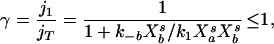10

and j₋₁ = k₋₁X, j_T = j_−b + j₁ = k_−bX + k₁XX. If the second-order reaction rate is much greater than the rate of the other reaction that destroys X_b, then we have j_−b/j₁ ≪ 1, and Eq. 9 reduces to u^*_b = −u_a/(1 + u_a). The approximate condition for an extremum in the product u₂, for small reverse rate coefficient j_−b/j₁ ≪ 1

11

To illustrate an application of these conditions, we consider an impulse change of concentration of species X_a in Eq. 8. Following this perturbation, the concentration of species X_b decreases below the stationary state value and reaches a minimum value given by Eq. 9. The concentration of the product of the reaction increases and reaches a maximum value given by Eq. 11. For small perturbations, the maximum value u^*₂ is the sum of u_a and u_b.

Generalized mass-action kinetics may be treated similarly. We consider the case in which the creation and consumption of a species X₁ are each single reactions with power rate laws (we assume the reverse rates of these reactions are small):

12

The sets of species that produce X₁; (X_a, X_b, … , X_l); and the set of products, (X₁, X₂, … , X_n); are not necessarily disjoint. These types of rate equations, called S-systems, have been applied to the analysis of biochemical pathways and genetic networks (16). Then for small deviations from the stationary state, the equation may be linearized, which leads to the following condition at an extremum in u₁ (du₁/dt = 0)

13

That is, as in the case of irreversible first- and second-order kinetics, at an extremum the values of the reduced variables are linearly related with coefficients determined only by the exponents η. For these and similar systems, the exponents η may be determined through experiments that probe the effects of perturbing different species that are involved in reactions that create X₁.

We illustrate the application of this relation by using a sequence of first- and second-order reactions given in Fig. 4. In this example, where a single species is produced and destroyed at each reaction step, the above relation simplifies to u^*₁ ≈ (η_a/η₁)u_a. An impulse perturbation of X₁ results in the responses shown in Fig. 5. Connectivities between species are reflected in the times of extrema of the relative deviations: u₂ follows u₁, … , u₈ follows u₇. The relations between the variables at extrema give ratios of exponents. For example, X₂ is produced through a first-order reaction involving X₁ and consumed through a second-order reaction of X₂. This results in the relation u^*₂ ≈ (η₁/η₂)u₁ = (1/2)u₁ at an extremum in X₂; i.e., the order of the second reaction is determined from the extremum relation. The other relations are similarly determined at extrema of Fig. 4 and are u^*₃ ≈ 2u₂, u^*₆ ≈ (1/2)u₅, and u^*₇ ≈ 2u₆. Using these relations along with other information, such as initial rate studies, the rate coefficients k_i may be determined.

Figure 4.

Chemical reaction mechanism of a linear chain of coupled first- and second-order reactions. The order of a reaction is given by the stoichiometry.

Figure 5.

Plots of relative deviation in concentration versus time for species of the mechanism in Fig. 4. A pulse perturbation of the concentration of species X₁ results in the responses shown. The pulse propagates through the chain with maxima of relative deviations of species ordered according to the positions of species in the chain. From the plot we find the relations: u^*₂ ≈ (1/2)u₁, u^*₃ ≈ 2u₂, u^*₆ ≈ (1/2)u₅, and u^*₇ ≈ 2u₆; and u^*₇ ≈ 2u₆; the values of these coefficients may be related to the orders of the reactions through Eq. 14.

Feedback and Feedforward.

Feedback and feedforward effects arise in chemical reaction networks from a variety of mechanisms. The rate of a reaction may be either increased or decreased by an effector species not directly involved in the reaction; the location of this effector species in the network may either precede (feedforward) or succeed (feedback) the reaction. A general mechanism may be treated by linearizing the equations about a stationary state. For these cases, absolute deviations from the stationary state are more useful than relative deviations, because the species directly affected by the reaction show symmetric deviations. We consider an effector species X_eff either promoting or inhibiting the reaction X_i → X_i+1, and all reverse processes are assumed negligible. We assume a general rate function f(X_i; X_eff) for the feedforward or feedback that has nonzero derivatives with respect to X_i and X_eff at the stationary state. Then the linearized rate equations are

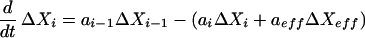14

15

where ΔX_i denotes the deviation in concentration of species X_i from the stationary state value and a_i = ∂f/∂X_i, a_eff = ∂f/∂X_eff. If a_eff > 0 (a_eff < 0), then X_eff acts as an activator (inhibitor) of the reaction. The effector species X_eff and its influence on the reaction may be identified through a (direct or indirect) perturbation of the concentration of X_eff. After such a perturbation, for short times such that changes in X_i; X_i−1, and X_i+1 are small in comparison to ΔX_eff, deviations in species X_i and X_i+1 are mirror images about the time axis:

16

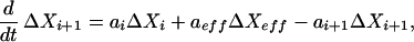
[Assuming ΔX_eff and the coefficients a are O (1) and that ΔX_i(Δt)/ΔX_f is small O (ɛ), then Δt = O (ɛ) for this relation to hold.] The extrema are ordered with the extremum of ΔX_i+1 occurring before that of ΔX_i, independent of the sign of a_eff (assuming that X_effdoes not influence X_i−1 significantly, e.g., X_eff does not directly produce X_i−1). This may be shown as follows: if a_eff > 0, then a_i ΔX_i + a_effΔX_eff starts out positive, which implies a consumption of X_i by Eq. 15, and decreases to zero at the minimum of ΔX_i; Eq. 15 (the influence of X_i−1 is negligible if it is not influenced directly by X_eff). According to Eq. 16, ΔX_i+1 initially increases, because a_i ΔX_i + a_eff ΔX_eff > 0, and reaches a maximum value at the crossing of the curves a_i+1 ΔX_i+1 and a_i ΔX_i + a_eff ΔX_eff which occurs before the minimum of ΔX_i (at a_i ΔX_i + a_eff ΔX_eff = 0). Similarly, if a_eff < 0; then a_i ΔX_i + a_eff ΔX_eff starts out negative and increases to zero at the maximum of ΔX_i; following the previous argument, the minimum of ΔX_i+1 occurs before the maximum of ΔX_i. This ordering of extrema allows the identification of the direction of the net reaction velocity X_i → X_i+1.

An example of a system with positive feedback is shown in Fig. 6. The associated rate equations are integrated for a perturbation in concentration of X₁ and X₇; the absolute deviation of concentration from the stationary state is given in Fig. 7 a and b, respectively. Fig. 7a shows maxima of species occurring in the order of species in the chain of reactions X₁ → X₈. Species X₃ falls below the stationary state value, which indicates a possible feedback effect from one of the later species. A trial perturbation of X₇, Fig. 7b, shows that X₃ and X₄ are mirror images about the time axis for short times, and their initial slopes are nonzero. These observations indicate that X₇ activates the reaction from X₃ to X₄ (the peak of X₄ occurs before that of X₃, implying that X₃ precedes X₄ in the reaction sequence).

Figure 6.

Chemical reaction mechanism illustrating positive feedback in a linear chain of irreversible first-order reactions. The rate of production of species X₁ is held constant at v_f.

Figure 7.

Plots of deviation in concentration ΔX from the stationary state value versus time for the species of the mechanism in Fig. 6. In a, a perturbation of the concentration of species X₁ causes a pulse to propagate through the linear chain X₂, X₃, ⋯, X₈; the deviation of species X₃ falls below the stationary state value, which indicates a possible feedback effect from one of the species farther in the chain. In b, a perturbation of species X₇ causes the initial slopes of the deviations in X₃, X₄, and X₈ to be nonzero and the deviations in X₃ and X₄ to be mirror images about the time axis (for short times); these observations indicate that X₇ activates the reaction from X₃ to X₄ (because the peak of X₄ occurs before that of X₃, implying that X₃ precedes X₄ in the reaction sequence) and is the precursor to X₈. The maximum deviations are approximately 10% of the stationary state values or larger, except X₄ in b, which is 2% (the stationary state values of X₁ − X₈ are 0.05, 0.0125, 0.0166, 0.1, 0.0166, 0.025, 0.01, and 0.1, respectively).

Enzyme-Catalyzed Reactions.

Many segments of biochemical pathways may be modeled as unbranched chains consisting of enzyme-catalyzed reactions. We concentrate on a chain in which the kinetics are described by the irreversible Michaelis–Menten equation:

17

The rate of the relative deviation of S₂ is given by

18

For small deviations from the stationary state, we linearize the equations, use the stationary state condition for the relation between S and S, and obtain the following expression for an extremum in u₂:

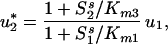19

where K_m1 = (k₋₁ + k₂)/k₁; K_m3 = (k₋₂ + k₃)/k₂: We see that, unlike the case of first-order reactions, the value of u^*₂ may be greater or less than u₁. If the concentrations of the substrates are much smaller than the corresponding Michaelis constants, i.e., S/K_m1 ≪ 1; S/K_m3 ≪ 1, then kinetics reduce to first-order, and the above relation becomes that for the case of irreversible first-order kinetics, u^*₂ = u₁.

An Example: The Glycolytic Pathway

We present an application of some of the methods outlined above to a model of the glycolytic pathway. The model we use includes many of the known activations and inhibitions of enzymes by metabolites, Fig. 8. The HKase reaction is assumed to operate at constant rate, which neglects the influence of ATP and glucose 6-phosphate. The concentrations of glucose, lactic acid, and the total adenine nucleotide pool are kept constant; the AKase reaction is assumed to be at equilibrium. Prior to the application of a pulse, the system is in a nonequilibrium stationary state. We refer to ref. 17 for details concerning the assumptions and the derivation of rate equations. There are five independent variables: fructose 6-phosphate (F6P), fructose 1,6-bisphosphate (FDP), phosphoenolpyruvate (PEP), pyruvate (PYR), and ATP; in the following, we label the variables 1–5, respectively. Our parameter values are the same as those in ref. 17, except for the input rate, which we take as V = 1.5 mM/min.

Figure 8.

Chemical reaction mechanism for an abbreviated model of the glycolytic pathway. The mechanism includes many of the known activations and inhibitions of enzymes by metabolites. Broken lines indicate activation ⊕ or inhibition ⊝ of enzymes by metabolites. The abbreviations for the enzymes are hexokinase (HK), phosphofructokinase (PFKase), and pyruvate kinase (PKase); the abbreviations for the five independent variables are fructose 6-phosphate (F6P), fructose 1,6-bisphosphate (FDP), phosphoenolpyruvate (PEP), pyruvate (PYR), and ATP (in the following figure, these are labeled 1–5, respectively).

Fig. 9 a–d shows time series for the absolute deviations of species with impulse perturbations of F6P (1), FDP (2), PEP (3) and ATP (5); solutions were obtained from numerical integration of the model equations. In Fig. 9a, the response to an impulse perturbation of (1) is shown. The variables exhibit extrema in the following order in time 2, 3, 4; the variable 5 exhibits both a minimum and a maximum. Variables 3 and 4 have zero initial slopes, which is consistent with their production from 2: the deviation in 2 starts at zero, which implies that the velocity of 2 into any of its products, e.g., (3, 4), is initially zero. Also, for short times, the deviations in 3 and 4 are mirror images about the time axis, which indicates that the conversion between 3 and 4 is affected by 2 (if 1 were to affect this conversion, then the initial slope of 3 and 4 would be nonzero). A separate perturbation of 4, which is not shown, does not produce a significant response in 3; therefore, it is inferred that 3 produces 4. A verification that 1 is converted to 4 is shown in Fig. 10a, where the sum of the deviations in concentrations ΔX₁ + ΔX₂ + (ΔX₃ + ΔX₄)/2 is slowly decaying in time. This indicates an approximate conservation of mass among these species. We note from this conservation that each molecule of species 2 produces two molecules of species 3, which in turn produces (one molecule of) species 4. The initial slope of 5 in Fig. 9a is equal to minus that of 2, which shows that 5 is consumed in equal numbers to 2 produced. In summary, from the responses to a perturbation of 1 (and 4), we have the results: 1 produces 2, 2 produces 3, 2 activates the conversion of 3 to 4, 3 produces 4, and 5 is consumed in the conversion of 1 to 2 (with the stoichiometric ratio of species 5 to species 2 being 1:1).

Figure 9.

Plots of time series for the absolute deviations in concentrations of species of the mechanism in Fig. 8 with impulse perturbations of F6P (1), FDP (2), PEP (3) and ATP (5). From an analysis of the responses to these perturbations, we deduce: 1 produces 2, 2 produces 3, 2 activates the conversion of 3 to 4, 3 produces 4, and 5 is consumed in the conversion of 1 to 2 (with the stoichiometric ratio of species 5 to species 2 being 1:1); the conversion of 1 to 2 is highly irreversible; 5 is produced at the same rate as 4 in the reaction 3 to 4; 5 is consumed at the same rate as 2 is produced, which indicates that 5 is a cosubstrate for the reverse reaction of 3 to 2; 5 inhibits the reaction of 1 to 2 and the reaction of 3 to 4. In each of the response plots, the perturbation is 10% of the stationary state value; responses are approximately several percent of the stationary state values or larger, except X₅, which is in a and b (the stationary state values of X₁ − X₅ are 0.091, 0.200, 2.70, 3.00, and 30.0, respectively).

Figure 10.

Plots of time series for sums of deviations in concentrations for the species of the mechanism in Fig. 8. In a, the concentration of species X₁ is perturbed; in b, the concentration of species X₃ is perturbed. Plot a shows that the sum of the deviations ΔX₁ + ΔX₂ + (ΔX₃ + ΔX₄)/2 is slowly decaying in time. From this conservation, we infer that species 2 produces two molecules of species 3, which produces species 4. Plot b shows a similar transient conservation of mass in species 2, 3, and 4 following a perturbation of 3; the initial flow is from 3 to (1/2) 2 and over a longer time from 3 to 4.

Fig. 9b shows responses to an impulse perturbation of species 2. The initial slopes of 3 and 4 are nonzero, which indicates that 2 has a direct effect on (activates) the conversion of 3 to 4; the initial effect of 2 is to activate the reaction from 3 to 4 (and slowly produce 3). The minimum in 3 precedes the maximum in 4 following a perturbation of 2, which indicates that 2 directly produces 3 and shifts the minimum of 3 (which would occur after the maximum in 4 without this direct production) to an earlier time. Species 1 does not respond to the perturbation, which shows that the conversion of 1 to 2 is highly irreversible. The initial slope of species 5 is equal to that of 4, which shows that 5 is produced at the same rate as 4 in the reaction 3 to 4. The new information from this perturbation is the production of 5 in this latter reaction.

Fig. 9c shows responses to an impulse perturbation of species 3. Both 2 and 4 have nonzero initial slopes, which shows that 3 produces both 2 and 4. The small amplitude of 2 indicates that the reaction 2 to 3 is reversible. New information is also contained in the initial time series for 2 and 5: 5 is consumed at the same rate as 2 is produced, which indicates that 5 is a cosubstrate for the reverse reaction of 3 to 2. Fig. 10b shows a transient conservation of mass in species 2, 3, and 4; the initial flow is from 3 to (1/2) 2 and over a longer time from 3 to 4.

Fig. 9d shows responses to an impulse perturbation of species 5. The minus signs in the figure denote reflection of the deviations about the time axis. The increase of 1 and decrease of 2 indicate that 5 inhibits the reaction 1 to 2, without affecting the rate of 2 to 3. The opposite rates of 3 and 4 indicate that 5 also inhibits the conversion of 3 to 4.

From the above analysis of the propagation of pulses in the glycolytic pathway, we may construct the reaction scheme shown in Fig. 11. This diagram captures the topology of the reaction network and many of the effectors. Further studies of the adenine nucleotides would help determine the role of the other effector (AMP) and other substrates, such as ADP, for each reaction.

Figure 11.

A simplified mechanism constructed from the analysis of Figs. 9 and 10. This diagram captures the topology of the reaction network in Fig. 8 and many of the effectors.

Discussion

From an analysis of responses of reaction systems to pulse perturbations in concentrations of chemical species (applied to stationary state), we are able to construct the dominant kinetic structure of reaction networks. The level of information obtained depends on the number of species that are accessible to measurement and external perturbation. While correct deductions about the order of a particular reaction necessitates all involved species be identified and measured, much of the network structure can be obtained with less information. For example, in some biochemical systems, the kinetics of reactions may be treated as first-order or pseudo first-order; in these cases, identification of ordering of species in linear chains of reactions and branch points follows from analysis of extrema following appropriate perturbations. In these systems, it is also possible to determine the location of species that have not been measured in the network and the number of chains converging or diverging from a branch point from locations of extrema and sums of relative fluxes, respectively. Blind tests of the methods presented here are needed. These studies will be performed on realistic models of biological pathways and should help determine the numbers of measurements needed to construct networks of a given level of complexity.

Appendix

Much can be learned, by simple deduction, from measuring the responses to a pulse perturbation of a given species in a reaction mechanism. Consider the following case: a flow from the main branch into a side branch given in Fig. 12. Perturbations of only three chemical species, X₁, X₂, X₆, and calculations of the responses of the other species suffice to deduce the causal connectivities of the species and the reaction mechanism.

Figure 12.

Chemical reaction mechanism for diverging chains of first-order reactions. The rates of production of species X₁ are held constant at 0.1.

References

- 1.Wei J, Prater J D. Advances in Catalysis. Vol. 13. New York: Academic; 1962. pp. 204–390. [Google Scholar]
- 2.Boudart M. Kinetics of Chemical Processes. Englewood Cliffs, NJ: Prentice-Hall; 1968. [Google Scholar]
- 3.Liang S, Fuhrman S, Simogyi R. Pacific Symposium on Biocomputing. 1998;3:18–29. [PubMed] [Google Scholar]
- 4.Weaver D C, Workman C T, Stormo G D. Pacific Symposium on Biocomputing. 1999;4:112–123. doi: 10.1142/9789814447300_0011. [DOI] [PubMed] [Google Scholar]
- 5.Akutsu T, Miyano S, Kuhara S. Pacific Symposium on Biocomputing. 1999;4:17–28. doi: 10.1142/9789814447300_0003. [DOI] [PubMed] [Google Scholar]
- 6.Akutsu T, Miyano S, Kuhara S. Pacific Symposium on Biocomputing. 2000;5:293–304. doi: 10.1142/9789814447331_0028. [DOI] [PubMed] [Google Scholar]
- 7.Ideker T E, Thorsson V, Karp R M. Pacific Symposium on Biocomputing. 2000;5:305–316. doi: 10.1142/9789814447331_0029. [DOI] [PubMed] [Google Scholar]
- 8.D'Haeseleer P, Liang S, Simogyi R. Bioinformatics. 2000;16:707–726. doi: 10.1093/bioinformatics/16.8.707. [DOI] [PubMed] [Google Scholar]
- 9.Eiswirth M, Freund A, Ross J. J Phys Chem. 1991;95:1294–1299. [Google Scholar]
- 10.Gilman A, Ross J. Biophys J. 1995;69:1321–1333. doi: 10.1016/S0006-3495(95)79999-4. [DOI] [PMC free article] [PubMed] [Google Scholar]
- 11.Arkin A, Ross J. J Phys Chem. 1995;99:970–979. [Google Scholar]
- 12.Arkin A, Shen P, Ross J. Science. 1997;277:1275–1279. [Google Scholar]
- 13.Ross J, Vlad M. Annu Rev Phys Chem. 1999;50:51–78. doi: 10.1146/annurev.physchem.50.1.51. [DOI] [PubMed] [Google Scholar]
- 14.Vlad M O, Moran M, Ross J. Physica A. 2000;278:504–525. [Google Scholar]
- 15.Tsuchiya T, Ross J. J Phys Chem A. 2001;105:4052–4058. [Google Scholar]
- 16.Irvine D H, Savageau M A. SIAM J Num Anal. 1990;27:704–735. [Google Scholar]
- 17.Termonia Y, Ross J. Proc Natl Acad Sci USA. 1981;78:2952–2956. doi: 10.1073/pnas.78.5.2952. [DOI] [PMC free article] [PubMed] [Google Scholar]