Effective Non-IID Degree Estimation for Robust Federated Learning in Healthcare Datasets

Abstract

Building unbiased and robust machine learning models using datasets from multiple healthcare systems is critical for addressing the needs of diverse patient populations. However, variations in patient demographics and healthcare protocols across systems often lead to significant differences in data distributions. Not Independent and Not Identically Distributed (non-IID) data presents a major challenge in developing effective federated learning (FL) frameworks. This study proposes a method to estimate the non-IID degree between datasets and introduces three metrics (variability, separability, and computational time) to evaluate and compare the performance of non-IID degree estimation methods. We developed a novel non-IID FL algorithm that incorporates the proposed non-IID degree estimation index as regularization into existing FL algorithms for acute kidney injury risk (AKI) prediction. Our results demonstrate that the proposed method for estimating non-IID degree outperforms previous approaches by effectively identifying differences in data distributions between datasets, consistently producing similar estimates of non-IID degree when evaluating different subsamples from the same dataset, requiring significantly less computational time, and providing better interpretability. Finally, we showed that the proposed non-IID FL algorithm achieves higher test accuracy than local learning, concurrent FL algorithms, and centralized learning for the AKI prediction task.

Introduction

Non-independent and non-identically distributed (non-IID) data poses challenges in deploying machine learning (ML) models across healthcare settings, where data heterogeneity is inherent due to variations in patient demographics, clinical practices, geographical locations, environmental and socioeconomic factors [1, 2].

A ML model which fits data from one healthcare system may not generalize to data from other healthcare systems due to these distribution differences. Consider an asthma risk prediction model (Fig. 1): data from metropolitan hospitals reflects populations with high exposure to vehicle emissions and dust mites, along with ready access to healthcare services, while rural populations face different risk factors such as biomass fuel exposure and limited healthcare access, despite potential protective factors from farm environments. A model trained on urban hospital data may therefore perform poorly when applied to rural populations due to these significant environmental, socioeconomic, and geographical differences. Such data distribution shifts exemplify the non-IID challenge in healthcare ML, highlighting the difficulty of developing unbiased, generalizable models for diverse populations. When two electronic health record (EHR) datasets have large non-IID degree, failure to quantify this distribution shift could make ML model produces biased predictions and unintended discrimination [3, 4].

Fig. 1.

An example of Non-IID data challenge in healthcare ML: consider building a ML model to predict asthma risk

This issue is particularly critical as the importance of ensuring fairness in healthcare ML grows, especially in addressing social determinants of health (SDoH) in ML applications [5, 6]. Able to robustly estimate non-IID degree can help institutes to identify and mitigate potential model deployment risks when apply to historically underserved populations [7] that ML models may unintentionally discriminate or perform poorly.

Although federated learning (FL) [8] offers ML algorithms designed to address non-IID challenges, robust methods for estimating non-IID degree between local datasets are not widely used. Currently, FL and ML healthcare research lacks standard methods for estimating non-IID degree in EHR data, and a widely adopted evaluation framework to systematically assess different non-IID degree estimation methods.

Previous ML model-based approaches used to measure distribution difference in ML, which rely on deep learning model outputs or weights to estimate non-IID degree, require model training, lack interpretability, and are highly sensitive to model architecture and hyperparameter choices. These limitations make current methods unreliable for healthcare applications where robust non-IID degree estimation is crucial for ensuring model fairness and generalizability.

This study addresses the challenges of current non-IID degree estimation methods by:

1. Proposing a statistical-based non-IID degree estimation approach, using statistical hypothesis testing and effect size measurements to quantify the distribution shift between local EHR tabular datasets. Our novel approach addresses limitations of previous methods by providing an interpretable, model-agnostic method that handles mixed data types and enables statistical significance testing of distribution differences. This method targets the fully overlapping attribute skew and label distribution skew where the same features are present in all local datasets. We demonstrated the validity of our non-IID estimation method through experiments which showed the positive correlation relationship between the estimated non-IID degree and ML model testing error.

2. Proposing three metrics to systematically evaluate and compare the performance of non-IID degree estimation methods: non-IID degree variability, data distribution separability, and computational time. To the best of the authors’ knowledge, this represents the first systematic approach for evaluating non-IID estimation methods in FL. Using these metrics, compared to previous non-IID degree estimation methods, our non-IID estimation method achieved lowest non-IID degree variation under different sampling percentages, highest data distribution separability, and lowest computational time.

3. Developing a FL algorithm which incorporates non-IID degree into FL training process. Specifically, we utilize non-IID degree as a regularization term to mitigate the adverse effects of data heterogeneity on local model updates. By assigning higher regularization values to local nodes with higher non-IID degrees, our approach limits the impact of divergent local updates, promoting more robust global model. Results showed our non-IID FL algorithm outperformed centralized learning, local learning, and concurrent FL methods including federated averaging (FedAvg) [9], FedProx [10], and Mime Lite [11], when evaluated on three datasets: Medical Information Mart for Intensive Care (MIMIC)-III [12], MIMIC-IV [13], and eICU Collaborative Research Database (eICU-CRD) [14], in acute kidney injury (AKI) risk prediction.

The remainder of this paper is organized as follows. Section II introduces non-IID issues in ML. Section III details the proposed non-IID estimation method, the metrics to evaluate non-IID estimation method, and the non-IID FL algorithm. Section IV describes the experimental design, datasets used, and data preprocessing process. Section V presents experimental results and performance evaluation of non-IID estimation methods. Finally, Section VI summarizes this study and the future work.

Background and Related Work

This section examines non-IID data in machine learning through three aspects. We begin by defining non-IID characteristics from both data distribution and model objective perspectives. We then review methods for estimating non-IID degree of model-based approaches while examining their limitations. Finally, we survey federated learning techniques developed to address non-IID challenges in distributed learning environments.

Two aspects of IID in Machine Learning

ML methods generally assume that training data and testing data are IID [15, 16]. IID data is usually defined from two aspects. From data aspect, IID data is identically distributed such that each sample $S_i=\left(x_i,,,y_i\right)$ is taken from the same probability distribution $p\left(S_i\right)\sim P\left(x,,,y\right)$ where $x$ represents features and $y$ represents label. Further, IID data is also independently distributed such that any two samples are independent events, where $p\left(S_i,,,S_j\right)=p\left(S_i\right)·p\left(S_j\right)$. Empirically, for a dataset, non-IID could come from quantity skew, label skew (e.g., label distribution skew, label preference skew, temporal skew), and attribute skew (e.g., non-overlapping attribute skew, partial overlapping attribute skew, full overlapping attribute skew) [17].

From ML model aspect, assume there are $K$ clients with the set of indexes of samples $S_k$ on client $k$ and sample size $n_k=\left|S_k\right|$. The objective of a FL system can be defined as:

$$f\left(\omega \right)=\sum _{k=1}^K\frac{n_k}{n}{F}_k\left(\omega \right),where{F}_k\left(\omega \right)=\frac{1}{n_k}\sum _{i\in S_k}{f}_i\left(\omega \right)$$ 1

where $f_i\left(\omega \right)$ is the prediction on sample $S_i=\left(x_i,,,y_i\right)$ with model parameter $\omega$. If the partition $S_k$ was created by distributing the training sample over the clients uniformly and randomly, IID data satisfies the expectation $E_{S_k}{[F}_k\left(\omega \right)]=f\left(\omega \right)$ of the global model $F_k\left(\omega \right)$ with an approximation to finite summations of the local model $f_i\left(\omega \right)$ [9].

Non-IID estimation: Direct Distribution Difference Measures Approach

This subsection provides an overview of selected methods commonly used in ML for distribution difference measurements, categorizing them into distance measures, similarity measures, and entropy-based measures [18, 19].

Similarity measures assess the closeness between distributions. Cosine Similarity evaluates the directional alignment between vectors while disregarding their magnitude differences. The Jaccard Index measures similarity between finite sample sets, while the Weighted Jaccard Similarity extends this to numerical values: $J_w=\frac{{\sum }_{i=1}^n\text{min}(u_i,v_i)}{{\sum }_{i=1}^n\text{max}(u_i,v_i)}$. While this extension accounts for value magnitudes, its sensitivity to outliers can lead to biased estimates of distribution differences.

Distance measures calculate the separation between distributions. The Minkowski family of distances defines the distance between two vectors $u$ and $v$ in $n$-dimensional space as: $d\left(u,,,v\right)={({\sum }_{i=1}^n{|u_i-v_i|}^q)}^{\frac{1}{q}}$, where $q=1$ gives Manhattan Distance and $q=2$ yields Euclidean Distance. These metrics treat each dimension independently, neglecting feature interactions. The Mahalanobis Distance addresses this limitation by incorporating a covariance matrix: $d_M\left(u,,,v\right)=\sqrt{{\left(u,-,v\right)}^T{V}^{-1}\left(u,-,v\right)}$ where $V=\left[\begin{array}{cc}cov(u,u)& cov(u,v)\\ cov(v,u)& cov(v,v)\end{array}\right]$. However, this measure assumes linear relationships between variables, which limits its effectiveness for datasets with nonlinear feature interactions.

Entropy-based measures quantify the difference between probability distributions. Kullback–Leibler (KL) Divergence measures how one probability distribution $w$ diverges from a reference distribution $z$: $d_{\mathit{KL}}(w\Vert z)={\sum }_{i=1}^n{w}_i\text{log}\frac{w_i}{z_i}$. While powerful, KL Divergence is asymmetric and unbounded. Jensen-Shannon (JS) Divergence [20] addresses KL Divergence’s asymmetry and unboundedness: $d_{\mathit{JS}}(w\left(\Vert ,z\right)=\frac{1}{2}{d}_{\mathit{KL}}(w\left(\Vert ,M\right)+{\frac{1}{2}d}_{\mathit{KL}}(z\Vert M)$, where $M=\frac{w+z}{2}$ is the midpoint distribution. However, JS Divergence relies on the assumption that $M$ reasonably represents both distributions, which may not hold when distributions are substantially different.

These measures face several limitations when applied to estimating non-IID degrees in tabular datasets: (1) Many measures struggle with mixed data types common in EHRs that contain both continuous and categorical variables. (2) Most measures evaluate features independently, missing important interdependencies that could indicate non-IID characteristics. (3) It is challenging to determine whether calculated distribution differences are statistically significant, making it difficult to establish meaningful thresholds for non-IID detection.

Non-IID Estimation: Machine Learning Model Based Approach

Current non-IID degree estimation methods in ML are model-based, focusing on measuring non-IID degree between images using deep learning (DL) model outputs or weights.

He et al. [21] proposed using model outputs to measure non-IID degree between images. They use the activations from a convolutional neural network’s (CNN) last hidden layer to measure non-IID degree between training $D_{\mathit{TR}}=\left(X_{\mathit{TR}},,,Y_{\mathit{TR}}\right)$ and testing $D_{\mathit{TE}}=\left(X_{\mathit{TE}},,,Y_{\mathit{TE}}\right)$ data in an image class, where $X$ represents the images and $Y$ represents the labels. Given a feature extractor $g\left(·\right)$ and a class $C$, the non-IID index $NI\left(C\right)$ between $D_{\mathit{TR}}^C=\left(X_{\mathit{TR}}^C,,,Y_{\mathit{TR}}^C\right)$ and $D_{\mathit{TE}}^C=\left(X_{\mathit{TE}}^C,,,Y_{\mathit{TE}}^C\right)$ is defined in Eq. (2), where $X^c=X_{\mathit{TR}}^C\bigcup X_{\mathit{TE}}^C$, $\sigma$ represents standard deviation used to normalize the scale of features, $\stackrel{-}{(·)}$ is the first order moment, and $\Vert ·\Vert$ represents the 2-norm. Their results show that higher $NI\left(C\right)$ value led to higher testing errors across image classes.

$$NI\left(C\right)={\Vert \frac{\stackrel{-}{g(X_{\mathit{TR}}^C)}-\stackrel{-}{g(X_{\mathit{TE}}^C)}}{\sigma \left(g,(,X^C,)\right)}\Vert }_2$$ 2

Li et al. [22] adapted $NI\left(C\right)$ [21] into the Client-Wise Non-IID Index (CNI), as shown in Eq. (3), where $D={\bigcup }_{i=1}^N{D}_i$, $D_i^k$ represents the data belonging to the kth class in $D_i$, and $\left|C_i\right|$ is the number of image classes in $D_i$. The main difference between $NI\left(C\right)$ and $CNI\left(C_i\right)$ is that $NI\left(C\right)$ must train different feature extractors $g\left(·\right)$ to compute non-IID degrees for different datasets; while $CNI\left(C\right)$ replaces the feature extractors $g\left(·\right)$ in $NI\left(C\right)$ with a fixed encoder $En\left(·\right)$.

$$CNI\left(C_i\right)={\Vert \frac{{\mathrm{\Sigma }}_k\frac{1}{\left|C_i\right|}\stackrel{-}{En\left(D_i^k\right)}-\overline{{\mathrm{\Sigma }}_l\frac{1}{{\left|C_j\right|}_{j\ne i}}\stackrel{-}{En\left(D_j^l\right)}}}{\sigma \left(E,n,\left(D\right)\right)}\Vert }_2$$ 3

Zhao et al. [23] proposed using DL model weights to measure non-IID degree between images. They trained FL models on 2-class (each client has 2 image classes) and 1-class (each client has 1 image class) data. They found that higher non-IID degrees led to lower test accuracy and observed greater weight divergence in non-IID data compared to IID data when using stochastic gradient descent.

These model-based non-IID estimation approaches rely on trained DL models, which have several disadvantages: (1) They require DL model training prior to non-IID degree estimation. (2) The dependence on DL makes these approaches not model-agnostic. (3) The estimated non-IID degree is heavily influenced by model hyperparameters and architecture choices. (4) The estimated non-IID degree lacks interpretability because the black-box nature of DL models.

Federated Learning Methods Tackling Non-IID Challenges

Medical data is often restricted and difficult to centralize for model training due to privacy concerns and regulatory constraints. FL [9] enables participating institutions to train models locally on their own data. The local models are then transmitted to a central server for aggregation. The server combines the parameters of these models to create an updated global model, which is subsequently shared with the participants for further local training. This iterative process enhances overall model performance while preserving data privacy.

Training FL models on non-IID data face three main challenges: communication overhead, aggregation optimization, and model performance [24]. The communication challenge stems from the need for frequent model updates due to heterogeneous client data, resulting in increased network delays and bandwidth consumption. Researchers have proposed various solutions, including model compression techniques like SlimFL [25] and client clustering methods such as CAFL [26] to optimize bandwidth utilization.

The aggregation optimization challenge arises from local model parameter heterogeneity and issues with global model convergence and training biases. Solutions include intelligent client selection mechanisms (e.g., CSFedAvg [27]), adaptive aggregation methods (e.g., DOCS [28] and FedGroup [29]), and clustering-based approaches such as Kalman filter-based clustering FL [30] to enhance training stability.

Model performance challenge comes from data heterogeneity across clients. Approaches to address this challenge can be broadly classified into three categories [31, 32]: data-based, algorithm-based, and framework-based. (1) Data-based approaches focus on resolving data disparities through data augmentation and sharing (e.g., training a global generative adversarial network to generate synthetic data that supplements local datasets [33, 34], or leveraging global variational autoencoders to share latent space distributions with local nodes for data generation [35]), and data selection (e.g., clustering clients with similar data distributions into subgroups to train multiple specialized global models [36]). (2) Algorithm-based approaches focus on improving model training through enhanced update and aggregation strategies, as well as model hyperparameter designs, such as regularization techniques (e.g., using contrastive loss between local and global model as regularization term [37, 38]), novel model architectures (e.g., FL gradient boosting decision tree [39], FL-enabled fine-tuning of local large language models for better prompt engineering [40]), and optimizers (e.g., replacing standard stochastic gradient descent optimizer with adaptive optimizers, improve training dynamics [41, 42]). (3) Framework-based approaches integrate FL with other learning paradigms, such as federated transfer learning [43] for image feature extraction to improve downstream task performance, federated reinforcement learning [44] for optimizing resource allocation control in edge computing, and federated meta-learning [45] for enhanced few-shot image prediction.

Algorithms

The algorithms section describes the proposed non-IID estimation method, non-IID evaluation metrics, and non-IID FL algorithm.

Non-IID Estimation Algorithm

This section introduces the proposed non-IID estimation method to evaluate feature distribution difference of two input datasets. Algorithm 1 shows the pseudo-code of the proposed non-IID degree estimation method.

Algorithm 1.

Non-IID Degree Quantification Process

Since the features can be either numerical or categorical, the proposed non-IID degree estimation method uses different calculations for each variable type. Numerical variables are values which contain continuous values, such as blood pressure value and heart rate, while categorical variables contain a finite number of distinct groups, such as gender and blood type.

Assume two given datasets $D_1={\left\{\left({\mathcal{X}}_{1,i},=,\{x_{1,i}^1,x_{1,i}^2,x_{1,i}^3,\cdots ,x_{1,i}^N\},,,y_{1,i},\in ,{\mathcal{Y}}_1\right)\right\}}_{i=1}^1$ and $D_2={\left\{\left({\mathcal{X}}_{2,i},=,\{x_{2,i}^1,x_{2,i}^2,x_{2,i}^3,\cdots ,x_{2,i}^N\},,,y_{2,i},\in ,{\mathcal{Y}}_2\right)\right\}}_{i=1}^2$ with $n_1$ and $n_2$ sample size, where $x_1$ and $x_2$ represent the samples in $D_1$ and $D_2$, and ${\mathcal{Y}}_1$ and ${\mathcal{Y}}_2$ are the labels. All samples in $D_1$ and $D_2$ have the same feature space $\mathcal{F}=\{f_1,f_2,\cdots ,f_N\}$. We first group all features into two nonoverlapping groups based on their variable types. The first group ${\mathcal{F}}^{\mathit{nv}}=\{f_1^{\mathit{nv}},f_2^{\mathit{nv}},\cdots ,f_{n_{\mathit{nv}}}^{\mathit{nv}}\}$ includes the features with the numerical variables and the second group ${\mathcal{F}}^{\mathit{cv}}=\{f_1^{\mathit{cv}},f_2^{\mathit{cv}},\cdots ,f_{n_{\mathit{cv}}}^{\mathit{cv}}\}$ includes the features with the categorical variable, where feature number of each group is $n_{\mathit{nv}}=|{\mathcal{F}}^{\mathit{nv}}|$ and $n_{\mathit{cv}}=|{\mathcal{F}}^{\mathit{cv}}|$, also $n_{\mathit{nv}}+n_{\mathit{cv}}=N$.

For each feature $f_i^{\mathit{nv}}$ in the numerical variable group, Welch’s $t$-test in Eq. (4) is used to obtain the corresponding feature distribution difference, where ${\overline{x}}_{D_1}^{f_i^{\mathit{nv}}}=\left({\sum }_{k=1}^1,v_{1,k}^{f_i^{\mathit{nv}}}\right)/n_1$ and ${\overline{x}}_{D_2}^{f_i^{\mathit{nv}}}=\left({\sum }_{k=1}^2,v_{2,k}^{f_i^{\mathit{nv}}}\right)/n_2$ are the average values of the numerical variables $f_i^{\mathit{nv}}$ for all samples in each dataset. $S_{D_1}^2=\left({\sum }_{k=1}^1,\left({v_{1,k}^{f_i^{\mathit{nv}}}-\overline{x}}_{D_1}^{f_i^{\mathit{nv}}}\right)\right)/n_1$ and $S_{D_2}^2=\left({\sum }_{k=1}^2,\left({v_{2,k}^{f_i^{\mathit{nv}}}-\overline{x}}_{D_2}^{f_i^{\mathit{nv}}}\right)\right)/n_2$ are the sample standard deviations. We then count the number of numerical variables $n_{\mathit{sig}}^{\mathit{nv}}$ which $t_{f_i^{\mathit{nv}}}$ values reach the predefined significance level by the $p$ value with Bonferroni correction. Finally, for numerical features with corrected $p$ values reach the predefined significance level, we measure effect size using the Cohen’s $d$ (value range [0, 1]) in Eq. (5). The pseudo-code for calculating the statistical results for the features in the numerical variable group starts from line 05 to 08 in Algorithm 1.

$$t_{f_i^{\mathit{nv}}}=\left({\overline{x}}_{D_1}^{f_i^{\mathit{nv}}},-,{\overline{x}}_{D_2}^{f_i^{\mathit{nv}}}\right)/\sqrt{\left(\frac{S_{D_1}^2}{n_1},+,\frac{S_{D_2}^2}{n_2}\right)},wherei=\text{1,2},\cdots ,n_{\mathit{nv}}$$ 4

$$d_{f_i^{\mathit{nv}}}=\frac{\left|{\overline{x}}_{D_1}^{f_i^{\mathit{nv}}},-,{\overline{x}}_{D_2}^{f_i^{\mathit{nv}}}\right|}{S},whereS=\sqrt{\frac{\left(n_1,-,1\right)S_{D_1}^2+\left(n_2,-,1\right)S_{D_2}^2}{n_1+n_2-2}}$$ 5

For each feature $f_i^{\mathit{cv}}$ in the categorical variable group, Pearson’s ${\chi }^2$ test in Eq. (6) is used to obtain the corresponding feature distribution difference, where $\Vert f_i^{\mathit{cv}}\Vert$ is the number of possible values for the processing feature $f_i^{\mathit{cv}}$. $O_{r,c}$ is the observation of one element of a two-dimensional array according to the number of datasets and the number of possible values for the processing feature $f_i^{\mathit{cv}}$. Therefore, the dimension of the two-dimensional matrix consists of 2 rows and $\Vert f_i^{\mathit{cv}}\Vert$ columns. $E_{r,c}$ is the theoretical frequency calculated by Eq. (7). We then count the number of categorical variables $n_{\mathit{sig}}^{\mathit{cv}}$ which ${\chi }_{f_i^{\mathit{cv}}}^2$ values reach the predefined significance level by the $p$ value with Bonferroni correction. Finally, for categorical features with corrected $p$ values reach the predefined significance level, we measure effect size using the Cramér’s $V$ (value range [0, 1]) measurement in Eq. (8). Lines 10 to 13 in Algorithm 1 contain the pseudo-code for calculating the statistical results for the features in the categorical variable group.

$${\chi }_{f_i^{\mathit{cv}}}^2=\sum _{r=1}^2\sum _{c=1}^{\Vert f_i^{\mathit{cv}}\Vert }\frac{{\left(O_{r,c},-,E_{r,c}\right)}^2}{E_{r,c}},wherei=\text{1,2},\cdots ,n_{\mathit{nv}}$$ 6

$$E_{r,c}=\frac{\left({\sum }_{c=1}^{\Vert f_i^{\mathit{cv}}\Vert },O_{r,c}\right)\times \left({\sum }_{r=1}^2,O_{r,c}\right)}{2\times \Vert f_i^{\mathit{cv}}\Vert }$$ 7

$$V_{f_i^{\mathit{cv}}}=\sqrt{{\chi }_{f_i^{\mathit{cv}}}^2/\left(2\times \Vert ,f_i^{\mathit{cv}},\Vert \right)}$$ 8

After all the features are processed, if the value of $n_{\mathit{sig}}^{\mathit{nv}}$ and $n_{\mathit{sig}}^{\mathit{cv}}$ are both zero, the final non-IID degree $\mathcal{D}$ between two datasets $D_1$ and $D_2$ is equal to zero. Otherwise, the non-IID degree $\mathcal{D}$ is calculated by Eq. (9) which value ranges [0, 1] ($0\le n_{\mathit{sig}}^{\mathit{nv}}+n_{\mathit{sig}}^{\mathit{cv}}\le N$, and $0\le {\sum }_{i=1}^{\mathit{nv}}\left(d_{f_i^{\mathit{nv}}},/,d_{f_i^{\mathit{nv}}}^M\right)+{\sum }_{i=1}^{\mathit{cv}}\left(V_{f_i^{\mathit{cv}}},/,V_{f_i^{\mathit{cv}}}^M\right)\le N$), where $d_{f_i^{\mathit{nv}}}^M$ and $V_{f_i^{\mathit{cv}}}^M$ are the maximum effect size of all the features in the numerical and categorical groups separately (see Eq. (10)). Lines 14 to 18 in Algorithm 1 describes the process of final non-IID degree determination.

$$\mathcal{D}=\frac{\left(n_{\mathit{sig}}^{\mathit{nv}},+,n_{\mathit{sig}}^{\mathit{cv}}\right)+{\sum }_{i=1}^{\mathit{nv}}\left(d_{f_i^{\mathit{nv}}},/,d_{f_i^{\mathit{nv}}}^M\right)+{\sum }_{i=1}^{\mathit{cv}}\left(V_{f_i^{\mathit{cv}}},/,V_{f_i^{\mathit{cv}}}^M\right)}{2N}$$ 9

$$d_{f_i^{\mathit{nv}}}^M=\underset{i\in \left\{\text{1,2},,,\cdots ,,,n_{\mathit{sig}}^{\mathit{nv}}\right\}}{\text{max}}{d}_{f_i^{\mathit{nv}}},V_{f_i^{\mathit{cv}}}^M=\underset{i\in \left\{\text{1,2},,,\cdots ,,,n_{\mathit{sig}}^{\mathit{cv}}\right\}}{\text{max}}{V}_{f_i^{\mathit{cv}}}$$ 10

Performance Evaluation Metrics for the Non-IID Estimation Method

This section introduces three evaluation metrics for assessing the efficacy of non-IID estimation method: Variability, Separability, and Computational Time.

The first metric, Variability $\mathit{VA}$, evaluates the ability of a non-IID estimation method to maintain its robustness under different random sampling percentages. For a robust method, different random samples of the same underlying dataset should not produce dramatically different measures of non-IID degree. A lower non-IID variability indicates that the method can provide more consistent, reliable, and reproducible results when applied repeatedly for a benchmark dataset.

Given one benchmark dataset $D_b$ and a test set $D_t$, we random sampling the benchmark dataset and the test set $k$ times under a random sampling percentage $s^i$, where $i$ indicates different random sampling percentages and $i=1,2,\cdots ,h$, to create $k$ random sampled benchmark datasets $D_b^{s_j^i}$ and $k$ random sampled test sets $D_t^{s_j^i}$, where $j=1,2,\cdots ,k$. The non-IID degrees between $D_b^{s_j^i}$ and $D_t^{s_j^i}$ is ${\mathcal{D}}_{b,t}^{s_j^i}$. The ${\mathit{VA}}_b^i$ in Eq. (11) is the standard deviation $\sigma$ of the non-IID degrees ${\mathcal{D}}_{b,t}^{s_j^i}$. The Variability $\mathit{VA}$ is the average of $V{A}^i$ under different random sampling percentage.

$$VA=\frac{1}{h}\left(\sum _{i=1}^h,{\mathit{VA}}_b^i\right),whereV{A}^i=\sigma \left({\mathcal{D}}_{b,t}^{s_j^i}\right)$$ 11

The second metric, Separability ${\mathit{SE}}_b$, is used to evaluate how the ability of a non-IID estimation method to separate different data distributions. A higher separability value indicates the method has higher capacity to separate different data distributions.

Assume there are $N$ test sets $D_{t_n}^{s_j^i}$ where $n=1,2,\cdots ,N$. The non-IID degree between benchmark dataset $D_b^{s_j^i}$ and $D_{t_n}^{s_j^i}$ is ${\mathcal{D}}_{b,t_n}^{s_j^i}$. The Separability ${\mathit{SE}}_b$ is calculated by 1 minus the normalized sum of overlapping range values for any two selected normalized non-IID arrays from $N$ test sets; the number of overlapping range values is $C_2^N$. For example, we only use two test sets, denoted as $D_{t_1}^{s_j^i}$ and $D_{t_2}^{s_j^i}$. The non-IID degrees for these two test sets with the $D_b^{s_j^i}$ are ${\mathcal{D}}_{b,t_1}^{s_j^i}=\{{\mathcal{D}}_{b,t_1}^{s_1^i},{\mathcal{D}}_{b,t_1}^{s_2^i},...,{\mathcal{D}}_{b,t_1}^{s_k^i}\}$ and ${\mathcal{D}}_{b,t_2}^{s_j^i}=\{{\mathcal{D}}_{b,t_2}^{s_1^i},{\mathcal{D}}_{b,t_2}^{s_2^i},...,{\mathcal{D}}_{b,t_2}^{s_k^i}\}$, and ${\mathcal{D}}_{b,t_{\text{1,2}}}^{s_j^i}=\{{\mathcal{D}}_{b,t_1}^{s_j^i},{\mathcal{D}}_{b,t_2}^{s_j^i}\}$. The calculation of ${\mathit{SE}}_b$ begins by normalizing the values in ${\mathcal{D}}_{b,t_1}^{s_j^i}$ and ${\mathcal{D}}_{b,t_2}^{s_j^i}$ into range between [0, 1] using the largest non-IID value ${\mathcal{D}}_{b,t_{\text{1,2}}^M}^i=\mathit{max}\left({\mathcal{D}}_{b,t_{\text{1,2}}}^{s_j^i}\right)$ to produce normalized ${\mathcal{D}}_{b,t_1}^{\prime s_j^i}=\frac{{\mathcal{D}}_{b,t_1}^{s_j^i}}{{\mathcal{D}}_{b,t_{1,2}^M}^i}$ and ${\mathcal{D}_{}^{\prime }}_{b,t_2}^{s_j^i}=\frac{{\mathcal{D}}_{b,t_2}^{s_j^i}}{{\mathcal{D}}_{b,t_{\text{1,2}}^M}^i}$. Four values, $M_1=max({\mathcal{D}_{}^{\prime }}_{b,t_1}^{s_j^i})$, $m_1=min({\mathcal{D}_{}^{\prime }}_{b,t_1}^{s_j^i})$, $M_2=max({\mathcal{D}_{}^{\prime }}_{b,t_2}^{s_j^i})$, and $m_2=min({\mathcal{D}_{}^{\prime }}_{b,t_2}^{s_j^i})$, which represent the maximum and minimum values of ${\mathcal{D}}_{b,t_1}^{s_j^i}$ and ${\mathcal{D}}_{b,t_2}^{s_j^i}$, can then be calculated. The overlapping value range ${\mathit{OR}}_{\text{1,2}}^i$ between ${\mathcal{D}_{}^{\prime }}_{b,t_1}^{s_j^i}$ and ${\mathcal{D}_{}^{\prime }}_{b,t_2}^{s_j^i}$ is calculated using conditions in Eq. (12) with all possible scenarios’ visualization showed in Fig. 2. Finally, ${\mathit{SE}}_b$ is calculated by 1 minus the average of all the overlapping range ${\mathit{OR}}_{p,q}^i$ under different random sampling percentages $s^i$ using Eq. (13), where $p\ne q$ and $p,q=1,2,\cdots ,N$, with $i=1,2,\cdots ,h$ and $C_2^N=\frac{N(N-1)}{2}$.

Fig. 2.

Visual representation of all possible overlapping range conditions between the normalized non-IID arrays. Sub-panels (a)-(e.2) correspond to the six conditions presented in equation (12)

The third metric, Computational Time, assesses the execution time of the non-IID estimation method needed to compute non-IID degree. A lower computational time can make the method more practical for limited computing resources settings.

$$O{R}_{1,2}^i=\left\{\begin{array}{cc}{\left(a\right)M}_1-m_1\hfill & if{m}_2\le m_{1}and{M}_1\le M_2\\ {\left(b\right)M}_2-m_2\hfill & if{m}_1\le m_{2}and{M}_2\le M_1\\ {\left(c\right)M}_1-m_2\hfill & if{m}_1\le m_{2}and{M}_1\le M_2\\ {\left(d\right)M}_2-m1\hfill & if{m}_2\le m_{1}and{M}_2\le M_1\\ \left(e,.,1,,,,e,.,2\right)0\hfill & \mathrm{other}\mathrm{conditions}\end{array}\right)$$ 12

Note. (a), (b), …, (e.2) in Eq. (12) correspond to the six conditions in Fig. 2.

$${\mathit{SE}}_b=1-\frac{1}{h}\sum _{i=1}^h\left(\frac{{\sum }_{p=1}^{N-1}{\sum }_{q=p+1}^N{\mathit{OR}}_{p,q}^i}{C_2^N}\right)$$ 13

Non-IID Federated Learning Algorithm

This section describes the proposed FL algorithm that integrates non-IID degree information into the model training process. Algorithm 2 outlines the pseudo-code for the proposed global model updating process with non-IID degree integration.

1. Input and Initialization (line 01–02 in Algorithm 2). The FL training process begins with the statistical values $S_{D_B}$ derived from a selected benchmark local dataset $D_B$ for non-IID degree calculation. Assuming $K$ clients are involved in the training, the server initializes a global model ${\theta }^0$.

2. Server-Side Process (line 03–08 in Algorithm 2). In each communication round t, the server selects $m_t$ clients ($1\le m_t\le K$) for model updates. The server distributes the current model ${\theta }^{t-1}$ to the selected clients. After receiving updated models ${\theta }^k$ from clients, the server aggregates them to form the new global model ${\theta }^t$ using the weighted average ${\theta }^t={\sum }_{k=1}^t{\frac{n_k}{n}\theta }^k$ where $n_k$ is the sample size of the $k^{\mathit{th}}$ client and $n$ is the total sample size across all clients.

3. Client-Side Process (line 10–17 in Algorithm 2). Upon receiving the global model ${\theta }^{t-1}$ from the server, each selected client $k$: (1) sets its local initial model to ${\theta }^k={\theta }^{t-1}$; (2) adjusts the learning rate $\eta =\alpha \times \eta$, where $\alpha$ is a scaling factor; (3) defines the regularization parameter as a function of the non-IID degree $\gamma =\beta \times D$, where $\beta$ is a coefficient and $D$ is the non-IID degree; and (4) updates its local model over several epochs with batch size $b$ using ${\theta }^k={\theta }^k-\eta \mathrm{\nabla }{L}_k({\theta }^k,b,\gamma )$ where $\mathrm{\nabla }{L}_k$ is the loss function gradient for the $k^{\mathit{th}}$ client.

Algorithm 2.

Non-IID Federated Learning

Materials and Experimental Design

This section presents the uses datasets, data preprocessing process, and experimental setting using MIMIC-III [12], MIMIC-IV [13], and eICU-CRD [14] datasets with application to AKI risk prediction.

Datasets

This study uses three datasets for algorithm performance evaluation, including MIMIC-III [12], MIMIC-IV [13], and eICU-CRD [14]. MIMIC-III and MIMIC-IV were collected from the Beth Israel Deaconess Medical Center, where the data collection periods for MIMIC-III and MIMIC-IV were from 2001 to 2012 and from 2008 to 2019 separately. Although two datasets contain the overlapping collection period from 2008 to 2012, we cannot know if there exist some overlapping samples because of de-identified patient information. Alternatively, eICU-CRD is a multi-center intensive care unit database collected from 2014 to 2015 with over 200,000 admissions to 208 hospitals in the USA. Table 1 shows the demographics summary of the three mentioned data sets. The AKI identification method for patients was based on the first stage AKI criteria in the KDIGO (Kidney Disease: Improving Global Outcomes) guideline [46], the increase in serum creatinine by greater than or equal to 0.3 mg/dL within 48 h.

Table 1.

Demographics statistics for Mimic-III, Mimic-IV, And EICU-CRD datasets

Datasets	MIMIC-III		MIMIC-IV		eICU-CRD
	AKI	Non-AKI	AKI	Non-AKI	AKI	Non-AKI
Admission number	12,511	20,506	21,922	39,136	38,193	120,891
Age Median [min., max.]	65 [18, 89]		65 [18, 91]		65 [18, 89]
Gender
Female: n (%)	14,170 (42.92%)		27,069 (44.33%)		72,072 (45.30%)
Male: n (%)	18,847 (57.08%)		33,989 (55.67%)		87,012 (54.70%)

Data Preprocessing

The Pearson correlation coefficient is first calculated to select the statistically significant numerical features and categorical features. The dataset is then divided into 6-h time windows. The data cleaning process includes removing the features with more than 70% missing data, imputing null data with the MICE (Multiple Imputation by Chained Equations) algorithm [47], removing extreme values less than the 1st percentile and greater than the 99th percentile, and normalizing the numerical feature value to [0, 1]. Figure 3 shows the AKI labeling method for different time periods prediction. To study various leading times for AKI prediction, the dataset was arranged into the next 6, 12, 24, and 48 h. In the figure, each time-block is 6 h, and the red arrow indicates that AKI occurs at the corresponding time-block. Purple brackets indicate the elapsed number of time-blocks. For example, four time-blocks of data are available for each patient if the ML model was trained to predict AKI in the next 24 h. Finally, the processed dataset was split into a training set (80% of original data) and testing set (20% of original data) and the algorithm performance was assessed using five-fold cross validation. For simplicity, the results section of the paper only showed the experimental results of the data used to predict AKI in the next 6 h.

Fig. 3.

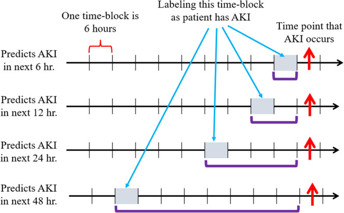
AKI labeling for different time periods prediction

Experimental Design

Figures 4 and 5 show seven main experiment settings performed on the ML in AKI risk prediction for model performance evaluation. The first three experiments (Fig. 4a–c) are local learning trained by three individual local datasets. The fourth experiment (Fig. 4d) is centralized learning trained by a single global dataset including all three local datasets. The last three experiments (Fig. 5e-g) are FL with three different aggregation processes, including pure FedAvg, neural network weight averaging with local dataset size weighting (Weighted FedAvg), and the proposed Non-IID (Weighted) FedAvg which includes non-IID combined with FedAvg and non-IID combined with Weighted FedAvg. A three-layered simple neural network for local learning, centralized learning, and FL is used to collect the experimental results.

Fig. 4.

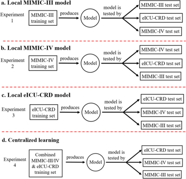
Local learning and centralized learning experiments. Sub-panels (a), (b), and (c) illustrate local learning experiments conducted using the MIMIC-III, MIMIC-IV, and eICU-CRD training sets, respectively. Sub-panel (d) presents a centralized learning experiment that utilizes a combined global dataset aggregated from all the local training sets

Fig. 5.

Federated learning experiments (this figure does not include another two FL comparison methods: FedProx [10] and Mime Lite [11]). Sub-panel (e) presents the Pure FedAvg approach, sub-panel (f) shows the Weighted FedAvg method, and sub-panel (g) depicts the proposed Non-IID (Weighted) FedAvg 

Results

This section presents the experimental results of the comparison between our non-IID estimation algorithm and other non-IID estimation algorithms, how each feature contributes to non-IID degree, the relationship between non-IID degree and testing error of several ML models, and the performance of non-IID FL. Algorithms were written in Python, and the compared FL methods, FedProx [10] and Mime Lite [11], were functions in the TensorFlow Federated API. Codes are executed on a workstation equipped with an Intel(R) Xeon(R) W-2275 @ 3.30 GHz CPU, 128 GB memory, and a NVIDIA Quadro RTX 6000 graphics card.

Performance Comparison of Non-IID Estimation Algorithms

Figure 6 presents the non-IID degree variations of the proposed algorithm and the other three previous methods under different data sampling percentages. In each subfigure, $\text{x}$-axis is the non-IID degree value and $\text{y}$-axis is the sampling percentage of the data from the original dataset. Each sample point in the figure means the non-IID degree value between some specific dataset and the comparative dataset under corresponding sampling percentage. We conducted the repeated dataset comparisons by randomly sampling from both datasets. For example, when the sampling percentage was 80%, we compared the same two datasets five times, each time randomly sampling 80% of the data from both datasets. 

Fig. 6.

Comparison of non-IID estimation methods. Each subfigure showed the non-IID degree variations under different data sampling percentages, where the subfigure title is computational time, x-axis is non-IID degree, and y-axis is the sampling percentage of data from the original dataset

Note that the 40% data of the eICU-CRD dataset is extracted to pre-train a fixed encoder model in Li et al.’s [36] proposed algorithm. Therefore, for the consistency of each experiment, we use 60% data of the eICU-CRD dataset for subsequent algorithm performance comparisons. Three datasets with the abbreviation m3, m4, and e_0.6 are referred to MIMIC-III, MIMIC-IV, and 60% eICU-CRD, respectively. From the aspect of computation time, the proposed non-IID estimation method computes the non-IID degree efficiently based on the statistics of each local dataset, while the other three algorithms must train a neural network model to obtain the non-IID degree. Their computation time is obviously greater than the proposed algorithm. From the aspect of non-IID degree variations, the proposed algorithm always has a normalized non-IID degree within 0 and 1, while the other three algorithms may have an unexpected large value.

Importantly, the proposed non-IID degree estimation algorithm has the smallest variation in predicted non-IID degree under different sampling percentages as compared to the other three algorithms.

Figure 7 shows the feasibility of applying the proposed non-IID estimation method to the mixed dataset. Here, we simplify the comparison by adopting only the MIMIC-IV dataset as the comparative dataset. The abbreviation m43 refers to the mixed dataset sampled evenly from m4 and m3 separately, while the abbreviation m4e refers to the mixed dataset sampled evenly from m4 and 60% eICU-CRD separately. Again, the quantified non-IID degree between the MIMIC-IV dataset and the mixed dataset m43 was coincidentally located between that of two datasets m4 and m3, while the quantified non-IID degree between the MIMIC-IV dataset and the mixed dataset m4e_0.6 was located between that of two datasets m4 and e_0.6. All the experimental results demonstrate that our non-IID estimation method is efficient and robust under different mixed datasets.

Fig. 7.

Comparison of non-IID estimation methods on mixed datasets. Each subfigure showed the non-IID degree variations under different data sampling percentages, where the x-axis is non-IID degree and y-axis is the sampling percentage of data from the original dataset

Table 2 presents the performance comparison of 4 non-IID estimation algorithms. In our experiment, we conducted 10 sampling percentages (random sampling data percentage range from 10 to 100%, with 10% as the step value), and repeated the dataset comparison 5 times for each sampling percentage (see the subfigures in Fig. 6 as the example). We have three datasets in the experiment; for a selected dataset, the dataset is compared to itself and also with other two datasets to quantify within-dataset and between dataset non-IID degree. We demonstrate that our method outperforms the other three methods in the tested evaluation metrics. For the separability metric, we show that our method has the highest data distribution separability and that the neural network weight comparison method has the lowest data distribution separability. For variability, our method has the lowest non-IID variability, showing the least variation between random samples, while the neural network weight comparison method has the highest non-IID measurement inconsistency. Finally, our method has the lowest computation time; this is expected because we did not train a model to calculate the non-IID degree between datasets.

Table 2.

Comparison of non-IID estimation algorithms

	Variability	Separability	Computational time (min.)
Performance evaluation	Averaged value [MIMIC-III’s value, MIMIC-IV’s value, eICU-CRD 40%’s value]
Our method	0.011 [0.012, 0.014, 0.008]	0.998 [0.998, 1, 0.995]	0.8 [0.6, 0.7, 1.0]
He et al. [21]	0.337 [0.155, 0.737, 0.120]	0.767 [0.808, 0.817, 0.676]	368.5 [344.7, 417.0, 343.8]
Li et al. [22]	0.105 [0.121, 0.102, 0.093]	0.795 [0.790, 0.930, 0.666]	17.4 [16.7, 18.7, 16.9]
Zhao et al. [23]	0.338 [0.184, 0.289, 0.541]	0.650 [0.673, 0.713, 0.564]	2161.0 [2094.4, 2166.9, 2221.6]

Analyzing Each Feature’s Contribution to Non-IID Degree for Better Non-IID Degree Interpretability

We conducted an experiment to investigate how each feature contributes to the estimated non-IID degree to interpret the calculated non-IID degree from our proposed method.

Figure 8 presents the feature contributions of non-IID values between datasets. From the figure, blood pH and anion gap were the two most frequent numerical features with the highest non-IID values, suggesting they were the most influential numerical features in non-IID estimation. Table 3 confirmed this observation by showing categorical and numerical features’ statistical values computed by statistical hypothesis testing (Welch’s t-test and Pearson’s chi-squared test) and effect size methods (Cohen’s d and Cramér’s V) that our non-IID estimation method is based on. In the table, the p values of statistical hypothesis testing indicated whether the feature distributions between two datasets were statistically different, and the higher effect size values indicated higher feature distribution difference between two datasets. For example, (1) the blood pH in the comparison of MIMIC-III and MIMIC-IV showed the highest non-IID contribution among numerical features in Fig. 8, and it also has the highest absolute Cohen’s d in Table 3. (2) The demographics feature like gender, its consistent statistical significance, and relatively high non-IID contribution suggests potential systematic differences in gender representation across datasets. This could lead to biased model performance across different gender groups when applying FL.

Fig. 8.

The feature contributions for non-IID degree

Table 3.

Data distribution comparison for categorical and numerical variables

	MIMIC-III vs. MIMIC-IV	MIMIC-III vs. eICU-CRD	MIMIC-IV vs. eICU-CRD
2 categorical variables	$\mathit{p}$ values of Pearson’s chi-squared test & effect sizes of Cramér’s $\mathit{V}$ value
AKI label	***, +	***, +	***, +
Gender	***, +	***, +	***, +
17 numerical variables	$\mathit{p}$ values of Welch’s $\mathit{t}$-test & effect sizes of absolute Cohen’s $\mathit{d}$ value
Age	⁑, +	***, +	***, +
Potassium	***, +	***, +	***, +  +
Mean corpuscular volume (MCV)	***, +  +	***, +	***, +
Sodium	⁑, +	*, +	⁑, +
Total calcium	***, +	***, +	***, +
Phosphate	***, +	***, +	***, +
Magnesium	***, +	***, +	***, +  +
International normalized ratio (INR)	*, +	***, +	***, +
Red blood cell distribution width (RDW)	***, +	***, +	***, +
Anion gap	***, +	***, +  +  +  +	***, +  +  +  +
Prothrombin time (PT)	***, +	***, +	***, +
Blood pH	***, +  +  +	***, +	***, +  +  +  +
Blood urea nitrogen (BUN)	***, +	***, +	***, +
Lactate	***, +	⁑, +	***, +
Creatinine	***, +	***, +	***, +
Total bilirubin	***, +	***, +	***, +
Partial thromboplastin time (PTT)	***, +	***, +	***, +

⁑$p\ge 0.05$, *$p<0.05$, **$p<0.01$, ***$p<0.001$, + $0<V\le 0.2$, +  + $0.2<V\le 0.5$, +  +  + $0.5<V\le 0.8$, +  +  +  + $0.8<V$, + $0<|d|\le 0.2$,  +  + $0.2<|d|\le 0.5$, +  +  + $0.5<|d|\le 0.8$, +  +  +  + $0.8<|d$

This visualization of each feature’s contribution toward non-IID value suggests that it would be possible to reduce data distribution differences between datasets by removing features with higher non-IID value contributions or implement fairness awareness techniques to achieve better model robustness in FL.

Relationship Between Non-IID Degree and Test Error

Figure 9 shows the relationship between non-IID degree and model testing error. The experiment obtains the model trained from the MIMIC-IV dataset and then applies the trained model to different datasets to measure the testing error through eight ML model architectures, including the simple neural network, 1D CNN, simple recurrent neural network (RNN), long short-term memory (LSTM) [48], eXtreme Gradient Boosting (XGBoost) [49], decision tree, random forests, and support vector machine models. The testing datasets used consist of MIMIC-IV testing set (m4 ts), MIMIC-III testing set (m3 ts), eICU-CRD testing set (e ts), mixed data from MIMIC-IV and MIMIC-III testing sets (m43 ts), and mixed data from MIMIC-IV and eICU-CRD testing sets (m4e ts). We observe that as non-IID degree between training and evaluation datasets increases, the testing error also increases. All subfigures in Fig. 9 show there is a positive correlation relationship between non-IID degree and testing error for all eight different ML model architectures.

Fig. 9.

The positive correlation relationship between estimated non-IID degree and model testing error using MIMIC-IV as training dataset

Our result validates the findings in He et al. [21] who showed their non-IID degree positively related to testing error using image datasets, and also Miller et al. [50] who examined the relationship between in-distribution (the testing set is sampled from same distribution as the training set) model performance and out-of-distribution (the training set and the testing set are not identically distributed) model performance. Miller et al. [50] demonstrated that models with higher in-distribution performance tends to have higher out-of-distribution performance on variants of CIFAR-10 and ImageNet datasets; they also showed that the data covariance change from distribution shift could affect the correlations between in-distribution and out-of-distribution performances.

Non-IID Federated Learning

Table 4 shows the testing accuracy comparison by directly applying three different learning methods, including centralized learning, local learning, and FL, on each dataset. Generally, people feel that centralized learning with all the datasets leads to the best model performance. In our experiments on the three datasets, our models such as Non-IID FedAvg can achieve test accuracies of 79.04%, 74.63%, and 85.87% for each test dataset separately. Local learning based on the MIMIC-IV dataset has the largest variance from 48.59 to 85.37%, while local learning based on the other two datasets have the similar test accuracy compared to centralized learning.

Table 4.

Performance comparison of different learning methods (with the same NN architecture and hyperparameters)

Datasets	MIMIC-III	MIMIC-IV	eICU-CRD	Average accuracy
Learning methods
Centralized learning	77.06%	72.42%	85.36%	78.28%
Local learning using MIMIC-III	77.15%	73.31%	85.29%	78.58%
Local learning using MIMIC-IV	67.80%	83.02%	48.59%	66.47%
Local learning using eICU-CRD	78.04%	72.96%	85.37%	78.79%
FedAvg [8]	72.86%	77.48%	83.21%	77.85%
Weighted FedAvg [8]	72.68%	77.21%	83.22%	77.70%
Weighted FedProx [10]	58.56%	60.44%	66.79%	61.93%
Weighted Mime Lite [11]	51.84%	52.58%	55.51%	53.21%
Non-IID Weighted FedAvg	79.04%	74.63%	85.87%	79.85%
Non-IID FedAvg	79.03%	75.83%	84.44%	79.77%

For FL, pure FedAvg and weighted FedAvg algorithms have average testing accuracy of 77.85% and 77.70%, slightly lower than that of centralized learning. And other two FL algorithms, the Weighted FedProx [10] and Weighted Mime Lite [11] average 61.93% and 53.21% accuracy. Our proposed non-IID FL algorithm has the highest average accuracy among all algorithms tested, which suggests inclusion of more data sets does not always guarantee better model performance. By quantifying non-IID degree, the robustness of ML algorithms can be improved.

Our FL results also show that we can simultaneously improve models’ performance and robustness such that there seems to be no noticeable tradeoff between the two as others [11] have suggested. This validates the idea in Yang et al. [51] who suggested that the tradeoff between model robustness and prediction accuracy in deep learning is not inherent. We hypothesize that this is because analyses of the robustness-accuracy tradeoff were mainly conducted in local learning setting. In FL, although global model is not directly trained by local dataset, it is created by the aggregation of local models which contributes the information of local datasets indirectly to the global model through model parameters.

Conclusion

Summary of This Study

This study proposes a new non-IID estimation method to measure the difference in underlying data distributions between local tabular EHR datasets, three metrics to evaluate the performance of previous non-IID estimation methods, and a non-IID FL algorithm. Without the sharing of raw data across data silos, the proposed method can estimate how different separate datasets are, using statistical analysis of the datasets. The estimated non-IID degree can be then used to predict the impact of each dataset on the overall FL performance. We evaluate the algorithm performance through a series of experiments to discuss the relationship between non-IID degree and testing accuracy. We also demonstrate the efficiency, robustness, and interpretability of the proposed non-IID estimation method compared to other model-based non-IID degree calculations. Finally, integrating the non-IID issue into AKI risk prediction concludes that, in some cases, centralized learning with more training data could potentially lead to lower model performance if data heterogeneity is not accounted for.

Future Directions

There are several promising research directions to further enhance and expand our work:

1. Dataset selection framework for FL: Our non-IID estimation method could be enhanced to serve as a dataset selection framework for FL, helping determine which datasets would be beneficial or detrimental to include based on their non-IID degrees. This could involve developing theoretical frameworks to establish optimal non-IID degree thresholds for dataset inclusion and investigating how different types of distribution shifts impact model performance differently.

2. Integration of SDoH into Non-IID estimation: Integrating SDoH into non-IID estimation could provide crucial insights into health disparities and their impact on model performance. A SDoH-aware non-IID estimation approach could help quantify how socioeconomic factors, demographics, and healthcare access patterns contribute to distribution shifts between institutions. This could inform more equitable dataset selection strategies for FL training and help identify potential sources of bias in model predictions.

3. Broad applicability of non-IID estimation method across diverse domains: Our non-IID estimation method has potential applications beyond healthcare datasets, such as in finance, education, and retail domains, where data distribution can exhibit significant heterogeneity due to demographic diversity, socioeconomic or geographic disparities, or context-specific factors. Technically, our method does not require substantial changes to address tabular datasets in other domains. The proposed framework quantifies non-IID degree based on attribute skew and label distribution skew, which are generalizable across domains. For example: In finance, attribute skew may involve income and transaction patterns, while label skew may involve loan default outcomes. In education, attribute skew could involve student demographics, while label skew might reflect academic performance. By adjusting the input features and labels to align with domain-specific characteristics, our method can be applied to tabular datasets in other domains.

Author Contribution

K.Y.C. conducted the experiments and drafted the manuscript. C.R.S. and Z.Y.S. co-supervised the project and conceived the original idea. Y.Y.T. and W.I.B. contributed to manuscript writing and data interpretation. C.Y. Chang helped experimental implementations and data preprocessing. C.Y. Chou provided clinical expertise in acute kidney injury. C.R.S., Z.Y.S., Y.Y.T., W.I.B., and J.P.T. reviewed and provided critical feedback for the manuscript. All authors approved the final manuscript.

Funding

This work was supported by the National Science and Technology Council of Taiwan under Grant MOST 111–2321-B-468–001 (K.Y.C., Z.Y.S., C.Y. Chang, Y.Y.T., J.P.T.). It was partially funded by Shumaker Endowment for Biomedical Informatics (K.Y.C., C.R.S.) and the National Institutes of Health under grant 5T32LM012410 (W.I.B.).

Data Availability

The data used in this study are available in the following publicly accessible repositories: Medical Information Mart for Intensive Care (MIMIC)-III database (https://physionet.org/content/mimiciii/1.4/), MIMIC-IV database (https://physionet.org/content/mimiciv/3.1/), and eICU Collaborative Research Database (eICU-CRD) (https://physionet.org/content/eicu-crd/2.0/). Access to these databases requires completion of a training course and acceptance of a data use agreement through PhysioNet. Due to the sensitive nature of the healthcare data, researchers must be credentialed users to access the databases.

Declarations

Competing Interests

The authors declare no competing interests.

References

- 1.Rajendran S, Xu Z, Pan W, Ghosh A, Wang F (2023) Data heterogeneity in federated learning with electronic health records: case studies of risk prediction for acute kidney injury and sepsis diseases in critical care. PLOS Digital Health 2(3):e0000117. 10.1371/journal.pdig.0000117 [DOI] [PMC free article] [PubMed] [Google Scholar]
- 2.Parikh RB, Teeple S, Navathe AS (2019) Addressing bias in artificial intelligence in health care. JAMA 322(24):2377–2378. 10.1001/jama.2019.18058 [DOI] [PubMed] [Google Scholar]
- 3.Mehrabi N, Morstatter F, Saxena N, Lerman K, Galstyan A (2021) A survey on bias and fairness in machine learning. ACM computing surveys (CSUR) 54(6):1–35. 10.1145/3457607 [Google Scholar]
- 4.Giovanola B, Tiribelli S (2023) Beyond bias and discrimination: redefining the AI ethics principle of fairness in healthcare machine-learning algorithms. AI & Soc 38(2):549–563. 10.1007/s00146-022-01455-6 [DOI] [PMC free article] [PubMed] [Google Scholar]
- 5.Chunara R et al (2024) Social determinants of health: the need for data science methods and capacity. The Lancet Digital Health 6(4):e235–e237. 10.1016/S2589-7500(24)00022-0 [DOI] [PMC free article] [PubMed] [Google Scholar]
- 6.Kino S et al (2021) A scoping review on the use of machine learning in research on social determinants of health: trends and research prospects. SSM-population Health 15:100836. 10.1016/j.ssmph.2021.100836 [DOI] [PMC free article] [PubMed] [Google Scholar]
- 7.Mittermaier M, Raza MM, Kvedar JC (2023) Bias in AI-based models for medical applications: challenges and mitigation strategies. NPJ Digit Med 6(1):113. 10.1038/s41746-023-00858-z [DOI] [PMC free article] [PubMed] [Google Scholar]
- 8.Prayitno et al (2021) A systematic review of federated learning in the healthcare area: from the perspective of data properties and applications. Appl Sci 11(23):11191. 10.3390/app112311191 [Google Scholar]
- 9.McMahan B, Moore E, Ramage D, Hampson S, y Arcas BA (2017) Communication-efficient learning of deep networks from decentralized data. In: Artificial intelligence and statistics. PMLR, pp 1273–1282
- 10.Li T, Sahu AK, Zaheer M, Sanjabi M, Talwalkar A, Smith V (2020) Federated optimization in heterogeneous networks. Proc Mach Learn Syst 2:429–450 [Google Scholar]
- 11.Karimireddy SP, Jaggi M, Kale S, Mohri M, Reddi SJ, Stich SU, Suresh AT (2020) Mime: mimicking centralized stochastic algorithms in federated learning. arXiv preprint arXiv:2008.03606 . Accessed 16 Feb 2025
- 12.Johnson AE et al (2016) MIMIC-III, a freely accessible critical care database. Sci Data 3(1):1–9. 10.1038/sdata.2016.35 [DOI] [PMC free article] [PubMed] [Google Scholar]
- 13.Johnson AE et al (2023) MIMIC-IV, a freely accessible electronic health record dataset. Sci Data 10(1):1. 10.1038/s41597-022-01899-x [DOI] [PMC free article] [PubMed] [Google Scholar]
- 14.Pollard TJ, Johnson AE, Raffa JD, Celi LA, Mark RG, Badawi O (2018) The eICU Collaborative Research Database, a freely available multi-center database for critical care research. Sci Data 5(1):1–13. 10.1038/sdata.2018.178 [DOI] [PMC free article] [PubMed] [Google Scholar]
- 15.Nouretdinov I, Vovk V, Vyugin M, Gammerman A (2001) Pattern recognition and density estimation under the general IID assumption. International Conference on Computational Learning Theory. Springer, pp 337–353 [Google Scholar]
- 16.Vapnik VN (1999) An overview of statistical learning theory. IEEE Trans Neural Networks 10(5):988–999. 10.1109/72.788640 [DOI] [PubMed] [Google Scholar]
- 17.Yang Q, Liu Y, Chen T, Tong Y (2019) Federated machine learning: concept and applications. ACM Trans Intell Syst Technol 10(2):1–19. 10.1145/3298981 [Google Scholar]
- 18.Ontañón S (2020) An overview of distance and similarity functions for structured data. Artif Intell Rev 53(7):5309–5351. 10.1007/s10462-020-09821-w [Google Scholar]
- 19.Levy A, Shalom BR, Chalamish M (2024) A guide to similarity measures. arXiv preprint arXiv:2408.07706 . Accessed 16 Feb 2025
- 20.Menéndez ML, Pardo J, Pardo L, Pardo M (1997) The jensen-shannon divergence. J Franklin Inst 334(2):307–318. 10.1016/S0016-0032(96)00063-4 [Google Scholar]
- 21.He Y, Shen Z, Cui P (2021) Towards non-IID image classification: a dataset and baselines. Pattern Recogn 110:107383. 10.1016/j.patcog.2020.107383 [Google Scholar]
- 22.Li A, et al (2021) Lotteryfl: empower edge intelligence with personalized and communication-efficient federated learning. In: 2021 IEEE/ACM Symposium on Edge Computing (SEC). IEEE, pp 68–79. 10.1145/3453142.3492909
- 23.Zhao Y, Li M, Lai L, Suda N, Civin D, Chandra V (2018) Federated learning with non-IID data. arXiv preprint arXiv:1806.00582 . Accessed 16 Feb 2025
- 24.Lu Z, Pan H, Dai Y, Si X, Zhang Y (2024) Federated learning with non-IID data: a survey. IEEE Internet Things J. 10.1109/JIOT.2024.3376548
- 25.Yun WJ et al (2023) SlimFL: federated learning with superposition coding over slimmable neural networks. IEEE/ACM Trans Netw 31(6):2499–2514. 10.1109/TNET.2022.3231864 [Google Scholar]
- 26.Luo Y, Liu X, Xiu J (2021) Energy-efficient clustering to address data heterogeneity in federated learning. In: ICC 2021-IEEE International Conference on Communications. IEEE, pp 1–6. 10.1109/ICC42927.2021.9500901
- 27.Zhang W, Wang X, Zhou P, Wu W, Zhang X (2021) Client selection for federated learning with non-IID data in mobile edge computing. IEEE Access 9:24462–24474. 10.1109/ACCESS.2021.3056919 [Google Scholar]
- 28.Lee J, Ko H, Seo S, Pack S (2022) Data distribution-aware online client selection algorithm for federated learning in heterogeneous networks. IEEE Trans Veh Technol 72(1):1127–1136. 10.1109/TVT.2022.3205307 [Google Scholar]
- 29.Duan M, et al (2021) Fedgroup: efficient federated learning via decomposed similarity-based clustering. In: 2021 IEEE Intl Conf on Parallel & Distributed Processing with Applications, Big Data & Cloud Computing, Sustainable Computing & Communications, Social Computing & Networking (ISPA/BDCloud/SocialCom/SustainCom). IEEE, pp 228–237. 10.1109/ISPA-BDCloud-SocialCom-SustainCom52081.2021.00042
- 30.Kim H, Kim B, Kim Y, You C, Park H (2023) K-FL: Kalman filter-based clustering federated learning method. IEEE Access 11:36097–36105. 10.1109/ACCESS.2023.3264584 [Google Scholar]
- 31.Zhu H, Xu J, Liu S, Jin Y (2021) Federated learning on non-IID data: a survey. Neurocomputing 465:371–390. 10.1016/j.neucom.2021.07.098 [Google Scholar]
- 32.Ma X, Zhu J, Lin Z, Chen S, Qin Y (2022) A state-of-the-art survey on solving non-IID data in federated learning. Futur Gener Comput Syst 135:244–258. 10.1016/j.future.2022.05.003 [Google Scholar]
- 33.Maliakel PJ, Ilager S, Brandic I (2024) FLIGAN: enhancing federated learning with incomplete data using GAN. In: Proceedings of the 7th International Workshop on Edge Systems, Analytics and Networking, 2024, pp 1–6. 10.1145/3642968.3654813
- 34.Liu J, Zhao Z, Luo X, Li P, Min G, Li H (2024) SlaugFL: efficient edge federated learning with selective GAN-based data augmentation. IEEE Transactions on Mobile Computing. 10.1109/TMC.2024.33975
- 35.Zhao L, Huang J (2023) A distribution information sharing federated learning approach for medical image data. Complex Intell Syst 9(5):5625–5636. 10.1007/s40747-023-01035-1 [DOI] [PMC free article] [PubMed] [Google Scholar]
- 36.Long G, Xie M, Shen T, Zhou T, Wang X, Jiang J (2023) Multi-center federated learning: clients clustering for better personalization. World Wide Web 26(1):481–500. 10.1007/s11280-022-01046-x [Google Scholar]
- 37.Li Q, He B, Song D (2021) Model-contrastive federated learning. In: Proceedings of the IEEE/CVF conference on computer vision and pattern recognition, pp 10713–10722. 10.1109/CVPR46437.2021.01057
- 38.Chen R, et al (2023) Workie-talkie: accelerating federated learning by overlapping computing and communications via contrastive regularization. In Proceedings of the IEEE/CVF international conference on computer vision, pp 16999–17009. 10.1109/ICCV51070.2023.01559
- 39.Yamamoto F, Ozawa S, Wang L (2022) eFL-Boost: Efficient federated learning for gradient boosting decision trees. IEEE Access 10:43954–43963. 10.1109/ACCESS.2022.3169502 [Google Scholar]
- 40.Jiang J, Jiang H, Ma Y, Liu X, Fan C (2024) Low-parameter federated learning with large language models," in International Conference on Web Information Systems and Applications. Springer, pp 319–330. 10.1007/978-981-97-7707-5_28
- 41.Ju L, Zhang T, Toor S, Hellander A (2024) Accelerating fair federated learning: adaptive federated Adam. IEEE Transactions on Machine Learning in Communications and Networking. 10.1109/TMLCN.2024.3423648
- 42.Wu X, Huang F, Hu Z, Huang H (2023) Faster adaptive federated learning. Proc Int AAAI Conf Artif Intell 37(9):10379–10387. 10.1609/aaai.v37i9.26235 [Google Scholar]
- 43.Guo W, Zhuang F, Zhang X, Tong Y, Dong J (2024) A comprehensive survey of federated transfer learning: challenges, methods and applications. Front Comp Sci 18(6):186356. 10.1007/s11704-024-40065-x [Google Scholar]
- 44.Pinto Neto EC, Sadeghi S, Zhang X (2023) Dadkhah S (2023) Federated reinforcement learning in IoT: applications, opportunities and open challenges. Appl Sci 13(11):6497. 10.3390/app13116497 [Google Scholar]
- 45.Lin S, Yang G, Zhang J (2020) A collaborative learning framework via federated meta-learning," in 2020 IEEE 40th International Conference on Distributed Computing Systems (ICDCS). IEEE, pp 289–299. 10.1109/ICDCS47774.2020.00032
- 46.Levin A, Stevens PE (2014) Summary of KDIGO 2012 CKD Guideline: behind the scenes, need for guidance, and a framework for moving forward. Kidney Int 85(1):49–61. 10.1038/ki.2013.444 [DOI] [PubMed] [Google Scholar]
- 47.White IR, Royston P, Wood AM (2011) Multiple imputation using chained equations: issues and guidance for practice. Stat Med 30(4):377–399. 10.1002/sim.4067 [DOI] [PubMed] [Google Scholar]
- 48.Hochreiter S, Schmidhuber J (1997) Long short-term memory. Neural Computation MIT-Press. 10.1162/neco.1997.9.8.1735 [DOI] [PubMed]
- 49.Chen T, Guestrin C (2016) Xgboost: a scalable tree boosting system. In: Proceedings of the 22nd acm sigkdd international conference on knowledge discovery and data mining, pp 785–794. 10.1145/2939672.2939785
- 50.Miller JP, et al (2021) Accuracy on the line: on the strong correlation between out-of-distribution and in-distribution generalization," in International Conference on Machine Learning. PMLR, pp 7721–7735
- 51.Yang Y-Y, Rashtchian C, Zhang H, Salakhutdinov RR, Chaudhuri K (2020) A closer look at accuracy vs. robustness. Adv Neural Inf Process Syst 33:8588–8601 [Google Scholar]
Associated Data
This section collects any data citations, data availability statements, or supplementary materials included in this article.
Data Availability Statement