Design and Nonlinear Modeling of a Modular Cable-Driven Soft Robotic Arm

Abstract

We propose a novel multi-section cable-driven soft robotic arm inspired by octopus tentacles along with a new modeling approach. Each section of the modular manipulator is made of a soft tubing backbone, a soft silicon arm body, and two rigid endcaps, which connect adjacent sections and decouple the actuation cables of different sections. The soft robotic arm is made with casting after the rigid endcaps are 3D-printed, achieving low-cost and convenient fabrication. To capture the nonlinear effect of cables pushing into the soft silicon arm body, which results from the absence of intermediate rigid cable guides for higher compliance, an analytical static model is developed to describe the relationship between the bending curvature and the cable lengths. The proposed model shows superior prediction performance in experiments over that of a baseline model, especially under large bending conditions. Based on the nonlinear static model, a kinematic model of a multi-section arm is further developed and used to derive a motion planning algorithm. Experiments show that the proposed soft arm has high flexibility and a large workspace, and the tracking errors under the algorithm based on the proposed modeling approach are up to 52% smaller than those with the algorithm derived from the baseline model.

I. Introduction

Soft robotic manipulators have been widely proposed and developed for their various advantages, such as safe human-machine interactions, robustness, and flexibility [1], [2]. Compared with their fully rigid counterparts, soft manipulators can utilize the softness of their body structures to adapt to external collisions and constraints and mitigate risks to humans, while being able to accomplish manipulation tasks [3], [4]. The advantages of soft manipulators make them competitive candidates for applications involving the handling of delicate and complex objects, as in fruit harvesting and medical surgeries [5]–[7].

Multiple structures and actuation methods have been developed for building soft robotics arms to achieve efficient deformation. For example, fluid-driven methods are widely used for soft actuators, where fluid pressures inside chambers are modulated to generate elastic deformation [8], [9]. Soft actuators have also been constructed with other mechanisms including smart materials [10]. In particular, the cable-driven method is popular thanks to its simplicity and high force-to-weight ratio [11], [12], where embedded eccentric cables driven by motors deliver torques to achieve deformation of the soft body.

To control the deformation of the soft arm effectively, models that capture the relationship between the actuation space and the task space of the robotic arm have been developed. The modeling is generally complex and often dependent on robot designs and actuation methods. Models for fluid-driven actuators are often built based on static and dynamic analysis [13]. For simple cable-driven actuators, models have been built based on geometry relationships [14]. Static models for tendon-driven manipulators have also been proposed to analyze the deformation of the elastic tendons [15]. In addition, models have been reported for the coupling and decoupling cable system of multi-section soft manipulators [14], [16]. Piecewise constant curvature (PCC) models are widely utilized due to their simplicity [14], while other models, such as finite element method (FEM) models and Cosserat rod models are proposed with better accuracy but higher complexity [17], [18]. In addition, piecewise constant strain (PCS) and geometric variable strain models have been proposed that allow more general settings [19].

Many biological structures and mechanisms have inspired the design of robotic systems, and conversely, the development of robots has provided bio-physical models for understanding biomechanics [20]. In this study, inspired by the longitudinal muscles in the octopus tentacles, we propose a novel decoupled modular cable-driven soft robotic arm fabricated with a integrated molding technique. We further develop a novel analytical static model that considers the prominent nonlinear effect of the cable pushing into the soft body of the robotic arm. To our best knowledge, this is the first effort in explicitly modeling the transverse deformation effect in soft cable-driven actuators, which extensively exists and potentially significantly influence the actuation length of the cable.

Specifically, a novel composite structure of a single section of the arm consists of multiple parts: flexible backbone, soft silicone body, multi-purpose rigid caps, and embedded coil-reinforced cable guides with high compliance (Fig. 1B). A piece of soft tubing is selected as the backbone to constrain the axial deformation. Two rigid endcaps are attached to the ends of the backbone, which act as connectors between sections and anchor points for cables. The soft silicone body is made by casting with three specially-designed evenly embedded fiber-reinforced cable guides that protect the soft body while maintaining high compliance. Actuation cables in the cable guides provide contraction forces like longitudinal muscles while the cavities are able to reduce the bending stiffness of the soft arm.

Figure 1. Structures of the soft robotic arm.

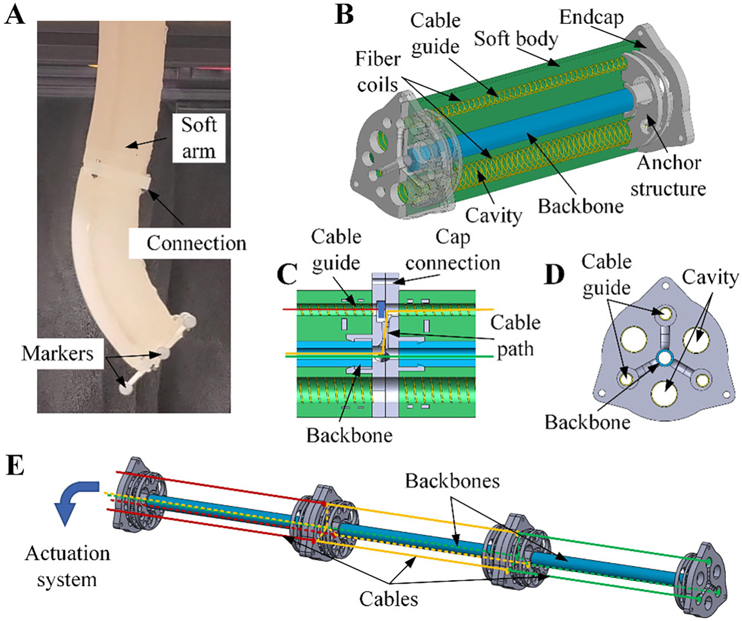
(A). A two-section modular soft robotic arm. (B). The structure for one section of the robotic arm. (C). Connection of two endcaps. (D) One endcap at the tip side of the section. (E). Cable paths for different sections of the soft robotic arm.

The soft modular multi-section robotic arm consists of identical sections with an embedded cable system. The unique actuation decoupling mechanism is achieved by the connection of the multi-propose endcaps, which generate pathways between the cable guides and the backbone tubing (Fig. 1C–D). The actuation cables, with their one end fixed on the endcap, pass through the cable guides in one section and go into the backbone tubing through the pathways before they are attached to the corresponding driving motors, which presents a convenient routing scheme thank to the endcap design of the actuation decoupling mechanism (Fig. 1E). When one section of the arm has a bending deformation, its backbone maintains a nearly constant length, ensuring the lengths of the actuation cables for other sections do not passively change. During the bending motion of the multi-section robotic arm, the backbone tubing protects the actuation system for other sections, separating the deformation of one section from the change of cable lengths of other sections, and thus achieving actuation decoupling between different sections of the robotic arm.

II. Materials and Methods

Each section of the modular soft robotic arm was fabricated separately by using integrated molding and then assembled together. The endcaps and the molds for each section were fabricated with a 3D printer (Objet Connex 350) using rigid material (Objet Vero White). After the molds were assembled with flexible tubing (Clear Masterkleer Soft PVC Plastic Tubing, McMaster-Carr), which acted as the backbone, a silicone material (Ecoflex 00–10, Smooth-On) was utilized to cast the soft body of each section, before different sections and the cable system were assembled. More details on the fabrication of the soft robotic arm and on the experimental setups are given in Supplementary Materials.

III. Modeling of the Soft Robotic Arm

The model for the multi-section soft robotic arm is separated into two parts: a static model for a single section, which maps the actuation cable lengths to the bending configuration of one section; and another model that characterizes the relationship between the bending configurations for all sections and the task space variables (in particular, the end position of the arm). A parameter list is provided in the Supplementary Materials (S2) for the convenience of readers.

A. Static Model of a Section Driven by a Single Cable

The static model for a single section of the robotic arm is built based on the analysis of its bending deformation. Before studying a section with multiple actuation cables, we consider the case with a single actuating cable and analyze an arbitrary bending configuration (Fig. 2A). The cable and the support of the section provide external forces. To simplify the static analysis, several assumptions are made: (A1) The backbone (dash line) of the soft section has a constant length. (A2) The backbone and the cable (red line) have constant curvatures. (A3) The backbone has bending deformations within one single plane. (A4) The friction between the cables and the soft body of the arm is negligible. (A5) The soft section of the arm has a linear bending stiffness with no hysteresis. (A6) The cables have no slacks.

Figure 2. Modeling of one section of the arm driven by a single cable.

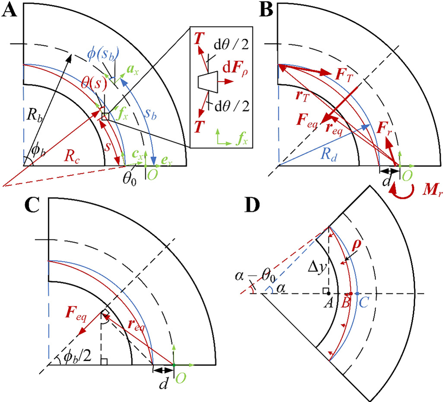
(A). Bending configuration for one section driven by a single cable. (B). External forces and moments applied by the cable to the soft section. (C) The total transverse force applied by the cable and its arm. (D). Actuation cable considering transverse deformation (red) and without transverse deformation (blue).

Refer to Fig. 2A. Let $s_b$ (subscript “$b$” for “backbone”) be the arclength parameter for the backbone. The bending angle $\varphi \left(s_b\right)$ of the section at a given point with an arclength $s_b$ is defined as the angle of rotation between the two local frames at the base, $\mathit{e}=\left({\mathit{e}}_x,{\mathit{e}}_y\right)$, and at the point with $s_b$ on the backbone, $\mathit{a}=\left({\mathit{a}}_x,{\mathit{a}}_y\right)$, and can be described as:

$$\varphi \left(s_b\right)=\frac{s_b}{R_b}$$ (1)

where $R_b$ is the radius of the backbone curvature. The curvature of the backbone, ${\kappa }_b$, is written as: ${\kappa }_b=\frac{\mathrm{d}\varphi }{\mathrm{d}{s}_b}=\frac{1}{R_b}$.

The curvature ${\kappa }_c$ (subscript “$c$” for “cable”) for the cable is described similarly: ${\kappa }_c=1/R_c$, where $R_c$ is the radius of the actuation cable curvature, and $s$ is the arclength parameter for the cable. As illustrated in Fig. 2A, $\theta \left(s\right)$ is the rotation angle between the base frame $\mathit{e}$ and $\mathit{f}=\left({\mathit{f}}_x,{\mathit{f}}_y\right)$, where $\mathit{f}$ is the local frame at the point with an arclength of $s$ on the cable.

Based on the force balance (Fig. 2A), the transverse force density $\rho$ between the cable and soft body (Fig. 2D) is derived:

$$\rho =\frac{\mathrm{d}{F}_{\rho }}{\mathrm{d}s}=T{\kappa }_c$$ (2)

where $\mathrm{d}{F}_{\rho }=T\mathrm{d}\theta$, d denotes the differential operator, $T$ is the tension of the cable, $F_{\rho }$ is the transverse force between the cable and the soft body, $\theta$ is used to denote $\theta \left(s\right)$ for simplicity, the notation “d” represents differential, and the relationship $\frac{\mathrm{d}\theta }{\mathrm{d}s}={\kappa }_c$ is used in the derivation of (2).

Another assumption following the introduction of $\rho$ is made to describe a simplified interaction model between the cable and the soft body of the arm:

(A7) The maximum transverse deformation of the cable ($\left|BC\right|$ in Fig. 2D) is proportional to the transverse force density $\rho$ applied by the cable (Fig. 2D).

Next, the transverse force density vector ${\mathit{\rho }}^e$ at point $s$, viewed in the base frame $\mathit{e}$ (Fig. 2A), is calculated by using a rotation matrix $R_f^e$:

$${\mathit{\rho }}^{\mathit{e}}(\theta )=R_f^e\left[\begin{array}{c}-\rho \\ 0\end{array}\right]$$ (3)

$$R_f^e(\theta )=\left[\begin{array}{cc}\mathrm{c}\mathrm{o}\mathrm{s}\theta & -\mathrm{s}\mathrm{i}\mathrm{n}\theta \\ \mathrm{s}\mathrm{i}\mathrm{n}\theta & \mathrm{c}\mathrm{o}\mathrm{s}\theta \end{array}\right]$$ (4)

The total transverse force ${\mathit{F}}_{eq}$ (subscript “$eq$” for “equivalent total force”) between the cable and the soft body (Fig. 2B) can then be obtained by the following integration:

$${\mathit{F}}_{eq}={\int }_0^l {\mathit{\rho }}^{\mathit{e}}(\theta (s))\mathrm{d}s=T\left[\begin{array}{c}-\mathrm{s}\mathrm{i}\mathrm{n}\left({\varphi }_b-{\theta }_0\right)+\mathrm{s}\mathrm{i}\mathrm{n}{\theta }_0\\ \mathrm{c}\mathrm{o}\mathrm{s}\left({\varphi }_b-{\theta }_0\right)-\mathrm{c}\mathrm{o}\mathrm{s}{\theta }_0\end{array}\right]$$ (5)

where $l$ is the cable length in the soft section, ${\varphi }_b$ is the bending angle of the backbone at the tip, and ${\theta }_0$ is the incident angle of the cable, which is the angle between the tangent line (${\mathit{c}}_y$ axis) of the cable at the base surface and the normal (${\mathit{e}}_y$ axis) of the base surface (Fig. 2A).

The contraction force ${\mathit{F}}_T$ applied by the cable tip to the soft section (Fig. 2B) is calculated as:

$${\mathit{F}}_T=R_f^e\left({\varphi }_b-{\theta }_0\right)\cdot \left[\begin{array}{c}0\\ -T\end{array}\right]=T\left[\begin{array}{c}\mathrm{s}\mathrm{i}\mathrm{n}\left({\varphi }_b-{\theta }_0\right)\\ -\mathrm{c}\mathrm{o}\mathrm{s}\left({\varphi }_b-{\theta }_0\right)\end{array}\right]$$ (6)

From the force balance equation: ${\mathit{F}}_r+{\mathit{F}}_{eq}+{\mathit{F}}_T=0$, where ${\mathit{F}}_r$ (subscript “$r$” for “reaction”) represents the support force applied by the base support of the soft section to the soft section (Fig. 2B), one can derive:

$${\mathit{F}}_r=-{\mathit{F}}_{eq}-{\mathit{F}}_T=T\left[\begin{array}{c}-\mathrm{s}\mathrm{i}\mathrm{n}{\theta }_0\\ \mathrm{c}\mathrm{o}\mathrm{s}{\theta }_0\end{array}\right]$$ (7)

Next, the moment balance of the section is analyzed with respect to the base point $O$ (Fig. 2B). The arm ${\mathit{r}}_T$ (Fig. 2B) for ${\mathit{F}}_T$ is derived as:

$${\mathit{r}}_T=\left[\begin{array}{c}-d-2R_d{\mathrm{s}\mathrm{i}\mathrm{n}}^2\left({\varphi }_b/2\right)\\ 2R_d\mathrm{s}\mathrm{i}\mathrm{n}\left({\varphi }_b/2\right)\mathrm{c}\mathrm{o}\mathrm{s}\left({\varphi }_b/2\right)\end{array}\right]$$ (8)

where $R_d$ is the radius of the cable curvature (Fig. 2B) when the transverse deformation of the cable is not considered, $d$ is the distance between the incident point of the cable and the base point $O$ of the section.

Since ${\mathit{F}}_{eq}$ is located on the mirror-symmetric axis of the bending section (see Fig. 2C), the point of action of ${\mathit{F}}_{eq}$ is irrelevant in computing the resulting moment around point $O$; in other words, the moment is the same regardless of the point of action of ${\mathit{F}}_{eq}$. We have thus chosen the point of action as illustrated in Fig. 2C, with the associated arm vector:

$${\mathit{r}}_{eq}=\left[\begin{array}{c}-d-R_d{\mathrm{s}\mathrm{i}\mathrm{n}}^2\left({\varphi }_b/2\right)\\ R_d\mathrm{s}\mathrm{i}\mathrm{n}\left({\varphi }_b/2\right)\mathrm{c}\mathrm{o}\mathrm{s}\left({\varphi }_b/2\right)\end{array}\right]$$ (9)

From the moment balance of the section: ${\mathit{M}}_r+{\mathit{M}}_{eq}+{\mathit{M}}_T=0$, where ${\mathit{M}}_r$ denotes the support moment (Fig. 2B), ${\mathit{M}}_{eq}$ and ${\mathit{M}}_T$ are the moments generated by ${\mathit{F}}_{eq}$ and ${\mathit{F}}_T$ with respect to point $O$, respectively (Fig. 2B), and:

$${\mathit{M}}_{eq}+{\mathit{M}}_T={\mathit{r}}_{eq}\times {\mathit{F}}_{eq}+{\mathit{r}}_T\times {\mathit{F}}_T=Td\mathrm{c}\mathrm{o}\mathrm{s}{\theta }_0$$ (10)

one obtains:

$${\mathit{M}}_r=-\left({\mathit{M}}_{eq}+{\mathit{M}}_T\right)=-Td\mathrm{c}\mathrm{o}\mathrm{s}{\theta }_0$$ (11)

See the Supplemental Materials (S2) for calculation details of this concise result. Next, the incident angle of the cable ${\theta }_0$ (Fig. 2A, D) satisfies:

$$\mathrm{\Delta }y=\left(R_b-d\right)\mathrm{s}\mathrm{i}\mathrm{n}\alpha =R_c\mathrm{s}\mathrm{i}\mathrm{n}\left(\alpha -{\theta }_0\right)$$ (12)

which implies:

$${\theta }_0=\alpha -\mathrm{a}\mathrm{r}\mathrm{c}\mathrm{s}\mathrm{i}\mathrm{n}\left(\left(1-{\kappa }_{b}d\right)\frac{{\kappa }_c}{{\kappa }_b}\mathrm{s}\mathrm{i}\mathrm{n}\alpha \right)$$ (13)

where $\alpha ={\varphi }_b/2$.

Based on assumption (A7) and the geometric relationships (Fig. 2D), one can obtain:

$$\mathrm{\Delta }h=\left|BC\right|=R_d(1-\mathrm{c}\mathrm{o}\mathrm{s}\alpha )-R_c\left(1-\mathrm{c}\mathrm{o}\mathrm{s}\left(\alpha -{\theta }_0\right)\right)$$ (14)

$$\rho =K_c\mathrm{\Delta }h$$ (15)

where $∆h$ is the maximum transverse deformation of the cable, and $K_c$ is the coefficient in the simplified linear relationship between $∆h$ and $\rho$, which is influenced by physical characters of the soft arm (e.g. elasticity modulus). The value of $K_c$ is obtained via experimental calibration.

Based on assumption (A5), the relationship between the bending deformation and the external torque is derived by introducing a bending stiffness $K_b$:

$$\left|{\mathit{M}}_{eq}+{\mathit{M}}_T\right|=\left|{\mathit{M}}_r\right|=M_r=K_b{\kappa }_b$$ (16)

where $K_b{\kappa }_b$ is the internal elastic moment. The value $K_b$ is also influenced by the physical characters of the arm and calibrated by using experiments.

Finally, by using the equations (2), (11), (13)–(16), and the geometric relationships, the model for a single soft section driven by a single cable is captured by:

$$\left\{\begin{array}{c}{K}_b{\kappa }_b=Td\mathrm{c}\mathrm{o}\mathrm{s}{\theta }_0\\ {\theta }_0=\alpha -\mathrm{a}\mathrm{r}\mathrm{c}\mathrm{s}\mathrm{i}\mathrm{n}\left(\left(1-{\kappa }_{b}d\right)\frac{{\kappa }_c}{{\kappa }_b}\mathrm{s}\mathrm{i}\mathrm{n}\alpha \right)\\ T=\frac{K_c}{{\kappa }_c}\left\{\left(\frac{1}{{\kappa }_b}-d\right)(1-\mathrm{c}\mathrm{o}\mathrm{s}\alpha )-\frac{1}{{\kappa }_c}\left(1-\mathrm{c}\mathrm{o}\mathrm{s}\left(\alpha -{\theta }_0\right)\right)\right\}\\ l=R_c\left({\varphi }_b-2{\theta }_0\right)=\frac{1}{{\kappa }_c}\left(L{\kappa }_b-2{\theta }_0\right)\end{array}\right.$$ (17)

where $L$ is the length of the soft section’s backbone. In the forward mapping from actuation to the robotic arm configuration, the backbone curvature ${\kappa }_b$ is solved based on the cable length $l$ by using a nonlinear equation set solver and numerical methods (e.g. “fsolve” in MATLAB), while in the inverse problem $l$ is calculated based on a desired reference ${\kappa }_b$ by using the nonlinear equation set solver. The incident angle ${\theta }_0$, cable curvature ${\kappa }_c$ and cable tension $T$ are intermediate variables, while $d,L,K_c$, and $K_b$ are constants and ${\varphi }_b,\alpha$ are dependent on ${\kappa }_b$. The initial guess for the solution to the nonlinear equations is derived by solving the last three equations in (17) when we assume that there is no transverse deformation of the cable (blue curve in Fig. 2A): ${\theta }_0=0$.

B. Static Model of a Section Driven by Multiple Cables

After the model for one section driven by one cable is obtained, the model for the case of a single section with multiple actuating cables is addressed, where we assume that there is no slack for any cable.

The bending configuration for the soft section with $n$ evenly distributed cables (a general case) is defined by the bending angle ${\varphi }_b$ and the bending orientation ${\gamma }_{\mathit{g}}({\gamma }_{\mathit{g}}$ is with respect to the base frame $\mathit{g}$) (Fig. 3A). A curved neutral surface is defined so that it is perpendicular to the bending plane and contains the backbone. The cables are indexed counterclockwise and the direction of the $x$ axis of the base frame $\mathit{g}$ points to the 1^st cable. The angle ${\beta }_i$ between the i^th cable orientation (in the base plane) and the bending direction is written as (Fig. 3A):

$${\beta }_i=\frac{2\pi (i-1)}{n}-{\gamma }_{\mathit{g}}i=1,2,3\dots$$ (18)

where $n$ is the total number of the evenly distributed cables in the soft section.

Figure 3. Modeling of one section of the arm driven by multiple cables.

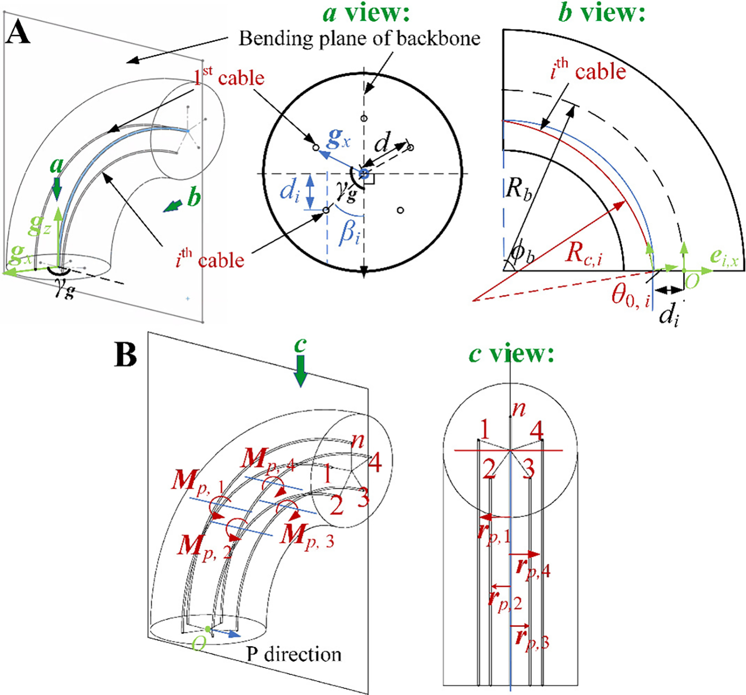
(A). Bending configuration for one section of the arm driven by multiple cables. (B). External moments applied by multiple cables to the soft section in the P direction.

The distance between the incident point of the i^th cable and the neutral plane is calculated as:

$$d_i=d\mathrm{c}\mathrm{o}\mathrm{s}{\beta }_{i}i=1,2,3\dots$$ (19)

In the bending plane of the i^th cable (Fig. 3A), which is parallel to the bending plane of the backbone and contains the i^th cable, the external force condition is analyzed as the single cable-driven case:

$$\left\{\begin{array}{c}{\mathit{F}}_{r,i}=T_i\left[\begin{array}{c}-\mathrm{s}\mathrm{i}\mathrm{n}{\theta }_{0,i}\\ \mathrm{c}\mathrm{o}\mathrm{s}{\theta }_{0,i}\end{array}\right]\\ \left|{\mathit{M}}_{r,i}\right|=\left|-T_i{d}_i\mathrm{c}\mathrm{o}\mathrm{s}{\theta }_{0,i}\right|\\ {\theta }_{0,i}=\alpha -\mathrm{a}\mathrm{r}\mathrm{c}\mathrm{s}\mathrm{i}\mathrm{n}\left(\left(1-{\kappa }_b{d}_i\right)\frac{{\kappa }_{c,i}}{{\kappa }_b}\mathrm{s}\mathrm{i}\mathrm{n}\alpha \right)\\ T_i=\frac{K_c}{{\kappa }_{c,i}}\left\{\left(\frac{1}{{\kappa }_b}-d_i\right)(1-\mathrm{c}\mathrm{o}\mathrm{s}\alpha )-\frac{1}{{\kappa }_{c,i}}\left(1-\mathrm{c}\mathrm{o}\mathrm{s}\left(\alpha -{\theta }_{0,i}\right)\right)\right\}\end{array}\right.$$ (20)

where $T_i,{\theta }_{0,i}$, and ${\kappa }_{c,i}$ are the cable tension, incident angle and curvature of the i^th cable, respectively, and ${\mathit{F}}_{r,i}$ and ${\mathit{M}}_{r,i}$ are the support force and moment components induced by the i^th cable, respectively, in local frame ${\mathit{e}}_i$ (Fig. 3A).

Then, one can calculate the total bending moment applied by the cables for the section:

$$\left|M\right|=\left|\sum _{i=1}^n-M_{r,i}\right|=K_b{\kappa }_b$$ (21)

Furthermore, since there is no bending deformation in the direction perpendicular to the bending direction, and based on assumption (A3), the total external moment applied by cables in the $P$ direction with respect to $O$ (Fig. 3B) is zero:

$$\sum _{i=1}^n{M}_{p,i}=0$$ (22)

where ${\mathit{M}}_{p,i}$ is the external moment applied by the i^th cable with respect to $O$, in the $P$ direction (Fig. 3B).

The arm $r_{p,i}$ of the external forces for ${\mathit{M}}_{p,i}$ is the distance between the bending plane of the i^th cable and the bending plane of the backbone (Fig. 3B), whose direction is perpendicular to the bending plane with the magnitude:

$$r_{p,i}=d\mathrm{s}\mathrm{i}\mathrm{n}{\beta }_i$$ (23)

Thus, the lateral moment ${\mathit{M}}_{p,i}$ applied by the i^th cable is derived as:

$${\mathit{M}}_{p,i}={\mathit{F}}_{T,i,y}\times {\mathit{r}}_{p,i}+{\int }_0^{l_i} {\mathit{\rho }}_{i,y}^e(s)\times {\mathit{r}}_{p,i}ds=-{\mathit{F}}_{r,i,y}\times {\mathit{r}}_{p,i}$$ (24)

where ${\mathit{F}}_{T,i,y},{\mathit{\rho }}_{i,y}^e$, and ${\mathit{F}}_{r,i,y}$ are the components along ${\mathit{e}}_{i,y}$ axis (or ${\mathit{g}}_z$ axis) of the ${\mathit{F}}_{T,i},{\mathit{\rho }}_i^e$, and ${\mathit{F}}_{r,i}$, respectively.

Then, based on equations (19)–(24) and the geometric relationships, the kinematic model for a soft section of the arm actuated by multiple cables is derived as:

$$\left\{\begin{array}{c}\sum _{i=1}^n T_{i}d\mathrm{c}\mathrm{o}\mathrm{s}{\theta }_{0,i}\mathrm{c}\mathrm{o}\mathrm{s}{\beta }_i=K_b{\kappa }_b\\ \sum _{i=1}^n T_{i}d\mathrm{c}\mathrm{o}\mathrm{s}{\theta }_{0,i}\mathrm{s}\mathrm{i}\mathrm{n}{\beta }_i=0\\ {\theta }_{0,i}=\alpha -\mathrm{a}\mathrm{r}\mathrm{c}\mathrm{s}\mathrm{i}\mathrm{n}\left(\left(1-{\kappa }_b{d}_i\right)\frac{{\kappa }_{c,i}}{{\kappa }_b}\mathrm{s}\mathrm{i}\mathrm{n}\alpha \right)\\ T_i=\frac{K_c}{{\kappa }_{c,i}}\left\{\left(\frac{1}{{\kappa }_b}-d_i\right)(1-\mathrm{c}\mathrm{o}\mathrm{s}\alpha )-\frac{1}{{\kappa }_{c,i}}\left(1-\mathrm{c}\mathrm{o}\mathrm{s}\left(\alpha -{\theta }_{0,i}\right)\right)\right\}\\ l_i=R_{c,i}\left({\varphi }_b-2{\theta }_{0,i}\right)=\frac{1}{{\kappa }_{c,i}}\left(L{\kappa }_b-2{\theta }_{0,i}\right)\end{array}\right.$$ (25)

In the forward mapping from actuation to arm configuration, given the cable lengths $l_i$, the backbone curvature ${\kappa }_b$ and the bending orientation ${\gamma }_{\mathit{g}}$ (manifested via ${\beta }_i$ in equation (18)) are obtained by solving the equation (25). ${\theta }_{0,i},{\kappa }_{c,i}$, and $T_i$ are intermediate variables, $d,L,K_c$, and $K_b$ are constants, and ${\varphi }_b,\alpha$ are fully determined by ${\kappa }_b$. Therefore, in the forward mapping problem, there are $(3n+2)$ unknowns and $(3n+2)$ independent equations. In the inverse mapping problem, the lengths $l_i$ for different cables are calculated based on the desired reference values of ${\kappa }_b$ and ${\gamma }_{\mathit{g}}$ by solving the same equation (25). It is noticed that $n$ (the number of the cables) is required to be larger than 2 to achieve a redundant actuation system for all of the bending orientations considering the limitation that $T_i$ is non-negative (in the inverse mapping, considering the equation (25), substituting ${\beta }_i$ by using ${\gamma }_{\mathit{g}}$, the numbers of independent equations and the unknown variables are ($3n+2$) and ($4n$), respectively). The initial guess of the nonlinear system is obtained by solving the last three rows in (25), where we assume that there is no transverse deformation of the cables: ${\theta }_{0,i}=0$.

C. Modeling of a Multi-Section Soft Arm

For the multi-section soft robotic arm, the kinematic model between the task space configuration (in particular, the end position) and the bending configuration for each section is built by using homogeneous transformation matrices [14]. Specifically, considering the thickness of the rigid endcaps, one can divide each section of the arm into three parts: straight, bending, and straight. The transformation matrix $T_{i,e}^{i,s}$, which transforms vectors in the end frame ${\mathrm{\Sigma }}_{i,e}$ to those in the base frame ${\mathrm{\Sigma }}_{i,s}$ for the i^th section (Fig. 4A), is given by:

$$T_{i,e}^{i,s}=\left[\begin{array}{cc}I& {\mathit{p}}_{0,i}\\ 0& 1\end{array}\right]\left[\begin{array}{cc}{R}_z\left({\gamma }_i\right)& 0\\ 0& 1\end{array}\right]\left[\begin{array}{cc}{R}_y\left({\varphi }_{b,i}\right)& {\mathit{p}}_i\\ 0& 1\end{array}\right]\left[\begin{array}{cc}{R}_z\left(-{\gamma }_i\right)& 0\\ 0& 1\end{array}\right]\left[\begin{array}{cc}I& {\mathit{p}}_{0,i}\\ 0& 1\end{array}\right]$$ (26)

where ${\varphi }_{b,i}$ and ${\gamma }_i$ (${\gamma }_i$ is with respect to a general base frame ${\mathrm{\Sigma }}_{i,s}$ that is not dependent on the cable distribution) are the bending angle and orientation for the i^th section, respectively, ${\mathit{p}}_i={\left[\begin{array}{lll}\left(1-\mathrm{c}\mathrm{o}\mathrm{s}{\varphi }_{b,i}\right)/{\kappa }_{b,i}& 0& \mathrm{s}\mathrm{i}\mathrm{n}{\varphi }_{b,i}/{\kappa }_{b,i}\end{array}\right]}^T$ is the in-plane displacement from the base to tip for the i^th section, ${\kappa }_{b,i}$ is the curvature of the backbone of the i^th section, ${\mathit{p}}_{0,i}={\left[\begin{array}{lll}0& 0& h\end{array}\right]}^T$ is the displacement of the straight part and $h$ is the thickness of the endcaps. $I$ is a three-dimensional identity matrix, $R_z\left({\gamma }_i\right),R_y\left({\varphi }_{b,i}\right)$, and $R_z\left(-{\gamma }_i\right)$ are the 3D rotation matrices around the z-axis, y-axis and z-axis for the angle ${\gamma }_i,{\varphi }_{b,i}$, and $-{\gamma }_i$, respectively.

Figure 4. Modeling of a multi-section soft robotic arm.

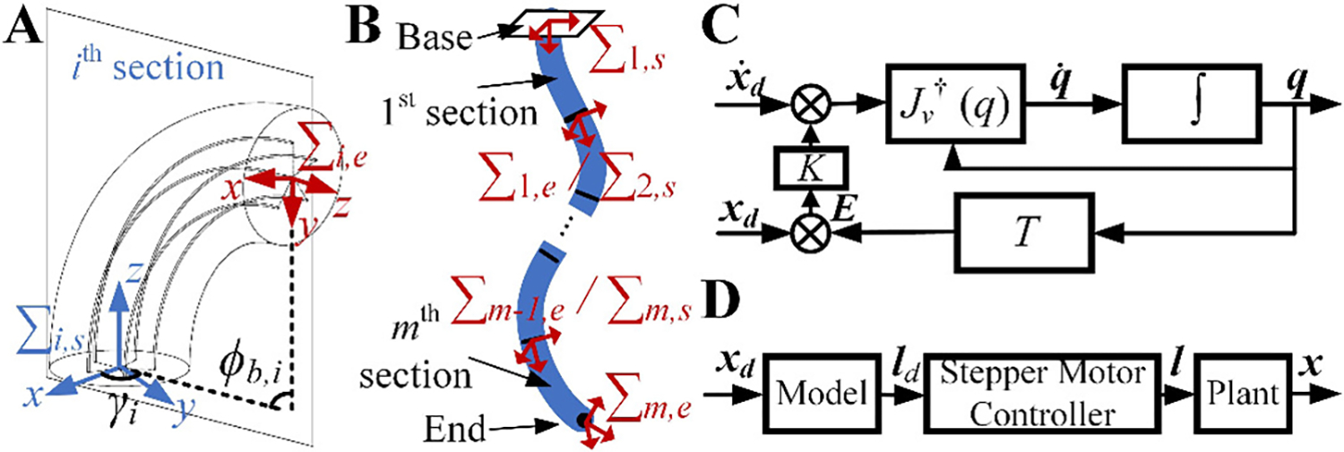
(A). Variables of bending configuration for one section. (B). Local frames for different sections. (C). The inverse kinematics solver for the bending configurations of different sections based on the reference of the end position. (D). Open loop control of the soft robotic arm based on the proposed model. $\mathit{x}$ and $\mathit{l}$ are the end position of the soft robotic arm and the actuation cable lengths, respectively, for which ${\mathit{x}}_d$ and ${\mathit{l}}_d$ are the corresponding target values.

The transformation matrix $T_{m,e}^{1,s}$ which transforms vectors in the end frame ${\mathrm{\Sigma }}_{m,e}$ to those in the base frame ${\mathrm{\Sigma }}_{1,s}$ of the $m$-section arm, and the end position of the arm ${\mathit{p}}_t^{1,s}$ (subscript “t“ for “tip”) in ${\mathrm{\Sigma }}_{1,s}$ (Fig. 4B) can be calculated as:

$$T_{m,e}^{1,s}=\prod _{i=1}^m{T}_{i,e}^{i,s}$$ (27)

$${\mathit{p}}_t^{1,s}=T_{m,e}^{1,s}\cdot {\mathit{p}}_t^{m,e}$$ (28)

where ${\mathit{p}}_t^{m,e}={\left[\begin{array}{llll}0& 0& 0& 1\end{array}\right]}^T$.

For the inverse kinematics [21], the linear velocity Jacobian matrix $J_v$ for the end position of the $m$-section arm with respect to the variables of bending configuration of each section is calculated as:

$$J_v=J_{{\mathit{p}}_t^{1,s}}(\mathit{q})=\left[\begin{array}{lll}\frac{\partial {\mathit{p}}_t^{1,s}}{\partial q_1}& \dots & \frac{\partial {\mathit{p}}_t^{1,s}}{\partial q_{2m}}\end{array}\right]$$ (29)

where $\mathit{q}={\left[\begin{array}{lllll}{\gamma }_1& {\kappa }_{b,1}& \dots & {\gamma }_m& {\kappa }_{b,m}\end{array}\right]}^T$ is the set of variables of the bending configurations of all sections. The calculated $J_v$ is omitted for brevity and a small value ${\delta }_{\kappa }$ is added to ${\kappa }_{b,i}$ when ${\kappa }_{b,i}\to 0$ for numerical stability. At least two sections are required for the arm to provide redundancy for tracking desired end positions in 3D space.

Once $J_v$ is obtained, one can use the following method to approach the configurations given the desired task space output (inverse kinematics) by using the Levenberg–Marquardt method [22]:

$$\dot{\mathit{q}}={J_v}^{†}𝒱+\left(I-{J_v}^{†}{J}_v\right){\dot{\mathit{q}}}_0$$ (30)

Where ${J_v}^{†}={J_v}^T{\left(J_v{J_v}^T+k^{2}I\right)}^{-1}$ is the pseudo inverse of $J_v,I$ is an identity matrix, $k$ is a small positive number, $𝒱={\dot{\mathit{x}}}_d(t)$ is the velocity vector of the tracking trajectory ${\mathit{x}}_d(t)$ (subscript “$d$” for “desired”), ${\dot{\mathit{q}}}_0$ is any vector with the shape of $\dot{\mathit{q}}$ and set to zero for the minimum energy criterium.

By using the Euler method [23] to integrate the velocities, the references for the bending configuration variables are calculated:

$$\mathit{q}\left(t_{k+1}\right)=\mathit{q}\left(t_k\right)+{J_v}^{†}\left(\mathit{q}\left(t_k\right)\right)\cdot {\dot{\mathit{x}}}_d\left(t_k\right)\cdot \mathrm{\Delta }t$$ (31)

where $\mathit{q}\left(t_k\right)$ and $\mathit{q}\left(t_{k+1}\right)$ denote $\mathit{q}$ at the time steps $t_k$ and $t_{k+1}$, respectively.

Closed-loop feedback is further implemented in the solver (Fig. 4C) to reduce the error accumulated by the numerical integration with (31):

$$\dot{\mathit{q}}={J_v}^{†}(\mathit{q})\left({\dot{\mathit{x}}}_d+K\cdot \mathit{E}\right)$$ (32)

where $\mathit{E}={\mathit{x}}_d-T_{m,e}^{1,s}(\mathit{q})\cdot {\mathit{p}}_t^{m,e}$ is the feedback error and $K$ is a positive diagonal gain matrix. Once $\mathit{q}$ is obtained, we can use the equation (25) to calculate the cable lengths $l_i$ for different actuation cables for all sections. Thus, by combining the kinematic model for a multi-section arm and the static model for single section, an analytical model can be built for handling the modeling of a soft arm with an arbitrary number of sections.

IV. Results

A. Baseline Model for the Soft Robotic Arm

Extensive experiments have been conducted to validate the proposed model. For a fair comparison, a static baseline model was built based on the same assumptions (including the PCC assumption), except the consideration of the transverse deformation induced by the cables. The multi-section part of the baseline model was kept the same as that of the proposed model. In this way, the influence of considering the transverse deformation can be isolated from those of other factors. Note that the proposed model reduces to the baseline model once the transverse deformation effect is ignored (assigning ${\theta }_{0,i}=0$). The derived baseline model shares the same form as in the existing literature [14], where the curvature ${\kappa }_{c,i}$ and the length $l_i$ of the i^th cable in a section (blue curve in Fig. 3A) are derived as:

$$\frac{1}{{\kappa }_b}=\frac{1}{{\kappa }_{c,i}}+d_i$$ (33)

$$l_i=R_{c,i}\cdot {\varphi }_b=\frac{{\kappa }_b}{{\kappa }_{c,i}}L$$ (34)

where $d_i$ is derived from equation (19), ${\kappa }_b$ and $L$ are the curvature and the length of the backbone, respectively.

B. Parameter Identification

The geometric parameters including ($L,d$) were measured directly from the prototype. The total length of the two-section arm was 206 mm and the diameter of the soft arm $D$ was 28 mm. The bending stiffness $K_b$ for a single soft section was calculated by using equations (11) and (16) assuming ${\theta }_0\approx 0$ when ${\varphi }_b$ was small, where $T$ and ${\varphi }_b$ were measured by a force sensor and a motion capture system when a single section was driven by one cable, respectively.

The relationship between a single cable contraction length $\mathrm{\Delta }l$ and ${\varphi }_b$ (Fig. 5B) was obtained in experiments for one soft section driven by a single cable, where the experimental results (Fig. 5B) were used to identify $K_c$ by using equation (17). The experimental results and the estimations of the bending deformation of one section driven by one cable based on the baseline model and the proposed model (equation (17)) with the identified parameters are shown in Fig. 5B. The experimental setups for identifying $K_b$ and $K_c$, the measured geometry parameters, and identified parameters $\left(L,d,K_b,K_c\right)$ are elaborated in Supplementary Materials (S3).

Figure 5. Experiment results for a single section of the soft robotic arm.

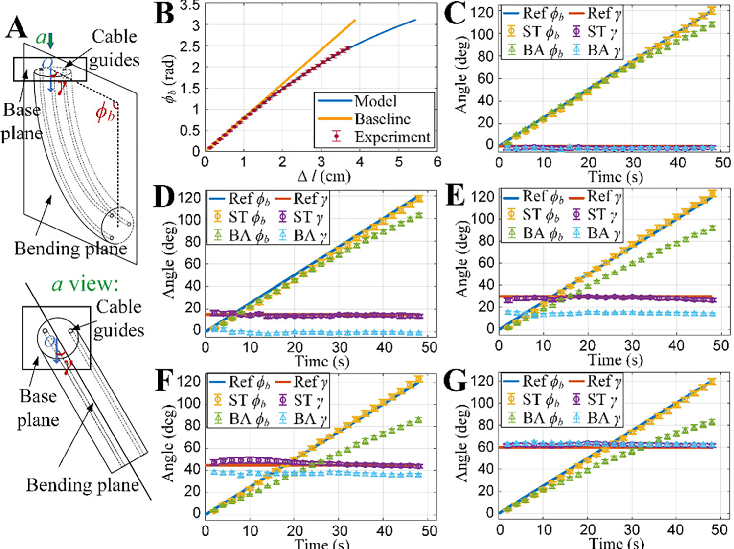
(A). The bending configuration of one section in experiments. (B). The relationship between cable contraction $\mathrm{\Delta }l=L-l$ and bending angle ${\varphi }_b$ with single cable actuation, comparing the predictions of the proposed model and the baseline model with the experimental data. (C). Tracking different bending angle ${\varphi }_b$ when $\gamma =0^{\circ }$ using the baseline model (BA) and the proposed model (ST). (D). Tracking different ${\varphi }_b$ when $\gamma ={15}^{\circ }$. (E). Tracking different ${\varphi }_b$ when $\gamma ={30}^{\circ }$. (F). Tracking different ${\varphi }_b$ when $\gamma ={45}^{\circ }$. (G). Tracking different ${\varphi }_b$ when $\gamma ={60}^{\circ }$. The error bars denote the standard deviations of three runs for each bending configuration in the results.

C. Experimental Results for a Single Section

The single cable actuation results (Fig. 5B) showed that, compared with the baseline model, the proposed static model was better in describing the nonlinear relationship between the cable actuation and the bending angle for the soft robotic arm, especially when the bending angle was relatively large. The simulation results of the proposed model and the real experiment data showed good agreements (Fig. 5B), validating the prediction accuracy of the model. The results also indicated that the proposed model maintained high accuracy when the transverse deformation induced by the cable became more significant. The prediction by the baseline model, on the other hand, became worse when such effects became non-negligible under stronger actuation. After the model parameters were identified, extensive experiments were conducted to compare the accuracy of the baseline model and the proposed model (equation (25)), where an open loop control without feedback was used (Fig. 4D). A single section of the arm was used to track different bending angles ${\varphi }_b$ in specific bending orientations $\gamma$ by using different models (Fig. 5A). The experimental setups, strategy for multi-cable redundancy, data processing methods for the results, and the high computation efficiency of the models (taking less than 1 ms to solve in Matlab) are elaborated in Supplementary Materials (S3).

The experiment results of the bending configurations (${\varphi }_b,\gamma$) of the single section arm controlled by multiple cables by using different models are shown in Fig. 5C–G. In the experiments, it was shown that the tracking accuracy of the proposed static model was significantly better than the baseline model in the experimental range (Fig. 5C–G), indicating the importance and effectiveness of considering the transverse deformation of the cable in the proposed robotic arm. In particular, the tracking errors in ${\varphi }_b$ and $\gamma$ for the proposed model were small for different bending configurations. In comparison, the tracking error in ${\varphi }_b$ for the baseline model increased together with the target ${\varphi }_b$ when the target $\gamma$ was fixed, while the tracking error in $\gamma$ for the baseline model was almost constant and was considerable in some cases despite the changing of the target ${\varphi }_b$ when the target $\gamma$ was fixed.

Moreover, it was also shown that in the experiment range, the tracking error in ${\varphi }_b$ for the baseline model increased with larger target $\gamma$ when the target ${\varphi }_b$ was fixed. The maximum ${\varphi }_b$ tracking error increased from about 12 degrees to about 37 degrees when the target $\gamma$ increased from 0 to 60 degrees, respectively. The $\gamma$ tracking error for the baseline model increased from about 0 to about 16 degrees when the target $\gamma$ increased from 0 to 30 degrees, respectively, and then decreased to near 0 when the target $\gamma$ increased to 60 degrees. It was noticed that for both models, the $\gamma$ tracking error approached 0 when target $\gamma$ was 0 and 60 degrees, which was attributed to a single effective cable contraction and two effective cable contractions with the same contraction length, respectively. Specifically, when the target $\gamma$ was 0, there was only one effective actuation cable (the other two cable were almost slack) for both the baseline model and the proposed model, and the bending orientation $\gamma$ in the experiment naturally stayed around 0, which was the same as the orientation of the actuation cable. When the target $\gamma$ was 60 degrees, the two actuation cables shared the same contraction length (the third cable was almost slack) for both the baseline model and proposed model, and $\gamma$ in the experiment stayed near 60 degrees because of the actuation and structure symmetry.

A trajectory tracking experiment for the end of the single section was further conducted where the trajectory reference was included in its workspace. The experiment showed that the average tracking error of the single section (1.58 cm) by using the proposed model (equation (25)) was about 35% smaller than that (2.43 cm) of the baseline model (Fig. 6A) validating the effectiveness of the proposed model, and the soft section had flexible and versatile bending configurations (Fig. 6B–C). A video of these experiments and those in Section IV–D can be viewed at https://youtu.be/I-e1PxHwG1Y (Supplementary Video).

Figure 6. Experiment results for a single section of the soft robotic arm tracking a circular trajectory.

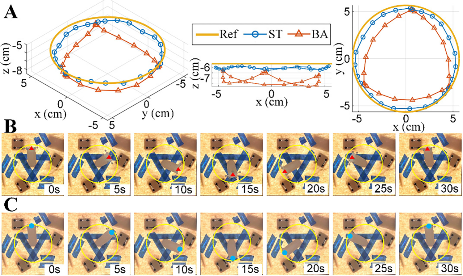
(A). Trajectories of the end position of the single section by using the baseline model (BA) and the proposed model (ST). (B). Illustration of movement and bending of the single section by using BA. (C). Illustration of movement and bending of the single section by using ST. In (B) and (C), yellow curves indicate the reference trajectory and red/blue dots indicate the tip of the arm.

D. Experimental Results for a Two-Section Soft Robotic Arm

A multi-section arm was assembled and utilized for the comparison of the baseline model and the proposed model, and its performance was further evaluated. For simplicity, a two-section arm was assembled and controlled to track a circular trajectory within its workspace by using the baseline model and the proposed model. The experiment results showed that, the average tracking error with the proposed model (3.76 cm) was about 36% smaller compared with the baseline model (5.92 cm), and the trajectory achieved with the open loop controller based on the proposed model was closer to the reference (Fig. 7A–C; also see the Supplementary Video). The tracking error of the two-section soft arm was larger compared with that with a single section, which might be attributed to the error accumulation between multiple sections and a more prominent gravity influence for the base section of the arm.

Figure 7. Experiment results for a two-section soft robotic arm.

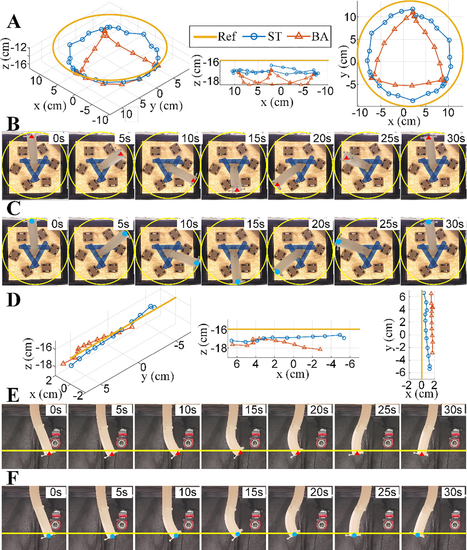
(A). Trajectories of the end position of the arm tracking a circular path by using the baseline model (BA) and the proposed static model (ST). (B). Illustration of movement and bending of the arm tracking a circular path by using BA. (C). Illustration of movement and bending of the arm tracking a circular path by using ST. (D). Trajectories of the end position of the arm tracking a straight path by using BA and ST. (E). Illustration of movement and bending of the arm tracking a straight path by using BA. (F). Illustration of movement and bending of the arm tracking a straight path by using ST. In (B), (C), (E), and (F), yellow curves indicate the reference trajectory and red/blue dots indicate the tip of the arm.

In addition, the two-section arm was controlled to track a straight trajectory within its workspace by using the models, where the average tracking error (1.70 cm) of the proposed model was about 52% smaller than that of the baseline model (3.52 cm) (Fig. 7D–F) showing the advantage of the proposed model. Besides the comparison between the proposed model and the baseline model, by evaluating a normalize tracking error (the ratio of the static tracking error in open-loop control over the total arm length), it was found that the tracking error based on the proposed model (about 18.3%, 8.3% in circular, straight tests, respectively) was comparable to that based on a state-of-art FEM modeling approach (about 12.5%) in [17], while the proposed model was much more computationally efficient (see S3 in Supplementary Material).

In summary, the extensive experiments showed the advantage of the proposed static model as compared to a baseline model and validated the flexibility and dexterity of the proposed soft robotic arm.

V. Discussion and Conclusion

In this work, we designed an octopus-inspired soft robotic arm and developed a novel kinematic model to characterize its flexible movements. The modular design of the soft arm enabled longer arm prototypes and permitted a decoupling cable actuation system for different sections that simplified the modeling. The hybrid fabrication method of 3D printing and casting resulted in low-cost and easy-to-build prototypes. An analytical static model was built to capture the transverse deformation of the cable during actuation, which was largely ignored in the literature.

Extensive experiments were conducted to validate the proposed model and the static baseline model was used for a fair comparison. The modeling accuracy was evaluated in the cable actuation experiments (Fig. 5B) and tracking experiments (Fig. 5–7). The results of tracking experiments for a single section of the soft arm showed an evident advantage and smaller tracking errors for the proposed model over the baseline model in terms of bending angle, orientation, and the end position of the arm. Experiments with a two-section arm further supported the efficiency of the proposed model in tracking circular and straight trajectories for the endpoint and demonstrated the dexterity of the proposed soft arm.

We note that our modeling approach was not only motivated by and particularly relevant to the proposed modular cable-driven soft robotic arm, but also applicable to many other cable-driven robotic arms, especially those not using rigid spacers, examples of which are abundant [24], [25]. Even for the soft arms with multiple rigid spacers, the transverse deformation phenomenon would still exist in the areas where the cables and the soft body interact directly.

For future work, first, we plan to relax the current geometric assumption (PCC assumption) for the soft arm by considering the moments generated by the gravity and external forces, using an iterative approach similar to that in Fairchild et al [26]. We will also explore the related dynamic model with external interactions. Finally, we will develop integrated embedded sensors (e.g., soft strain sensors) for the soft robotic arm, so that real-time bending configuration data for the arm are made available for feedback control.

REFERENCES

- [1].Xie Z, Domel AG, An N, et al. , “Octopus arm-inspired tapered soft actuators with suckers for improved grasping,” Soft robotics, vol. 7, no. 5, pp. 639–648, 2020. [DOI] [PubMed] [Google Scholar]
- [2].Palmieri P, Melchiorre M, and Mauro S, “Design of a lightweight and deployable soft robotic arm,” Robotics, vol. 11, no. 5, p. 88, 2022. [Google Scholar]
- [3].Liang X, Cheong H, Sun Y, Guo J, Chui CK, and Yeow C-H, “Design, characterization, and implementation of a two-dof fabric-based soft robotic arm,” IEEE Robotics and Automation Letters, vol. 3, no. 3, pp. 2702–2709, 2018. [Google Scholar]
- [4].Wang X, Kang H, Zhou H, Au W, Wang MY, and Chen C, “Development and evaluation of a robust soft robotic gripper for apple harvesting,” Computers and Electronics in Agriculture, vol. 204, p. 107552, 2023. [Google Scholar]
- [5].Cianchetti M, Ranzani T, Gerboni G, De Falco I, Laschi C, and Menciassi A, “Stiff-flop surgical manipulator: Mechanical design and experimental characterization of the single module,” in 2013 IEEE/RSJ international conference on intelligent robots and systems, pp. 3576–3581, IEEE, 2013. [Google Scholar]
- [6].Diodato A, Brancadoro M, De Rossi G, et al. , “Soft robotic manipulator for improving dexterity in minimally invasive surgery,” Surgical innovation, vol. 25, no. 1, pp. 69–76, 2018. [DOI] [PubMed] [Google Scholar]
- [7].Wang Z, Hirai S, and Kawamura S, “Challenges and opportunities in robotic food handling: A review,” Frontiers in Robotics and AI, vol. 8, p. 789107, 2022. [DOI] [PMC free article] [PubMed] [Google Scholar]
- [8].Chen X, Zhang X, Huang Y, Cao L, and Liu J, “A review of soft manipulator research, applications, and opportunities,” Journal of Field Robotics, vol. 39, no. 3, pp. 281–311, 2022. [Google Scholar]
- [9].Katzschmann RK, Della Santina C, Toshimitsu Y, Bicchi A, and Rus D, “Dynamic motion control of multi-segment soft robots using piecewise constant curvature matched with an augmented rigid body model,” in 2019 2nd IEEE International Conference on Soft Robotics (RoboSoft), pp. 454–461, IEEE, 2019. [Google Scholar]
- [10].Xing Z, Zhang J, McCoul D, Cui Y, Sun L, and Zhao J, “A super-lightweight and soft manipulator driven by dielectric elastomers,” Soft robotics, vol. 7, no. 4, pp. 512–520, 2020. [DOI] [PubMed] [Google Scholar]
- [11].Li C and Rahn CD, “Design of continuous backbone, cable-driven robots,” J. Mech. Des, vol. 124, no. 2, pp. 265–271, 2002. [Google Scholar]
- [12].Lai J, Huang K, Lu B, Zhao Q, and Chu HK, “Verticalized-tip trajectory tracking of a 3d-printable soft continuum robot: Enabling surgical blood suction automation,” IEEE/ASME Transactions on Mechatronics, vol. 27, no. 3, pp. 1545–1556, 2021. [Google Scholar]
- [13].Mustaza SM, Elsayed Y, Lekakou C, Saaj C, and Fras J, “Dynamic modeling of fiber-reinforced soft manipulator: A visco-hyperelastic material-based continuum mechanics approach,” Soft robotics, vol. 6, no. 3, pp. 305–317, 2019. [DOI] [PubMed] [Google Scholar]
- [14].Webster III RJ and Jones BA, “Design and kinematic modeling of constant curvature continuum robots: A review,” The International Journal of Robotics Research, vol. 29, no. 13, pp. 1661–1683, 2010. [Google Scholar]
- [15].Camarillo DB, Milne CF, Carlson CR, Zinn MR, and Salisbury JK, “Mechanics modeling of tendon-driven continuum manipulators,” IEEE transactions on robotics, vol. 24, no. 6, pp. 1262–1273, 2008. [Google Scholar]
- [16].Renda F, Giorelli M, Calisti M, Cianchetti M, and Laschi C, “Dynamic model of a multibending soft robot arm driven by cables,” IEEE Transactions on Robotics, vol. 30, no. 5, pp. 1109–1122, 2014. [Google Scholar]
- [17].Morales Bieze T, Kruszewski A, Carrez B, and Duriez C, “Design, implementation, and control of a deformable manipulator robot based on a compliant spine,” The International Journal of Robotics Research, vol. 39, no. 14, pp. 1604–1619, 2020. [Google Scholar]
- [18].Trivedi D, Lotfi A, and Rahn CD, “Geometrically exact models for soft robotic manipulators,” IEEE Transactions on Robotics, vol. 24, no. 4, pp. 773–780, 2008. [Google Scholar]
- [19].Renda F, Armanini C, Mathew A, and Boyer F, “Geometrically-exact inverse kinematic control of soft manipulators with general threadlike actuators’ routing,” IEEE Robotics and Automation Letters, vol. 7, no. 3, pp. 7311–7318, 2022. [Google Scholar]
- [20].Wu Y, Yim JK, Liang J, Shao Z, Qi M, Zhong J, Luo Z, Yan X, Zhang M, Wang X, et al. , “Insect-scale fast moving and ultrarobust soft robot,” Science robotics, vol. 4, no. 32, p. eaax1594, 2019. [DOI] [PubMed] [Google Scholar]
- [21].Sciavicco L and Siciliano B, Modelling and control of robot manipulators. Springer Science & Business Media, 2001. [Google Scholar]
- [22].Weisstein EW, “Levenberg-marquardt method,” https://mathworld.wolfram.com/, 2000.
- [23].Epperson JF, An introduction to numerical methods and analysis. John Wiley & Sons, 2021. [Google Scholar]
- [24].Wang H, Chen W, Yu X, Deng T, Wang X, and Pfeifer R, “Visual servo control of cable-driven soft robotic manipulator,” in 2013 IEEE/RSJ International Conference on Intelligent Robots and Systems, pp. 57–62, IEEE, 2013. [Google Scholar]
- [25].Deng T, Wang H, Chen W, Wang X, and Pfeifer R, “Development of a new cable-driven soft robot for cardiac ablation,” in 2013 IEEE International Conference on Robotics and Biomimetics (ROBIO), pp. 728–733, IEEE, 2013. [Google Scholar]
- [26].Fairchild P, Shepard N, Mei Y, and Tan X, “Semi-physical modeling of soft pneumatic actuators with stiffness tuning,” ASME Letters in Dynamic Systems and Control, pp. 1–6, 2023. [Google Scholar]
Associated Data
This section collects any data citations, data availability statements, or supplementary materials included in this article.