

Abstract
This study examines long-term air temperature trends in Bhubaneswar, a rapidly urbanizing coastal city in eastern India, using data from 1901 to 2023. By analyzing maximum, minimum, and mean temperatures, we assess both natural climate variability and anthropogenic influences, including urban expansion. Statistical techniques such as homogenization, persistence analysis, and low-pass filtering reveal a pronounced warming trend, particularly in minimum temperatures, as an indication of an intensifying urban heat island effect. A weak but positive correlation between minimum temperature and population growth supports the role of urbanization in shaping local climate. These findings contribute to understanding urban climate evolution in tropical coastal settings where natural and human factors interact. Our results underscore minimum temperatures compared to maximum temperatures, indicating a warming trend likely driven by anthropogenic activities. Regression analysis between population growth and minimum temperature affirms a weak but notable positive correlation, indicating the gradual intensification of Bhubaneswar’s local microclimate due to urban development. This study contributes to understanding climate dynamics in tropical, coastal, and urban regions, where natural and human factors converge, shaping distinct local climate patterns. Nonetheless, the climatic trends are less pronounced than the interannual fluctuations in temperature measurements. The little climatic differences across several generations are unlikely to have influenced human activities compared to the substantial impacts of interannual temperature variability.
Keywords: Mean temperature, Homogenization, Anthropogenic, Heat island, Coastal odisha
Subject terms: Climate sciences, Atmospheric science, Climate change
Introduction
The study of climate change has gained increasing attention over the past few decades, particularly in relation to modelling long-term climate trends and evaluating the role of human activities in influencing these changes. Analyzing extended meteorological time series is central to these efforts. Among climatic variables, temperature is considered a primary indicator of climate variability, reflecting changes in the kinetic energy of atmospheric gases.
Urban environments exhibit distinct temperature patterns, often influenced by anthropogenic factors such as greenhouse gas emissions, land-use changes, and infrastructure growth. The urban heat island (UHI) effect is characterized by elevated temperatures in urban areas relative to surrounding rural regions, which has been extensively documented1–7. This effect is closely linked to city size, density, and expansion rate.
Bhubaneswar, the capital of Odisha on India’s east coast, has a complicated urban environment that has perplexed urban climatologists. The temperate city was a favoured location for residents to create their homes in the 1970 s, 1980 s, and, to a lesser degree, in the early 1990s. Nonetheless, it has become exceedingly uncomfortable in the twenty-first century, especially among the vulnerable population. Three factors influence its operation across several spatial–temporal scales: terrain, urban form, and proximity to the sea. In the last 23 years, the population has also approximately doubled due to the city’s expansion in business establishments, small-scale industries, and real estate businesses with high-rise apartments. Along the eastern Ghat Mountains’ axis, the city of Bhubaneswar sits on the eastern coastal plains. The city is located southwest of the Mahanadi River and has an average elevation of 45 m above sea level. Bhubaneswar’s soil types are composed of 10% sandstone, 25% alluvial and 65% laterite. The city has a slight dumbbell form, with most of its growth occurring in the north, northeast and southwest.
According to the Köppen Climate Classification, Bhubaneswar has a tropical savanna climate with hot, dry summers and wet, mild winters. The temperature varies from 8 to 46 degrees Celsius. The average daily minimum temperature during winter (December to February) is 16.5 degrees Celsius, and the daily minimum temperature drops below 10 degrees Celsius on some days in January, February, November, and December. In summer, the average daily maximum temperature during pre-monsoon months (March to May) is 36.5 degrees Celsius. However, the daily maximum temperature rises above 45 degrees Celsius on some days in April, May, and June, and the highest maximum temperature of 46.9 degrees Celsius was recorded on 5th June 2012. Most rainfall occurs from June to September in the south-west monsoon season, and the annual total rainfall is 1638 mm based on the 1981–2010 climatological table of IMD. When western disturbances travel far north of the city in winter, Odisha experiences warm and chilly daytime temperatures. During the pre-monsoon season (March to May), severe thunderstorms occur on some days, causing lightning, hailstorms, and precipitation. The pre-monsoon month’s high insolation catalyses the circulation of sea breezes. The winds blow mainly along the southwest/northeast axis during pre-monsoon and southwest monsoon.
The study aimed to determine whether the climate features varied at Bhubaneswar. So, monthly mean data of maximum ( ), Minimum (
 ), and air temperature (
 ) from 1901 to 2023 are obtained from different sources. The air temperature here refers to the mean temperature of the month, season, or annual averages, and the mean temperature is characterized as the average temperature over a specific period, such as monthly, seasonal or annual averages. RH tests of homogenization were applied to remove discontinuities in the temperature data in the time series. As these yearly-homogenized data are being used for statistical analysis, the normality test of Kolmogorov–Smirnov was also applied and satisfied. In order to (i) recreate the history of this meteorological parameter by finding patterns and comparing them with those of other cities in Asia and Europe, and (ii) assess the impact of the city’s growth on temperature trends, the annual mean temperature data for Bhubaneswar are analyzed. Temperatures are graphed against the years to identify distinct characteristics, like the coldest and warmest years of the century. The trend analysis was conducted via low-pass numerical filters. A notable aspect of urbanization is the urban heat island (UHI); temperature analysis serves as the method to illustrate the urban heat island effect1,2,4,5,8, and the utilisation of straightforward correlation models offers an adequate elucidation of the minimum temperature trend. Research has been conducted on time series data for persistent analysis to comprehend the association between historical and present data.
The city is infrequently affected by tropical cyclones in pre-monsoon (March to May) and post-monsoon seasons (October to November). Maximum devastation with human casualties occurred during the 1999 super cyclone in October, and also by the FANI Cyclone in 2019 during May. In addition to these calamities, a heat wave is a recurring phenomenon during the pre-monsoon season, and it caused a death toll of around 2042 during the pre-monsoon season in 19989,10. However, Bhubaneswar is vulnerable to natural calamities, and their frequency and intensity have increased in the last 2 to 3 decades, causing acute variability in climatic features. Climatic variability refers to fluctuations in climate conditions, including temperature, over short-term (seasonal) and long-term (inter-annual or decadal) periods.
Data used
Considering the enormous growth of population in the last 3 decades and infrastructural development in Bhubaneswar city, the urban city climate is experienced in and around the observatory site inside the civil aerodrome campus. Multi-storied structures are constructed in the northeastern sector of the observatory, and the location of the observatory is adjacent to city areas. The station’s altitude is 46 m above mean sea level, and its geographical coordinates are Latitude 20°15’N and Longitude 85°50’E. The observatory was established on 1st July 1948. Bhubaneswar station is under WMO, and its code is 42,971. It is a Class-I standard observatory with installed standardized IMD (India Meteorological Department) equipment. Due to the frequent occurrence of meteorological hazards in Odisha state, including Bhubaneswar, the research on climate and its variations is more prevalent in this region for building models in connection with climate change forecasts and modifications introduced by human activities. Though the observatory was established in 1948, daily or mean meteorological parameters have been available since 1952 for Bhubaneswar. The location of Bhubaneswar station in coastal Odisha, along with other surface meteorological observatories in the same climatic region, is shown in Fig. 1 and is generated using ArcGIS Pro Software. [Available at: https://www.esri.com/en-us/arcgis/products/arcgis-pro/trial]. The Base map is prepared using the Ocean map available in the Base map section in the ArcGIS Pro software. Then, the Odisha state shape file and the place shape file are inserted, and the map is prepared.
Fig. 1.
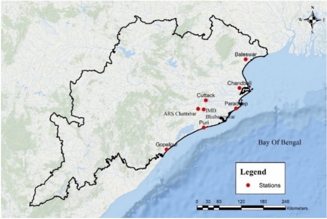
Location of IMD Bhubaneswar and other surface Meteorological Stations over Coastal Odisha [ArcGIS Pro Software.
Available at: https://www.esri.com/en-us/arcgis/products/arcgis-pro/trial].
The Odisha state shape file is downloaded from the Survey of India, Open source online series map section. The data used in this study are obtained from the National Data Centre, IMD, Pune, Office of Special Relief Commissioner, Government of Odisha, and some days from open source website www.ogimet.com.
Most of the dataset contained missing values, particularly in earlier years. To enhance transparency, Table 1 summarizes the quantity of missing data and the strategies used to address these gaps.
Table 1.
Missing data and the strategies used to fill-up missing data.
| Parameter | Years with missing data | Filling method |
|---|---|---|
| TMax | 1901–1951 | Multiple regression using nearby stations (Chandbali & Cuttack) |
| TMin | 1901–1951 | Multiple regression using nearby stations (Chandbali & Cuttack) |
| TMean | 1901–1951 | Averaged Tmax and Tmin |
| Monthly Mean Data (if any) | 1952–1968 | Multiple regression using nearby stations (Chandbali & Cuttack) |
| Daily Data | 1969–2023 | Multiple regression using nearby stations (Chandbali & Cuttack) |
There were data gaps as mentioned in Table 1. Missing daily data were filled up by the multi-regression method using nearby available IMD run stations named Chandbali, and Cuttack by the regression equation as given below:
 |
1 |
where  is intercept,
  &
& are slopes of the line to the best fit, and
  is the random error because the points do not fall on the line. The locations of these six stations are shown in Fig. 1. A similar procedure is followed for missing mean data between 1952 and 1968. The monthly mean maximum and minimum temperatures from 1901 to 1951 are calculated using a regression technique based on Chandbali and Cuttack station data. Initially, missing mean data of Chandbali from 1901 to 1929 were generated by a similar multi-regression technique. There is no significant difference in standard deviation between available data from 1952 to 2023(SD = 3.12 for maximum and 4.03 for minimum) and complete data, including calculated from 1901 to 2023(SD = 3.28 for maximum and 4.03 for minimum). Daily mean temperature data are generated by a daily average of maximum and minimum temperatures from 1969 to 2023. On the other hand, the monthly mean maximum and minimum temperatures from 1901 to 1968 are averaged to determine the monthly mean temperatures. In comparison, daily measurements from 1969 to 2023 were used to produce monthly mean minimum and maximum temperatures. Finally, the annual mean temperature of maximum, minimum, and mean from 1901 to 2023 is used in this research paper.
Methodology
This study utilized long-term meteorological data for Bhubaneswar, Odisha, from 1901 to 2023. The primary sources of data included:
The National Data Centre (NDC), India Meteorological Department (IMD), Pune
The office of the Special Relief Commissioner, Government of Odisha
Open-source meteorological datasets from ww.ogimet.com
The data consisted of monthly and annual mean values of maximum, minimum, and mean air temperatures. Observations were recorded at the IMD Class-I observatory in Bhubaneswar, located 20o15’N latitude and 85o50’E longitude, 46 m above sea level.
These data are not free from artificial discontinuities and artificial discontinuities brought on by non-meteorological causes, which may produce erroneous results by hidden climate change or variability parameters11–15. Therefore, we cannot use it directly for further analysis of persistence, low-pass filter, and comparison of minimum temperature concerning increasing population. The non-meteorological factors are instrumentation, growing trees near the observatory site, change of new observers, shifting of station location, the procedure of calculating the mean temperature and change in a surrounding environment like urbanization or instrument shelter16–18. A time series data’s climate variability or trend should be affected only by weather and climate, called a homogeneous series19. Before attempting other methods, the normality test was conducted on the time series data using a non-parametric Kolmogorov–Smirnov test20–24.
Homogenization process
There are two methods to test the homogeneity of a time series of data: absolute and relative homogeneity techniques. When an attempt is made to make absolute homogeneity testing using single station data, the change or shift detected (or no change) may be caused by the fundamental changes in climate. Therefore, it is preferred to use the relative homogeneity technique in which the homogeneity of the target time series (the station time series to be homogenized) can be tested by comparing it to a reference series, which will be generated using time series data of more than two stations. In this study, a composite reference series is created using six neighbouring stations, such as Balasore, Chandbali, Cuttack, Gopalpur, Paradeep, and Puri, to assess the homogeneity of the target series of Bhubaneswar by using a standard software named RH tests V4. Initially, the composite reference series was tested for homogeneity. Then, the homogenised composite series will be used for further testing of the homogeneity of the target time series data. The time series data (mean air temperature, mean minimum temperature and mean maximum temperature) from 1901 to 2023 of Bhubaneswar will be tested for homogeneity by relative homogeneity testing using composite reference series. The graphical user interface (GUI) is intuitive, and a corresponding reference series is necessary to execute the package within the R environment. The time series data has several breakpoints, and this software can identify these. The penalized maximal T-test (PMT)25 and penalized maximum F-test (PMF)26,27 (a)) can be used to adjust numerous breakpoints. This software incorporates a recursive testing algorithm for time series lag-1 autocorrelation, facilitating the assessment of homogeneity in time series data, with or without a reference series. The issues of uneven false alarm rates and detection power can be mitigated through an empirical penalty function27. Several researchers have used this program to homogenize surface temperature, precipitation, and humidity time series data28–33.
Trends of mean temperature
Homogenized monthly mean temperatures of maximum, minimum and air temperature are used to calculate the annual mean temperature for these parameters. Standard data is generated by taking 30 years of average data of individual parameters. This study considers an average of 30 years (Normal value of Maximum (TMax), Minimum (TMin) and Mean (TMean) temperature) from 1961 to 1990 of respective parameters from the whole time series data from 1901 to 2023. The plotting of the mean annual minimum ( ), maximum (
 ), and air temperature (
 ), along with respective average (Normal) values, is created in Fig. 2. The deviation from the normal will be analysed in Sect."Results & Discussions".
Fig. 2.

Annual Mean Values of Air-Temperature in Bhubaneswar (Odisha, India).
The frequency distribution of mean temperature of  ,
, , and TMean(Grey colour) into 0.5 °C bins over the period 1901–2023 (123 years) are represented in separate histograms as shown in Fig. 3.
Fig. 3.

Distribution Histogram of Air Temperature average maximum (TMax), average minimum (TMin), and average temperature (TMean).
Persistence analysis
Persistence in temperature time series was evaluated using serial correlation techniques:
The one-lag serial correlation coefficient (r1) was computed to assess the degree of autocorrelation.
The test statistics (r1)t was derived using the standard normal distribution at a 95% significance level34
Two-lag and three-lag correlations were examined to confirm the presence of long-term persistence
We aim to study the change in temperature, either an increase, a decrease or no change, by the persistence method in the case of annual and seasonal values.
Different methods are used to search for randomness in the time series data as the common characteristic of low-frequency variation exists, so an attempt has been made to analyse 123 years of mean temperature data for studying persistence in the data to verify the association between current values in a time series and past values35. If persistence exists in the time series of temperature data, the deviation from the mean may last for extended periods. The method introduces a positive serial correlation of slight lags. One-lag serial correlation  is defined as follows to assess the time series’ randomness:
 |
2 |
where  the seasonal or yearly mean air temperature is for the ith year,
  is the variance of the means,
  is the N-year mean of
  and N denotes the length of the series. The one-tail 95% significance point of the Gaussian distribution is used to test for the significance of
  and the test value
  is calculated from
 |
3 |
where  is the Gaussian distribution’s standard normal variate that corresponds to the intended significance level34. For persistence, the first non-random variable must be taken into account. The property
  must be met in order to determine the persistence of the 1st-order linear Markov process36. Two-lag
  and three-lag
  ) serial correlations were calculated from
  and
and  , respectively. If 2
 and
and  are met then persistence might happen.
Trend analysis using low-pass filters
To identify long-term temperature trends, a numerical low-pass filter was employed:
The Ormsby filter was used to smooth high-frequency variations while preserving long-term signals (Mitchell, J.M.,1953; Karl, T.R., & Williams Jr, C.N.,1987).
The cut-off frequencies were set at fr = 1/20 cycles per year and fc = 1/100 cycles per year, removing fluctuations with periods less than 20 years.
The filter length M = 22 was determined based on the Nyquist frequency criterion to maximize filtering accuracy.
The air temperature in Bhubaneswar was described in depth using a numerical low-pass filtering technique to comprehend large-scale dynamics. Each point in the time sequence is created using the weighted mean of the M samples before and after, according to this technique’s characteristics. The filter length determined by the physical criterion is denoted by the integer M. If N is the length of the data set (for this study, N is the number of samples of the annual average temperature), the trend may be found using the expression,
 |
4 |
where t = 1, 2…., N
In the current analysis, the filter  used is an Ormsby filter37, which is defined by.
 )](5).
Here,  and
and  are calculated using
  known as roll-off and cut-off frequencies, respectively. Here, we take into account
  Due to this unit gain and zero phase shift, a low-pass filter does not change the amplitude of the signal in the passing band or cause any shifting in the different harmonics. Considering these qualities, the implementation of a low-pass filter is advantageous. The properties of the filter may be depicted by a frequency response curve seen in Fig. 4.
Fig. 4.

The Low Pass Filter’s Frequency Response in the processing of temperature data.
The following formula can be used to select M in order to obtain high-filtering accuracy ( :
:
 |
6 |
M≈22 is considered in this instance in relation to removing fluctuations in fewer than 20 years. The values.  and
and  cycles per annual were chosen. The formula
  connects the sampling rate to the Nyquist frequency or
Urban heat island
Urbanization-induced temperature rise was assessed by analysing Tmin trends and correlating them with population growth (Oke, T.R., 1974; Landsberg, H.E., 1981). Two statistical models were applied:
 where P is the population.
2. Power-Law Model:  , representing a non-linear relationship.
3. The annual population data from 1950 to 2023 were obtained from worldpopulationreview.com.
4. Regression coefficients and correlation strength (R-values) were computed to quantify the relationship.
Human activities have caused a rise in city temperature, which is also envisaged by the variation between the maximum and minimum temperature trends due to the city’s expansion. The urban heat island effect is more prominent at night, as it is more prevalent in minimum temperatures2,4. Long-term data from neighbouring rural areas is unavailable to support the investigation of the impact of the heat islands on Bhubaneswar. One month of data is available from the newly created Agricultural Research Station in Chattabar, located around 16.7 km west of IMD Bhubaneswar. The station’s geographical coordinates are Latitude 20°15’N, Longitude 85°40’E, at a height of approximately 48 m above mean sea level. The station’s position is depicted in Fig. 1, and the data analysis is presented in Sect."Results & Discussions". As a result of the city’s population increase, its expansion has progressed correspondingly. The disparity between urban and rural temperatures, TU − TR, was analysed, revealing an impact on both minimum and maximum temperatures, with a more prominent influence on minimum temperatures. The rise in the minimum urban temperature correlates with urban expansion and population density. In the case of Bhubaneswar, correlation analysis is conducted by examining the population data from 1950 to 2023 alongside the matching minimum temperatures. The population of Bhubaneswar is sourced from the website https://worldpopulationreview.com/cities/india/bhubaneswar. The subsequent formulations derived from the literature were employed to do regression1,2:
 |
7 |
 |
8 |
The statistical significance of trend estimates was determined using confidence intervals. Results were cross-validated with regional climate studies to ensure consistency38,39. The urban heat island effect was confirmed by comparing the temperature trends of Bhubaneswar with available rural station data (ARS Chattabar, 16, 7 km west of IMD Bhubaneswar). This methodological approach ensures a robust, reproducible framework for analysing century-scale climate variations in Bhubaneswar while accounting for observational biases and external influences.
Results & discussions
Statistical data analysis
The annual average temperature is shown in Fig. 2, indicating the trends of mean temperature values of maximum ( ), minimum (
 ) and air temperature (
 ) from1901 to 2023 in Bhubaneswar. The mean monthly temperature generated from mean daily maximum and minimum temperatures from 1969 to 2023 and the monthly mean values from 1901 to 1968 are used to calculate the mean annual temperature (
 . Over the whole dataset, the mean temperature (TMean) is 270C. From 1901 to 1934, the annual means were generally under this mean value, though a few peaks were there at isolated places. Subsequently, the temperature oscillates approximately around the mean until 1973. Furthermore, the trend exhibits ascending or descending fluctuations over several years relative to the average until 1995. Subsequently, temperatures rose from 1996, consistently above the mean value, with the most significant deviations occurring in 2023 (+ 1.20 °C) and 2009 (+ 1.20 °C). The mean temperature and the mean maximum temperature analysis exhibit a comparable trend. As seen in Fig. 2, the mean value of TMax varied from 1956 to 1990. However, it rose from 1995 relative to the mean maximum temperature for the standard period of 1961 to 1990 and continues to rise. The average temperature over the whole recorded period is 32.28 °C. The values are predominantly below the mean from 1901 to 1956, except for very low temperatures in 1917 and 1933. The minimum temperature TMin has a distinct pattern: it fluctuated around the mean from 1901 to 1927, while the mean minimum temperature rose from the mean value until 1962, with the highest value in 1958. Nevertheless, the temperature is below the average (1963–1973) and above the mean from 1975 to 1984, but oscillates about the average until 1993. The annual mean value exceeds the 30-year mean from 1994 to 2023, excluding 2014 and 2018. The average minimum temperature TMin value for the whole recorded period is 22.29 °C. The data population at the extremes of the range is minimal, and the mean temperature was documented from 1963 to 1971.
Figure 3 (TMean) presents the histogram of mean temperature distribution ranging from 26.0 °C to 28.5 °C, segmented into 0.5 °C intervals. The dominant frequency of the temperature range lies between 26.5 °C and 27.0 °C, peaking at about 68 occurrences. The histogram indicates that 84% of the results fall within the 26.5° C to 27.5 °C. The readings at the beginning are comparatively low; nonetheless, the mean temperature was recorded within the range of 26.0 °C- 26.5 °C and similarly, twice at the end within the higher range of 28.0 °C- 28.5 °C. The histogram in Fig. 3.(TMax) illustrates that most mean values are concentrated between 30.50 and 34.0 °C. The frequencies are highest between 32.0 °C and 32.5 °C with a peak around 45 occurrences. The histogram shows 89% of the occurrences fall between 31.5 °C and 33.0 °C. The distribution is broader than that of TMin and TMean suggesting greater interannual variability in annual maximum temperatures. The broader TMax distribution can be indicative of more frequent extreme heat events in certain years. The variability may be linked to climate variability (e.g., ENSO events) or regional land use change. Figure 3. (TMin) Illustrates that the peak data concentration (95%) is between 21.50 and 23.0 °C but the most dominant frequency is observed between 22.0 °C and 22.5 °C with about 77 occurrences. The strong concentration suggests that annual minimum temperatures are highly consistent around this range. The sharp peak and narrow spread indicate low interannual variability in TMin.
Analysis of 10-year average temperature
Averages were calculated for 10-year intervals beginning in 1901 in order to comprehend the pattern and mean data of the 10 years for maximum, minimum, and mean temperature are plotted in Fig. 5.
Fig. 5.

10-year Averaged Air Temperature (Maximum (TMax), Minimum (TMin), and Mean (TMean)) in Bhubaneswar.
Initial analysis indicates that all three parameters show an increase from 1961 to 1980 and a subsequent decrease in the years following, but a further increase from 1981 to 2010. The mean temperature shows an increase in the period 1901 to 1960. In contrast, it is found that the minimum temperature was from 1911 to 1960, whereas the maximum temperature increased in two parts, from 1901 to 1930, with a decrease in the subsequent year and an increase further from 1931 to 1960. The mean maximum temperature is more than 32 °C from 1971–1980 to 2011–2020, and the subsequent periods, though short, i.e., about three years from 2021 to 2023, show an increase in temperature surpassing all 10-year periods. A similar high temperature in 3 years is also satisfied for the mean air temperature. 2009 was one of the warmest winters, so the mean minimum temperature during 2001–2010 is comparatively higher than the other 10-year periods.
Some of the recent papers (reports) have pointed out that the surface air temperature record for the last 100 years or more showed general warming for the globe, especially in Ukraine of an increase of 1.31 ± 0.420C from 1900 to 202138, mean land surface temperature of Asia in respect of parameters TMean, TMax and TMin increased by 1.810C, 1.470C and 2.150C respectively during 1901–202039, the global surface temperature increased by 1.090C from 1850–1900 to 2011–2020 (IPCC 6th Assessment Report40,41), warming due to global climate change of 1.190C but average temperature rise in the single year 2023 of 1.310C relative to 1850–190042 and the northern hemisphere, amounting to about 1.36 °C warmer in 2023 than in the late 19th Century (1850–1900) pre-industrial average (https://climate.nasa.gov/vital-signs/global-temperature/?intent=121). The temperature increase is attributed to a 15–20% increase due to atmospheric carbon dioxide.
An increase of this order of magnitude13,40,43–45 is believed to be due to the burning of fossil fuels over the last 100 years. However, actual measurements of atmospheric concentration of carbon dioxide have been available since 1958, and the range is very high from the estimated pre-industrial values. Many external forces (aerosols, solar flux, etc.) have also contributed to changes in the observed magnitude of temperature. The inherent unpredictability encompasses El Niño phenomena and other cyclical patterns, particularly on a regional scale, spanning months to years. The worldwide impact of natural variability has accounted for a small portion of the climatic changes seen across decades45.
Persistence analysis
Persistence in climate data analysis refers to the tendency of a climate variable such as temperature, rainfall, or pressure to remain above or below average for an extended period. Persistence helps identify and separate short-term fluctuations from long-term trends. If temperature anomalies persist over several years, it may indicate a more significant trend related to climate change rather than random variability. Persistence climate change often leads to extreme weather events, such as persistent high pressure, which can block rainfall over an area, resulting in prolonged drought. Using different techniques, the persistence study has been employed for climate study35,46,47.
The test’s significant correlation coefficient is calculated at the 95% level in this investigation. Table 2 below shows the one-lag serial correlation ( ) for Bhubaneswar’s mean, maximum, and minimum temperatures.
Table 2.
Serial Correlation ( ) with one-lag.
| Temperature Parameters | Duration | Winter season | Pre-monsoon | S-W monsoon | Post monsoon | Annual |
|---|---|---|---|---|---|---|
| Mean | 1901–2023 | 0.4035 | −0.0255 | 0.2633 | 0.3935 | 0.4584 |
| Maximum | 1901–2023 | 0.5135 | 0.0710 | 0.2169 | 0.3465 | 0.4190 |
| Minimum | 1901–2023 | 0.2864 | 0.0640 | 0.4364 | 0.2111 | 0.3967 |
High-frequency oscillations or inter-annual variability may cause the negative pre-monsoon mean annual temperature value, indicating inverse persistence or negative autocorrelation. In practical terms, a negative lag correlation suggests that if one year’s annual mean temperature is above average, the following year is more likely to be below average (or vice versa). The  values are insignificant for seasons and annual temperature analyses. The validity of persistence, however, is demonstrated by the fact that
  and
and  values are equal to
  and
and  , respectively. This means that both the maximum and minimum temperatures were found to be persistent in the pre-monsoon season, indicating that the temperatures in this season are more likely to persist in comparable patterns across years. This persistence is likely due to recurring climatological conditions influencing pre-monsoon temperatures, such as sea-breeze interactions and seasonal heat build-up. Persistence conditions are not satisfied for other seasons and annual values because their one-lag serial correlation values are relatively lower and do not reach the threshold for statistical significance. This suggests that short-term fluctuations than any extended or recurring trend influence temperature patterns in these seasons or for annual value.
The detected pre-monsoon persistence for maximum and minimum temperatures may indicate a systematic seasonal pattern, potentially due to regional meteorological phenomena. However, the lack of significant persistence in other seasons and the annual data suggests that the observed temperatures are more variable, with less consistency.
Thus, the persistence analysis mainly indicates notable persistence only in pre-monsoon maximum and minimum temperatures. This finding provides insight into the climate variability in Bhubaneswar, where some seasonal patterns may recur, but the overall annual temperature patterns are not consistently persistent.
Trend analysis using low pass filters
This study uses M = 22 to avoid oscillations with a period less than 20 years, and while examining time series data, cycles annually and
  cycles annually are taken into consideration. It should be mentioned that because weighted means are impacted asymmetrically by unrecorded periods, the results of this kind of analysis are less trustworthy at the series’ beginning and ending boundaries than those of time series analysis at the middle range. Figures 6. (a), 6. (b), and 6. (c) display the trends derived from the time series data of the yearly mean (), minimum
  , and maximum (
 ) temperatures respectively.
Fig. 6.

Numerical filtering of Bhubaneswar data yielded trend patterns for maximum (a), minimum (b) and Mean (c) temperature.
Analysis of mean temperature in Fig. 6 (c) shows a positive trend in 1908–1951 and again in 1988–2014, with the rise in temperature at the rate of 0.005 °C annually and 0.028 °C annually, respectively. After that, it seems to remain constant till the end of the data in 2023.
A similar trend is noticed in the maximum temperature in Fig. 6 (a) with an increase in the period 1905–1922, 1938–2008, and 2019–2023 with the rise in temperature at the rate of 0.021 °C annually, 0.014 °C annually and 0.216 °C annually, respectively. The recent period data indicates a rise in maximum temperature with a higher rate of change compared to other periods, though the period is short for recent years. However, applying the Ormsby filter’s end effects is likely to influence all values after 2001 significantly, and at the start of the series, similar issue occurs.
The mean temperature remains largely constant, but the minimum temperature shows a slightly different pattern (Fig. 6.(b)), dropping in recent years while the maximum temperature shows an increase. Furthermore, the pattern of minimum temperature fluctuations alternately rises or falls. An upward trend is observed during the periods 1916–1943, 1969–1982, and 1989–2008, with rates of 0.014 °C annually, 0.080 °C annually, and 0.047 °C annually, respectively. Conversely, a downward trend is noted in the periods 1944–1968 and 2009–2023, with rates of 0.018 °C annually and 0.031 °C annually, respectively. Comparable research has been conducted on the patterns in many European cities, including Rome48,49, the Russian Federation50, and Athens35. The temperature fluctuations in Bhubaneswar lack discernible patterns, likely attributable to typical interannual weather variability, especially when contrasted with the weather variability observed in humid climates. The Bhubaneswar region is situated along the shore, and notable variations are lacking since the coastal conditions stay broadly consistent due to the effects of sea breezes and monsoon patterns, particularly during the hottest nine months of the year. As a result, the sea has a major impact on the region’s temperature, and the heat island effect can be partially explained by the rise in the minimum temperature as a long-term fluctuation that alters the local microclimate.
Interplay between natural and anthropogenic drivers
While this study emphasises anthropogenic drivers such as urban expansion and population-induced heat island effects, it is equally important to recognise the influence of natural climatic variability on the temperature evolution in Bhubaneswar. As a coastal city, Bhubaneswar is subject to strong monsoonal influences, land-sea breeze interactions, and periodic events like El Nino and La Nina, which modulate seasonal and interannual temperature fluctuations. For instance, pre-monsoon persistence observed in temperature may be attributed to stable atmospheric conditions fostered by regional climatological phenomena like land heating and delayed sea breeze penetration. Additionally, the recurring impact of tropical cyclones, such as the Super Cyclone in 1999 and Cyclone FANI in 2019, reflects how natural extreme events superimpose short-term anomalies on long-term trends. This natural variability contributes to observed fluctuations in the temperature series, especially in minimum temperatures, which are more sensitive to cloud cover, humidity, and radiation balance. Therefore, the warming signal in Bhubaneswar should be interpreted as an outcome of both urban-induced warming and regional-scale climatic dynamics, necessitating an integrated perspective for climate impact assessment and future resilience planning.
Urban heat island
The increase in temperature is a significant challenge for the world owing to the rapid transformation of land into urban centres. According to Blocken51,52, the urban heat island effect is primarily caused by limited sky views, high heat capacity materials, anthropogenic heat, a lack of evaporation, and reduced turbulent convection. The trend in the gap between maximum and minimum temperatures can be understood as long term fluctuation induced by city growth, while an increase in urban temperature can be predicted as a result of human activity. In contrast, the increase in urban temperatures can be attributed to anthropogenic factors. This effect is more pronounced for minimum temperatures than for maximum and mean temperatures, which are caused by the heat island effect and occur more frequently at night than during the day2,4. Reports indicate that Chennai’s mean maximum heat island intensity was 2.48 °C during summer and 3.35 °C in winter53,54. Additionally, Bangalore experienced an increase of approximately 2°−2.5 °C in air temperature over the past decade, coinciding with a 632% urban area expansion from 1973 to 200955. Research by IIT, Delhi, indicated maximum and minimum heat island intensities of 8.30 °C and 4.70 °C, respectively56,57. Moreover, land-surface temperature data from 1999 to 2006 detected a rise of 1-60C temperature in Pune city58. However, the reports indicated that the maximum UHI intensity recorded internationally is 120C, whereas UHI (Urban Heat Island) intensity is about 8-90C in India54. UHI effects observed at Szeged and New York are 3.10 and 8.00C, respectively59. Similar phenomena were observed in Beijing from 1961 to 2000, and Shanghai showed 3.30 and 7.40C, respectively60,61. The distance between IMD Station Bhubaneswar and the agricultural research station (ARS) Chattabar is about 16.7 km, and the rural station is located west of IMD Station. The difference in maximum and minimum temperatures between IMD and ARS stations is 1.4 °C and 2.9 °C, respectively, resulting in the urban heat island effect in Bhubaneswar city due to higher minimum temperature. However, a detailed study of urban heat islands will be undertaken in the future on the availability of long-duration data of any nearby rural station or this ARS station data. An attempt has been made to study the trend of minimum temperature connecting with the growth of population parameters, reflecting the city’s size. The population of Bhubaneswar is obtained from the site https://worldpopulationreview.com/cities/India/Bhubaneswar/.
Regression analysis was performed on annual population data from 1950 to 2023 against the corresponding minimum temperature, and the equation is discussed in Sect."Urban heat island"based on the literature1,2).
Temperature and population correlation parameters, along with errors obtained from two equations, are shown in Table 3. Figures 7 (a) and 7 (b) show both distribution trends, which are straight lines fitted to the data using Eqs. 7 and 8, respectively. In comparison to European cities, there is a modest association between minimum temperature and population in Bhubaneswar. However, minimum temperature shows an increasing trend even in the last 30 years, and the population increased from 418,053 in 1991 to 1,194,431 in 2021.
Table 3.
Minimum Temperature-Population Correlation Parameters.
| SI.No | Correlation type | a | b | R |
|---|---|---|---|---|
| 1 |
 -logP -logP |
21.126 ± 0.452 | 0.221 ± 0.084 | 0.30 |
| 2 |
 - -
|
21.844 ± 0.166 | 0.020 ± 0.007 | 0.33 |
Fig. 7.

Regression analysis findings obtained for the correlation between the minimum temperature sequence and the population number following the logarithmic (on the top (a)) and fourth root (on the bottom (b)) model.
Equation (7) suggests that  changes proportionately with the logarithmic of the population and
  is plotted against log10P in Fig. 7. (a). The red trend line shows a positive slope, indicating that as log10P (logarithmic transformation of population) increases,
  tends to increase as well. The positive slope suggests an increase in minimum temperature with a growing population consistent with the urban heat island effect. However, in Eq. (8),
  is a function of the population to the power of 0.25. The power-law model with P0.25suggests a more gradual increase in
  as the population grows, and in Fig. 7. (b),
  is plotted against P0.25. The blue trend line shows a positive slope, suggesting that as P0.25 (the fractional power transformation of the population) increases, Tmin also tends to increase, and
  is positively correlated with the population, but each increase in population results in a progressively smaller rise in
  This supports the notion that the urban heat island effect increases with population, but not as strongly as in the logarithmic model, as illustrated in Fig. 7 (a). Based on R values from Table 3, both graphs indicate a weak positive association between population and minimum temperature, except for model 2 in Fig. 7 (b) offers a somewhat better fit to this dataset.
Conclusion
The analysis of Bhubaneswar’s temperature trends over the last 123 years reveals a complex interplay between natural climate variability and anthropogenic influences13,62. While early 20th-century data exhibit fluctuating trends, the past three decades show clearer signs of warming, particularly in minimum temperatures, which are more responsive to urbanisation. The observed rise in minimum temperatures, correlated modestly with population growth, suggests the presence of an urban heat island effect. Bhubaneswar’s temperature record illustrates a dynamic urban climate shaped by natural influences and human activity.
Persistence analysis shows significant autocorrelation only during the pre-monsoon season, indicating a limited long-term memory in the annual temperature series. The application of low-pass filtering highlights periods of both warming and cooling, with recent years showing a sharper warming trend in maximum temperatures. The trend analysis reveals that mean and maximum temperatures follow patterns distinct from minimum temperature trends, underscoring the role of urban expansion in shaping a unique local microclimate. These findings align with similar studies in other cities like Athens in Greece35, Rome48, and Belgrade63, suggesting Bhubaneswar’s urban development contributes to its warming trend.
Importantly, the study highlights that Bhubaneswar’s evolving climate is shaped not only by urban growth but also by regional natural drivers such as monsoons, cyclones, and coastal proximity. This dual influence underscores the need for integrated urban climate strategies that consider both human-induced and natural processes. The findings have implications for future climate resilience planning in tropical coastal cities experiencing rapid development.
Acknowledgements
The library, technological support, and other infrastructures required to conduct this research are provided by the President of Siksha ‘O’ Anusandhan Deemed to be University, for which the authors are thankful. We also thank the Government of Odisha via the website of Special Relief Commissioner, open source website www.ogimet.com and IMD for providing data from NDC, Pune. We also sincerely thank Dr. K.C. Gouda, Senior Scientist, CSIR Fourth Paradigm Institute, Bangalore, India, for valuable discussion and information about open-source websites for the availability of year-wise population data of Bhubaneswar.
Author contributions
Conceptualization: Abhipsa, Sarat, and Roshan; Data collection: Prajna, Dipak and Abhipsa; Analysis and Investigation: Sarat, Roshan, Prajna, Artatrana and Dipak; Writing- Original draft preparation: All authors; Supervision: Sarat, Amrutanshu, and Abhilash.
Funding
Open access funding provided by Siksha 'O' Anusandhan (Deemed To Be University). This work is supported by SOA University.
Data availability
The datasets used during the current study available from the corresponding author on reasonable request.
Declarations
Conflicting interests
The authors disclose that none of their known financial interests or personal connections could have influenced the work described in this paper.
Footnotes
Publisher’s note
Springer Nature remains neutral with regard to jurisdictional claims in published maps and institutional affiliations.
References
- 1.Garstang, M., Tyson, P. D. & Emmitt, G. D. The structure of heat islands. Rev. Geophys.13(1), 139–165 (1975). [Google Scholar]
- 2.Landsberg, H. E. (1981). The urban climate. International Geophysics Series, 28.
- 3.Montávez, J. P., Rodríguez, A. & Jiménez, J. I. A study of the urban heat island of Granada. Int. J. Climatol.: A J. Royal Meteorol. Soc.20(8), 899–911 (2000). [Google Scholar]
- 4.Oke, T. R. Review of urban climatology (Secretariat of the World Meteorolog Org. Tech. Rep, 1974). [Google Scholar]
- 5.Oke, T. R. Review of urban climatology (Secretariat of the World Meteorolog. Org. Tech. Rep, 1979). [Google Scholar]
- 6.Ouali, K., El Harrouni, K. & Abidi, M. Review of the urban heat island phenomenon analysis as an adaptation to climate change in Maghreb cities. Civ. Eng. Urban Plan.: Int. J. (CIVEJ)4(3/4), 1–12 (2017). [Google Scholar]
- 7.Tereshchenko, I. E. & Filonov, A. E. Air temperature fluctuations in Guadalajara, Mexico, from 1926 to 1994 in relation to urban growth. Int. J. Clim.: J. Royal Meteorol. Soc.21(4), 483–494 (2001). [Google Scholar]
- 8.Colacino, M. & Lavagnini, A. Evidence of the urban heat island in Rome by climatological analyses. Arch. Meteorol. Geophys. Bioclimatol. Series B Theoretical Appl. Climatol.31(1–2), 87–97 (1982). [Google Scholar]
- 9.De, U. S. & Mukhopadhyay, R. K. Severe heat wave over the Indian subcontinent in 1998, in perspective of global climate. Curr. Sci.75(12), 1308–1311 (1998). [Google Scholar]
- 10.Rathi, S. K., & Chakraborty, S. (2020). COVID-19 and Management of Parallel Disasters, Clinical Infectious Diseases. Vol 4:4.
- 11.Gullet, D. W., Vincent, L., & Sajecki, P. J. F. (1990). Testing for homogeneity in temperature time series at Canadian climate stations. CCC Rep. 90–4. Atmospheric Environment Service, Downsview, ON, Canada.
- 12.Heino, R. (1994). Climate in Finland during the Period of Meteorological Observations, Finnish Meteorological Institute Contributions 12. Helsinki, Finland: Finnish Meteorological Institute.
- 13.Jones, P. D. et al. Northern Hemisphere surface air temperature variations: 1851–1984. J. Appl. Meteorol. Climatol.25(2), 161–179 (1986). [Google Scholar]
- 14.Jones, P. D., S. C. B. Raper, B. Santer, B. S. B Cherry, C. Goodess, P. M. Kelly, T. M. L. Wigley, R. S. Bradley, and H. F. Diaz, (1985). A Grid Point Surface Air Temperature Data Set for the Northern Hemisphere. TRO22, Department of Energy, Washington, D.C. 251
- 15.Karl, T. R. & Williams, C. N. Jr. An approach to adjusting climatological time series for discontinuous inhomogeneities. J. Appl. Meteorol. Climatol.26(12), 1744–1763 (1987). [Google Scholar]
- 16.Bradley, R. S., & Jones, P. D. (1985). Data bases for isolating the effects of the increasing carbon dioxide concentration. Detecting the climatic effects of increasing carbon dioxide. 29–53.
- 17.Mitchell, J. M. On the causes of instrumentally observed secular temperature trends. J. Atmos. Sci.10(4), 244–261 (1953). [Google Scholar]
- 18.Quayle, R. G., Easterline, D. R., Karl, T. R. & Hughes, P. Y. Effects of recent thermometer changes in the cooperative station network. Bull. Am. Meteor. Soc.72(11), 1718–1724 (1991). [Google Scholar]
- 19.Conrad, V. & Pollak, L. W. Methods in climatology (Harvard University Press, 1950). [Google Scholar]
- 20.Ohunakin, O. S. et al. Conditional monitoring and fault detection of wind turbines based on Kolmogorov-Smirnov non-parametric test. Energy Rep.11, 2577–2591 (2024). [Google Scholar]
- 21.Freedman, L. S. The use of a Kolmogorov-Smirnov type statistic in testing hypotheses about seasonal variation. J. Epidemiol. Comm. Health33(3), 223–228 (1979). [DOI] [PMC free article] [PubMed] [Google Scholar]
- 22.Yürekli, K., Erdoğan, M. & Cömert, M. M. Use of Non-Parametric Approaches on Normality of Hydrologic Variables. Turkish J. Agric.-Food Sci. Tech.6(8), 1030–1034 (2018). [Google Scholar]
- 23.Okeniyi, J. O., Okeniyi, E. T., & Atayero, A. A. (2020). Implementation of data normality testing as a Microsoft Excel® library function by Kolmogorov–Smirnov goodness-of-fit statistics. Proceedings of the Vision, 5261–2578.
- 24.Ordooni, M., Memarian, H., Akbari, M. & Pourreza, M. Evaluation and Comparison of GPM Satellite Precipitation Data with Meteorological Station using Kolmogorov-Smirnov Test. Iranian J. Rainwater Catchment Syst.9(2), 11–24 (2021). [Google Scholar]
- 25.Wang, X. L., Wen, Q. H. & Wu, Y. Penalized maximal t test for detecting undocumented mean change in climate data series. J. Appl. Meteorol. Climatol.46(6), 916–931 (2007). [Google Scholar]
- 26.Wang, X. L. Penalized maximal F test for detecting undocumented mean shift without trend change. J. Atmos. Oceanic Tech.25(3), 368–384 (2008). [Google Scholar]
- 27.Wang, X. L. Accounting for autocorrelation in detecting mean shifts in climate data series using the penalized maximal t or F test. J. Appl. Meteorol. Climatol.47(9), 2423–2444 (2008). [Google Scholar]
- 28.Alexander, L. V., Zhang, X., Peterson, T. C., Caesar, J., Gleason, B., Klein Tank, A. M. G., & Vazquez‐Aguirre, J. L. (2006). Global observed changes in daily climate extremes of temperature and precipitation. Journal of Geophysical Research Atmospheres. 111 (D5).
- 29.Dai, A. et al. A new approach to homogenize daily radiosonde humidity data. J. Clim.24(4), 965–991 (2011). [Google Scholar]
- 30.Kuglitsch, F. G., Auchmann, R., Bleisch, R., Brönnimann, S., Martius, O., & Stewart, M. (2012). Break detection of annual Swiss temperature series. Journal of Geophysical Research: Atmospheres. 117 (D13).
- 31.Si, P., Luo, C. & Liang, D. Homogenization of Tianjin monthly near-surface wind speed using RHtestsV4 for 1951–2014. Theoret. Appl. Climatol.132, 1303–1320 (2018). [Google Scholar]
- 32.Wan, H., Wang, X. L. & Swail, V. R. Homogenization and trend analysis of Canadian near-surface wind speeds. J. Clim.23(5), 1209–1225 (2010). [Google Scholar]
- 33.Wang, X. L., Feng, Y. & Vincent, L. A. Observed changes in one-in-20 year extremes of Canadian surface air temperatures. Atmos. Ocean52(3), 222–231 (2014). [Google Scholar]
- 34.Mitchell, J. M., Dzerdzeevskii, B., Flohn, H., Hofmeyr, W. L., Lamb, H. H., Rao, K. N., & Wallén, C. C. (1966). Climatic change. WMO Technical Note, 79 (WMO-No. 195/TP. 100). World Meteorological Organization, Geneva. 79.
- 35.Katsoulis, B. D. Indications of change of climate from the analysis of air temperature time series in Athens, Greece. Clim. Change10(1), 67–79 (1987). [Google Scholar]
- 36.Gilman, D. L., Fuglister, F. J. & Mitchell, J. M. On the power spectrum of “red noise”. J. Atmos. Sci.20(2), 182–184 (1963). [Google Scholar]
- 37.Ormsby, J. F. Design of numerical filters with applications to missile data processing. J. ACM (JACM)8(3), 440–466 (1961). [Google Scholar]
- 38.Boychenko, S. & Maidanovych, N. A century-long tendency of change in surface air temperature on the territory of Ukraine. Geophys. J.46, 53–79 (2024). [Google Scholar]
- 39.Sun, X. et al. Asian climate warming since 1901: Observation and simulation. Clim. Res.91, 67–82 (2023). [Google Scholar]
- 40.Lee, H., Calvin, K., Dasgupta, D., Krinner, G., Mukherji, A., Thorne, P., & Park, Y. (2023). IPCC, 2023: Climate Change 2023: Synthesis Report, Summary for Policymakers. Contribution of Working Groups I, II and III to the Sixth Assessment Report of the Intergovernmental Panel on Climate Change [Core Writing Team, H. Lee and J. Romero (eds.)]. IPCC, Geneva, Switzerland.
- 41.Masson-Delmotte, V.; Zhai, P.; Pirani, A.; Connors, S.L.; Péan, C.; Berger, S.; Caud, N.; Chen, Y.; Goldfarb, L.; Gomis, M.I.; et al. IPCC Climate Change 2021: The Physical Science Basis; Contribution of Working Group I to the Sixth Assessment Report of the Intergovernmental Panel on Climate Change; Cambridge University Press: Cambridge, UK, 2021.
- 42.Forster, P. M. et al. Indicators of Global Climate Change 2023: annual update of key indicators of the state of the climate system and human influence. Earth Syst. Sci. Data16(6), 2625–2658 (2024). [Google Scholar]
- 43.Şevgin, F. & Öztürk, A. Variation of temperature increase rate in the Northern Hemisphere according to latitude, longitude and altitude: The Turkey example. Sci. Rep.14(1), 18207 (2024). [DOI] [PMC free article] [PubMed] [Google Scholar]
- 44.Wilson, C. A. & Mitchell, J. F. B. Simulated climate and CO2—induced climate change over Western Europe. Clim. Change10(1), 11–42 (1987). [Google Scholar]
- 45.Wuebbles, D., Easterling, D. R., Hayhoe, K., Knutson, T., Kopp, R., Kossin, J., & Wehner, M. (2016). Our globally changing climate.
- 46.Beniston, M. & Goyette, S. Changes in variability and persistence of climate in Switzerland: exploring 20th century observations and 21st century simulations. Global Planet. Change57(1–2), 1–15 (2007). [Google Scholar]
- 47.Li, J. & Thompson, D. W. Widespread changes in surface temperature persistence under climate change. Nature599(7885), 425–430 (2021). [DOI] [PubMed] [Google Scholar]
- 48.Colacino, M. & Rovelli, A. The yearly averaged air temperature in Rome from 1782 to 1975. Tellus A35(5), 389–397 (1983). [Google Scholar]
- 49.Dettwiller, J. Deep soil temperature trends and urban effects at Paris. J. Appl. Meteor. (1962-1982)9(1), 178–180 (1970). [Google Scholar]
- 50.Gruza, G., Rankova, E., Razuvaev, V. & Bulygina, O. Indicators of climate change for the Russian Federation. Clim. Change42, 219–242 (1999). [Google Scholar]
- 51.Blocken, B. Computational Fluid Dynamics for urban physics: Importance, scales, possibilities, limitations and ten tips and tricks towards accurate and reliable simulations. Build. Environ.91, 219–245 (2015). [Google Scholar]
- 52.Nakata, C. M., Souza, L. C. L. & Rodrigues, D. S. A GIS extension model to calculate urban heat island intensity based on urban geometry 1–16 (Comput. Urban Plan, 2015). [Google Scholar]
- 53.Devadas, M. D., & Rose, A. L. (2009, June). Urban factors and the intensity of heat island in the city of Chennai. In The seventh international conference on urban climate. 29.
- 54.Veena, K., Parammasivam, K. M. & Venkatesh, T. N. Urban Heat Island studies: Current status in India and a comparison with the International studies. J. Earth Syst. Sci.129, 1–15 (2020). [Google Scholar]
- 55.Ramachandra, T. V. & Kumar, U. Greater Bangalore: Emerging urban heat island. GIS Dev.14(1), 86–104 (2010). [Google Scholar]
- 56.Mohan, M., Bhati, S. & Sati, A. P. Urban heat island effect in India: assessment, impacts, and mitigation In Global urban heat island mitigation (Elsevier, 2022). [Google Scholar]
- 57.Mohan, M., Kandya, A. & Battiprolu, A. Urban heat island effect over national capital region of India: A study using the temperature trends. J. Environ. Prot.2(04), 465 (2011). [Google Scholar]
- 58.Deosthali, V. Impact of rapid urban growth on heat and moisture islands in Pune City, India. Atmos. Environ.34(17), 2745–2754 (2000). [Google Scholar]
- 59.Chen, X. L., Zhao, H. M., Li, P. X. & Yin, Z. Y. Remote sensing image-based analysis of the relationship between urban heat island and land use/cover changes. Remote Sens. Environ.104(2), 133–146 (2006). [Google Scholar]
- 60.Tran, H., Uchihama, D., Ochi, S. & Yasuoka, Y. Assessment with satellite data of the urban heat island effects in Asian mega cities. Int. J. Appl. Earth Obs. Geoinf.8(1), 34–48 (2006). [Google Scholar]
- 61.Yang, L., He, B. J. & Ye, M. Application research of ECOTECT in residential estate planning. Energy Build.72, 195–202 (2014). [Google Scholar]
- 62.Jones, P. D., Wigley, T. M. L. & Kelly, P. M. Variations in surface air temperatures: Part 1. Northern Hemisphere. (1881-1980). Mon. Weather Rev.110(2), 59–70 (1982). [Google Scholar]
- 63.UNKASEVIC, M. The yearly averaged air temperature in Belgrade from 1888 to 1987. Atmósfera.3(4), 305–313 (1990). [Google Scholar]
Associated Data
This section collects any data citations, data availability statements, or supplementary materials included in this article.
Data Availability Statement
The datasets used during the current study available from the corresponding author on reasonable request.