BLTTNet: feature fusion based on BiLSTM-Transfomer-TCN for prediction of remaining useful life of aircraft engines

Abstract

Remaining useful life (RUL) prediction of aircraft engines is of great significance for the safety and reliability of aircraft operations. However, the high feature dimension and noise of the raw data cause difficulties for existing methods in extracting long sequence time features and allocating weights. In this study, we propose a RUL prediction network named BLTTNet with enhanced feature extraction ability to address these difficulties. We utilize the efficient implicit feature extraction capability of BiLSTM to represent high-dimensional features. Then, DCEFormer and TCN are used to process the global and local information of the time series respectively. Specifically, DCEFormer with a Transformer structure enhances the allocation of feature weights by processing the contributions of different features in both the time step dimension and the sensor dimension, thereby improving the accuracy of RUL prediction for mechanical equipment. Meanwhile, an adaptive fusion method is employed to fuse the model. Finally, we conducted experiments on CMAPSS dataset. On the FD002 subset, it achieved excellent RMSE and score performance, with average improvements of 5.91 and 13.23% respectively.

Introduction

Maintenance management of large-scale industrial equipment has played a crucial role in the development of modern industry¹ among which complex systems such as aircraft engines are of particular significance. If the aircraft engines failure occurs due to inappropriate operating conditions or external extreme interference, it may trigger serious safety risks and lead to irreversible economic losses². Therefore, in order to ensure the safety and reliability of the operation of aircraft, it is essential to conduct RUL prediction³. Compared with traditional preventive maintenance, Condition-Based Maintenance (CBM) is a strategy that utilizes sensor technology to collect real-time operational parameters of equipment for maintenance, which has been widely applied in maintenance management of industrial equipment^4,5. Obviously, RUL prediction of aircraft engines can be carried out in real time by means of the CBM strategy, thereby enabling proactive maintenance management of equipment.

Currently, RUL prediction primarily adopts two methodological frameworks: model-based methods⁶ and data-driven methods^7,8. Model-based methods require establishing multi-physics coupling models of equipment systems to enable real-time RUL prediction through degradation pattern analysis of critical systems. Chan et al.⁹ combined the time-dependent crack propagation model with Darwin’s probability-based RUL prediction method to achieve the detection of and reliability of turbine high-temperature components. However, due to the complexity of the multiple systems in aircraft engines, it is difficult to establish an accurate physics-based or mathematical model. In contrast, data-driven methods solely require utilizing sensor-collected degradation data to facilitate degradation pattern analysis, thereby establishing sufficient conditions for RUL prediction in complex systems^10,11.

Data-driven methods extract degradation-sensitive features from raw operational data to establish functional mapping relationships between system degradation and operational conditions¹². Data-driven methods for RUL prediction can be broadly categorized into two methodological frameworks: machine learning-based methods¹³ and deep learning-based methods^14,15. The first category of data-driven methods has demonstrated practical effectiveness in RUL prediction under small-sample operating conditions, such as ARIMA model¹⁶ Wiener models¹⁷ Random Forest¹⁸ Support Vector Machines¹⁹ etc. However, the noise interference of the raw degraded data, as well as the limitations of the model in dealing with complex nonlinear relationships, have become the main bottlenecks constraining the method in RUL prediction of complex systems.

Deep learning-based methods leverage diverse neural network modules to automatically extract salient features from raw data, effectively handling high-dimensional, nonlinear, temporal data, thus enabling their widespread application in RUL prediction for complex systems²⁰ such as recurrent neural networks (RNNs) and convolutional neural networks (CNNs). RNN and its variants can process and extract implicit features for each information unit in sequence data, thereby making RUL prediction. For instance, Shi et al.²¹ designed a lightweight operator (Inv-GRU), which focuses on extracting adaptive features and reducing parameters. Sayah et al.²² employed a φ-stress operator when analyzing the spatial stability and applied it with of deep LSTM. Liu et al.²³ developed the LSTM-DNN, which solved the problem of statistical heterogeneity of RUL data distribution under different operating conditions through feature space mapping technology. However, RNNs only utilize the information of the last historical node for prediction, which results in the limited effectiveness of this method in RUL prediction. CNN and its variants obtain extensive receptive fields by expanding convolution kernels to capture more sequence information for RUL prediction. For instance, Babu et al.²⁴ analyzed multi-channel sensor data along the temporal dimension using CNN, enabling CNN to automatically integrate features of time series data. Li et al.²⁵ used a DCNN designed to perform convolution operations on multivariate time series data from heterogeneous sensors. Mihaela Mitici et al.²⁶ demonstrated the stability of future turbofan engine RUL prediction by combining Monte Carlo dropout with CNN. CNNs need to continuously expand the convolution kernel to obtain a wider receptive field. However, overly deep convolution kernels can trigger the attenuation of parameter updates during the model optimization process, resulting in incomplete progressive fault feature extraction across multiple stages of running cycles.

Therefore, some studies have combined the use of RNN and CNN for RUL prediction²⁷. For instance, Guo et al.²⁸ brought forward an innovative end-to-end RUL prediction network which was predicated on parallel convolution and BiLSTM. Zhu et al.²⁹ utilized MSCNN to learn the information extracted from the time frequency representation (TFR), effectively maintaining the synchronization of global and local information. Zheng et al.³⁰ used the CaSTAN, which explored the spatio-temporal dynamic causal relationships during the system degradation process and achieved engine RUL prediction by selectively fusing features. However, the dimensionality reduction processing and feature selection of high-dimensional sensor data still require optimization, and the balance of the weights assigned to global and local information in the model still needs to be achieved, which remain as challenges in the current RUL prediction field³¹.

Transformer is a model that establishes the mapping relationship between degraded information and running parameters by adopting the self-attention mechanism³². It employs the self-attention mechanism to calculate the correlations among all positions. This enables each position to pay attention to the global information. However, it results in the model being less sensitive to local information, especially when position encoding is used, which further dilutes the local information. For instance, Ren et al.³³ proposed the DLformer for RUL prediction, which divides the input sequence into three-level sub-networks composed of Transformers. Zhang et al.³⁴ proposed the TATFA-Transformer, which captures features in both spatial and temporal dimensions through the attention mechanism. Due to the coupling of multiple physical fields in aircraft engines, the raw data collected by sensors are plagued by problems such as high noise and complex feature dimensions³⁵ which makes the local degradation information of aircraft engines contain important dependencies. Regarding this issue, TCN achieves parallel processing of long-term dependencies and partial information without requiring complex parameters. For instance, Liu et al.⁴⁶ proposed a RUL prediction model for turbofan engines that integrates the dual attention mechanism and TCN. Liu et al.³⁶ utilized the residual blocks of TCN network to alleviate the gradient explosion problem in processing long time series of convolutional structures, and successfully predicted the RUL of supercapacitors.

In the field of RUL prediction, since the aircraft engine system is a multi-coupled system, its degradation data is affected by component wear or fatigue fracture, which leads to poor performance of traditional single RNNs or CNNs in solving such situations. At the same time, most research papers usually extract model input information from different sensor data of the same time channel, and then use deep learning to capture nonlinear relationships. However, this assumption always leads to deviations in the final RUL prediction. In fact, the degradation information captured by different sensor channels at different time points is also different. Therefore, this study proposes a fusion framework named BLTTNet for aircraft engine RUL prediction, with the aim of exploring the differences in the contributions of multi-source sensor signals in the time domain and frequency domain throughout the equipment’s entire life cycle. The proposed framework in this paper includes the following contributions:

1. We propose a dual-channel attention mechanism named DCEFormer, which is different from the existing serial attention feature extraction methods. DCEFormer can capture the key features in both the time-step channel and the sensor channel directions, enhancing the extraction of global information.

2. The BLTTNet framework incorporates BiLSTM and TCN, enabling the interaction of spatio-temporal features to capture the positional dependencies within sequence data. This effectively enhances local feature learning, while the optimized information flow retention reduces the degradation of information between consecutive encoder layers.

3. For the feature fusion of each module, the BLTTNet framework introduces an adaptive fusion method based on the attention mechanism to enhance the robustness and accuracy of the fusion model.

Methods

Model architecture

The essence of RUL prediction lies in the joint characterization of multi-sensor time series signals in the historical operation process³⁷. Since the characteristics of sensors and time steps contain various degradation information, that is, the information from both the two input channels of sensors and time steps is equally important in RUL prediction, this paper explores deep information from these two aspects to achieve precise RUL prediction.

Figure 1 shows the architecture of the model. In order to enable the model to deeply extract the implicit features contained in the time series, we integrated BiLSTM module before the DCEFormer module. Meanwhile, we concurrently employ TCN module to fully leverage its ability to efficiently extract and analyze local information. Moreover, it avoids the problems of gradient vanishing and gradient explosion that CNNs frequently encounter due to the complex long-term dependencies of sequence data. Next, we will conduct an analysis on each of the sub-modules mentioned above.

Fig. 1.

The architecture of BLTTNet.

BiLSTM

Compared with traditional LSTM, BiLSTM combines the forward and backward propagation of LSTM for time series analysis, enabling it to obtain bidirectional information and significantly enhancing the feature extraction ability of the model, as shown in (Fig. 2). It is precisely because of the bidirectional nature of BiLSTM that it can analyze both past and future information. Therefore, the characteristics of BiLSTM make it highly suitable for implicit feature extraction of time series.

Fig. 2.

The structure of BiLSTM network.

In BiLSTM, the input sequence X_k = (x₁, x₂, …, x_n) is passed to the forward LSTM layer to generate the forward hidden conditional sequence and the backward LSTM follows the sequence of inputs in the opposite direction to generate the backward hidden conditional sequence . Finally, the output of each time-series hidden state h_k of the BiLSTM structure is the element-wise sum of and . The → and ← denote the hidden state of forward processes and backward processes, respectively. Here are the formulas for forward LSTM and backward LSTM:

1

2

where and .are the input of hidden state from the previous forward LSTM and the previous backward LSTM; Q_LSTM is the training parameter of BiLSTM; Tanh and σ are nonlinear activation functions for BiLSTM; b is the bias term; I_W and R_W are the input weights and the recurrent weights in the forward and backward processes, respectively. Finally, taking step k as an example, the output feature h_k is as follows:

3

TCN

TCN is designed to strengthen sequence modeling capabilities by integrating convolutional operations across temporal dimensions. Unlike traditional CNNs, TCN emphasizes temporal dependency learning through dilated causal convolutions and residual connections. This architecture mitigates gradient vanishing issues during training, enhances model convergence efficiency, and optimizes sequential data processing performance. Specifically, TCN employs stacked residual blocks, each incorporating dilated causal convolutions to expand receptive fields while preserving temporal causality. The fundamental structure of a residual block can be mathematically represented as:

4

where F(x) denotes the residual function, and Conv1D(x) refers to the 1D convolutional layer.

In the design of residual connection architecture, when TCN processes time series, it uses unidirectional information flow and future information masking to ensure that the model can only see the degraded information in the past and cannot “peek” into the future, thus maintaining the interpretability of the temporal dependency relationship. Figure 3 shows a single residual block structure.

Fig. 3.

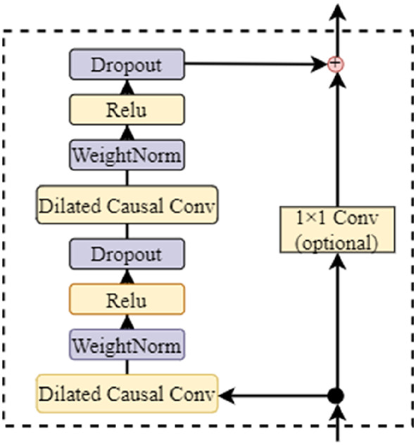
The structure of single residual block.

Another notable feature of TCN is its utilization of dilated convolutions. By inserting “gaps” between the kernel elements, it manages to enlarge the receptive field while keeping the kernel size intact. The following Fig. 4 illustrates the dilated causal convolution. The mathematical formula is as follows:

5

Fig. 4.

The structure of dilated causal convolution.

where y_t and w_k are the output result and weight matrix of the dilated causal convolution structure respectively, x_t−d×k is the sequence information input into the dilated causal convolution structure, and d is the expansion rate.

DCEFormer

The DCEFormer is mainly composed of dual-channel encoder layer and decoder layer. In the encoder, a dual-channel feature decoupling learning mechanism is proposed in the encoder design. As shown in Fig. 5, dual-channel encoder accepts information from the position embedding layer and BiLSTM for processing, and then builds the encoder layers of sensor and timestep, which plays a huge role in improving the degraded information weight allocation of Transformer. The sensor encoder layer realizes the extraction of sensor feature degradation patterns and dynamic weight allocation, while the timestep encoder layer enhances the ability to capture multi-scale temporal dependencies. Finally, an adaptive feature fusion mechanism is designed.

Fig. 5.

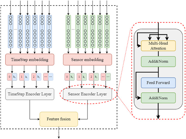
The structure of dual-channel encoder.

Specifically, the dual-channel encoder enables the feature processing results of sensor channel and timestep channel to be independently processed through the weighted attention mechanism, thereby obtaining two output matrices F_t and F_s that are not affected by each other. Then, the processed matrices are fused to obtain a matrix representing the deep feature information.

The encoder architecture comprises dual pathways for sensor and timestep feature extraction, both integrating two core components: multi-head attention mechanism and position-wise feed-forward module (FFN)³². To address training challenges in deep networks, we employ the architecture of Add & Norm to stabilize the gradient flow and accelerate convergence³⁸. This dual-channel design enables independent processing of sensor-wise and temporal dependencies without cross-interference, as illustrated in (Fig. 6).

Fig. 6.

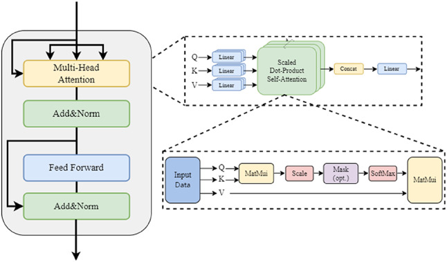
The encoder structure of the transformer.

Sensor encoder layer

We define the CBM sample of the turbofan engine as X = {x₁, x₂, …, x_t, …, x_n}, x_t denotes the data collected by the sensor at time t, and n is the maximum time step. x_t = (x_{1, t}, x_{2, t}, …, x_{k, t}, …, x_{m, t}), x_{k, t} denotes the value of the k channel at time t, and m is the number of channels. The sensor encoder workflow according to (Fig. 5). Firstly, the data processed by BiLSTM and the positional embedding layer are linearly projected through three weight matrices to generate query, key, and value vectors.

6

Since the sensor features of the sequence data are extracted from the sensor dimension, we calculate the attention scores between each sensor element and other sensor elements through matrix multiplication. Therefore, the Q_s, K_s, and V_s can be regarded as matrices composed of vectors. This matrix-based representation helps to efficiently implement operations such as the attention mechanism in a parallel computing environment. In this structure, the most fundamental core is to calculate the weights ɑ_t of different sensors. ɑ_t is obtained by computing the dot product of Q_s and K_s. Moreover, in order to stabilize the gradient and avoid the risks caused by overly large inner products, we perform a reduction by. Finally, applying softmax to the derived matrix yields learnable weights ɑ_t. These learnable weights enable adaptive feature selection, effectively suppressing noise interference in multivariate sensor data streams, as shown in Eq. (7). Then, we multiply V_s by ɑ_t to obtain the attention matrix, which enhances the correlations among the degraded features of the sequence and extracts a more abstract representation of sensor features, as shown in Eq. (8). Meanwhile, we also adopt the multi-head self-attention mechanism which capture complementary contextual features from diverse representation sub-spaces during sequence encoding, as shown in Eq. (9).

7

8

9

where D_model is the input dimension, softmax normalizes a vector of values to a vector of probability distributions that sum to one, W_s is the weight matrix that can be trained by the sensor encoder, Q_s, K_s, V_s are the query matrix, key matrix and value matrix processed by the sensor encoder, and Attention_sensors is the different sensors features obtained by weighted processing by the sensor encoder.

Timestep encoder layer

For exploring the important values contained in different time series, we focus on the dimension of time step and design the timestep encoder layer to automatically focus on the time step characteristics that carry more crucial degraded information. The timestep encoder layer adopts the same structure as the sensor encoder layer. While maintaining the residual connection and the core component of layer normalization, it achieves the feature decoupling in the time dimension through the temporal causal constraint module. Compared with the sensor encoder layer, the timestep encoder layer has its own unique features. Below is the calculation process we carried out on the timestep encoder layer, we transpose X to the input data processed by the BiLSTM and the position embedding layer, which we define as X_t^′, and let the timestep encoder analyze and extract features from the transposed time step data information. Query matrix Q_t, key matrix K_t and value matrix V_t are obtained according to the procedure of (Fig. 5).

10

Meanwhile, in the timestep encoder layer, we also adopted multi-head self-attention mechanism to calculate the weight scores for sensor features at different time steps. This enabled the model to jointly focus on different time step sub-spaces at different positions, thereby improving the prediction performance. Attention_timesteps and F_t can be expressed as:

11

12

where D_model is the input dimension, softmax normalizes a vector of values to a vector of probability distributions that sum to one, W_t is the weight matrix that can be trained by the timestep encoder, Q_t, K_t, V_t are the query matrix, key matrix and value matrix processed by the timestep encoder, and Attention_timesteps is the different timestep features obtained by weighted processing by the timestep encoder.

Feature fusion

After the input sequence X has undergone the feature extraction by the two independent encoder layers mentioned above, it has obtained the features in the time dimension and the spatial dimension. Then, we fuse these two matrices which contain different feature distributions. To ensure the low computational complexity of the model, we adopt an attention-based adaptive feature fusion method. This method performs average pooling on the global features to retain the overall statistical information of the features, while allowing the model to dynamically adjust the contribution of different feature sources, avoiding the additional introduction of positional deviations. Finally, the original feature structure is preserved through the concatenation operation. The details are as follows:

13

14

where Concat (·) represents the concatenation operation, g represents the average pooling of global features, α represents the normalized weight, F_d represents feature fusion matrix, F_s and F_t are calculated from the sensor encoder and the timestep encoder module.

Decoder

In the DCEFormer, the architecture design of the decoder has some similarities with that of the Transformer. Firstly, there is a causal masking mechanism. Before performing the softmax calculation of the attention weights, if the query matrix Q focuses on the key matrix K and value matrix Q of the “future time series”, then the model will suffer from severe overfitting during training. To prevent information leakage during model training and to maintain the autoregressive constraint in sequence prediction tasks, a masking matrix is introduced in the self-attention calculation of the decoder structure. The upper triangular part of the matrix is set to negative, indicating that the relevant fractions of the future time series are not accepted by the model. Secondly, there is the encoder-decoder attention module. Its function is to ensure that the decoder can receive the keys and values processed by the encoder, enabling the decoder to flexibly and dynamically adjust the context information during the generation process, effectively alleviating the problem of truncated long-term sequence dependency caused by the limited receptive field of traditional RNN. Thirdly, there is FFN module which is the output layer of predicted RUL.

Since RUL prediction is a multi-step time series prediction, it usually predicts the future RUL based on the current and past operating conditions of the sensors. Therefore, this paper employs the rolling method for RUL prediction. It can adapt to dynamic data changes and update the model by using the continuously updated RUL prediction values, yielding more accurate and practical results. The Algorithm 1 presents the pseudocode of DCEFormer.

Algorithm 1.

The pseudocode of DCEFormer.

Experiments and analysis

Problem description

Since it is difficult to establish a physical model for complex industrial systems, a reasonable solution is to allocate the expected output as the actual remaining time before the functional failure²⁴. During the operation of aircraft engines, sensors collect a large amount of CBM degradation data that reflects their operational status. Assuming X_k ∈ R_m, k = (1, 2, ., n), where k is the time step and m is the number of sensors. It is expressed as follows:

15

where, X_k is the degradation information of aircraft engines during operation, Y_k is the predicted RUL of the aircraft engines at each time step, and f is proposed that learns the relationship between Y_k and X_k, thereby establishing a mapping function in this paper.

Dataset

Our prognostic model is evaluated on the NASA-developed Commercial Modular Aero-Propulsion System Simulation (C-MAPSS) benchmark dataset³⁹. The dataset provides multivariate temporal sequences that realistically capture both nominal operational profiles and fault-induced transient patterns across complete operational cycles and comprises four distinct subsets (FD001-FD004) with progressively complex fault modes and operational conditions, each containing three core components: training sets, testing sets, real RUL labels. The detailed specifications are systematically summarized in (Table 1).

Table 1.

Overview of C-MAPSS dataset.

Subsets	FD001	FD002	FD003	FD004
Training engines	100	260	100	249
Testing engines	100	259	100	248
Operating conditions	1	6	1	6
Fault modes	1	1	2	2

The training sets contain the engine status parameter information collected by the equipment from its start of operation to the failure cycle. The testing sets contain the data of equipment service life during non-fault periods. In these subsets, both the training sets and the testing sets are composed of 26 feature dimensional. The first two columns record the engine ID and operating cycles of this engine, three to five columns represent various operating parameters of engine, and the remaining 21 feature dimensions are the degradation information captured by different sensors⁴⁰. The sensor visualization is shown in Fig. 7. Since the RUL data of sensors 1, 5, 6, 10, 16, 18 and 19 have no obvious trend of degradation, we delete them and select the remaining 14 sensor data for RUL prediction.

Fig. 7.

The data collected by the sensors.

Experimental preparation

Preprocessing

Normalization: Given that the range magnitudes of individual data channels vary, in order to eliminate the potential influence and errors that might occur in the prediction process, this study uses the following formula to normalize each data channel to the range of [0,1], specifically, for the data X_t = {x₁, x₂, …x_t, …, x_n} are normalized using the following formula:

16

where max (X_t) and min (X_t) denote the maximum and minimum values of data within each channel, respectively.

Sliding window processing: Through the application of sliding window, raw data can be systematically partitioned into overlapping segments of data, which can make the model capture temporally-aware feature representations with increased dimensionality. By this way, the model can fully exert its processing ability for long-term dependencies when dealing with deteriorated information. Through our research, we discovered that setting its length to 40 could yield the best prediction score. The corresponding principle are shown in Fig. 8 (with the sliding stride of 2). We conducted relevant experiments later to verify this finding. The corresponding results are presented Fig. 14.

Fig. 8.

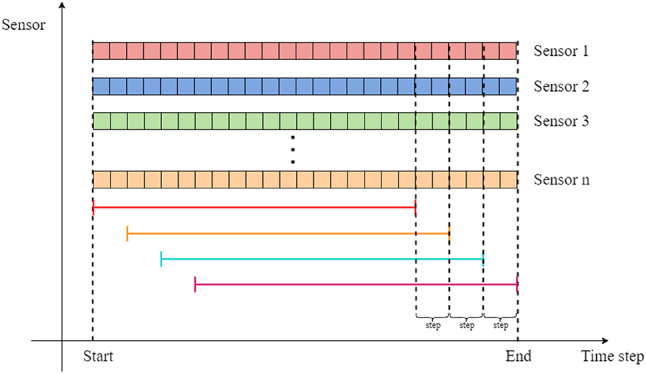
Sliding window.

Statistical properties: Because the degradation process of the engine is dynamic and changing, we use statistical features (such as mean and regression coefficients) to establish this non-linear mapping relationships in predictive model⁴¹. Among them, the mean can reflect the global central tendency and also suppress the interference of noise when the time series fluctuates, helping us study the differences between different time periods of the sequence. And the regression coefficient can quantify the relationship and dependency of different time steps, thereby explaining the potential patterns.

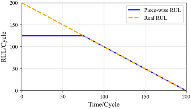
RUL label setting: Based on actual operational condition analysis, the attrition of the engine’s lifespan during the healthy stage can be disregarded. This implies that the lifespan of the engines in the initial stage shows almost no significant change. When their usage reaches the predefined critical point, the engines start to deteriorate until their RUL reaches zero. At this point, the engines are in a state of functional failure. For the engine degradation threshold and the degradation process, in this paper, we use the piece-wise linear function is used to set RUL labels²⁴ as shown in (Fig. 9). Meanwhile, this study sets the RUL to 125. The piece-wise linear function looks like this:

17

Fig. 9.

Rul label setting.

where r_max is the cut-off threshold of the RUL piece-wise linear function, and t_max is the cut-off time point of the RUL piece-wise linear function, t ∈ {1, 2, …, M-T, M-T + 1}.

Evaluation index

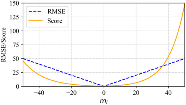
To evaluate the proposed algorithm, two complementary metrics are adopted: the score and the root mean square error (RMSE)⁴¹. As shown in Fig. 10, their combined application provides a balanced assessment of prediction performance—where RMSE quantifies global error magnitude, while Score explicitly incorporates risk sensitivity through asymmetric penalty design. Specifically, Score formula assigns distinct scaling factors to under-prediction and over-prediction scenarios. This asymmetry reflects the aviation industry’s risk-averse stance toward engine failures: overestimating RUL (real RUL < predicted RUL) incurs heavier penalties, as delayed maintenance could escalate catastrophic risks. However, the operational health of the engine is uncontrollable. Sometimes, isolated predictive anomalies (such as excessive deviation of RUL) may occur, which could distort Score. Therefore, combining RMSE can mitigate the risk of misjudging the maintenance strategy based solely on the fluctuation of Score. This dual-index framework ensures the dual advantages of RUL assessment in terms of operational safety and statistical robustness. The Score and RMSE formulas are defined as follows:

18

19

Fig. 10.

Comparison of different error values between score and RMSE metrics.

where , represents the number of samples in the dataset, and represent the predicted RUL and the true RUL of the i-th sample, respectively.

Hyperparameter settings and experimental environment

In order to obtain the optimal hyperparameters of the model, we conducted a grouped cross-validation experiment and used the grid search method to optimize the hyperparameters. To prevent data leakage and avoid affecting the evaluation of the model, in the group cross-validation experiment, this paper divides according to engine units. For all samples in the training set, 80% of them are set as the training subset, and the remaining 20% are set as the validation subset. The testing sets is used separately for the model’s inference. The obtained hyperparameters are listed in (Table 2).

Table 2.

Hyperparameter setting.

	Hyperparameter	Value
BiLSTM	Number of layers	1
	Hidden size	32
	Dropout	0.05
	Activation functions	Tanh
TCN	TCN layers	2
	Kernel size	3
	Dropout	0.1
	Activation functions	Relu
DCEFormer	Sensor encoder blocks	2
	Sensor encoder heads	4
	Timestep encoder blocks	2
	Timestep encoder heads	4
	Decoder blocks	1
	Decoder heads	4
	Activation functions	Softmax
Other	Adam learning rate	0.0005
	Batch size	32
	Fully connected layer activation functions	Relu
	Dropout	0.05
	Early stopping patience	10

The training and testing process is implemented in a 64-bit Windows10 workstation with 32GB of RAM and an Intel i9-9000KF CPU using PyTorch 1.10.1 and python 3.9 to evaluate the effectiveness of the model compared to the state of the advanced RUL prediction methods and to verify the advantages of the model design.

Experimental analysis

Comparison with other experimental methods

In this study, three benchmark methods were adopted for comparative experiments on the benchmark dataset to verify the performance of our model. The first one is the traditional benchmark method including recurrent or convolutional neural architectures, such as BiLSTM and DCNN, etc.; the second one is the hybrid architecture benchmark method including attention mechanisms, such as BiGRU-AS and Deep & Attention, etc.; the third one is the Transformer architecture benchmark method, such as LSTM-Attention, DAST, TATFA-Transformer, GA-Transfomer, DLformer and Dual-Attention, etc.

Tables 3 and 4 respectively present the experimental results of various methods collected on the benchmark subset. The last row of the tables represents our proposed model. Bold font and asterisk font are used to indicate the best result and the second-best result on this subset respectively. The slash symbol indicates missing values. The results show that our model performs more outstandingly on FD002 and FD003, which are the two complex subsets. Especially on the FD002 subset, the reasoning effect of our model is significantly better than that of other models in the two metrics of RMSE and Score. For instance, compared with the existing models, our model has reduced the score indicators by 13.23% on the FD002 subset and 6.83% on the FD003 subset. Regarding another metric, RMSE, the experimental results of our model on the FD002 subset have decreased by 5.91% compared to the existing models. These results indicate that for the RUL prediction problem of complex multivariate time series data, our model demonstrates excellent modeling performance and application prospects.

Table 3.

Comparison of RMSE.

Method	RMSE
	FD001	FD002	FD003	FD004
BiGRU-AS42	13.68	20.81	15.53	27.31
LSTM-Attention43	14.54	/	/	27.08
Deep & Attention44	12.98	17.04	11.88	19.54
DCNN25	12.61	22.36	12.64	23.31
BiLSTM45	13.65	23.18	13.74	24.86
DATCN46	/	15.95	/	18.64
DAST47	11.43	15.25	11.32	18.36
TATFA-Transformer33	12.21	15.07*	11.23*	18.81
DLformer34	/	15.93	/	15.86
GA-Transfomer48	11.63*	15.99	11.35	20.15
Proposed	12.26	14.18	11.19	18.15*

Table 4.

Comparison of score.

Method	Score
	FD001	FD002	FD003	FD004
BiGRU-AS42	284.00	2454.00	428.00	4708.00
LSTM-Attention43	322.44	/	/	5649.14
Deep & Attention44	282.00	1386.00	222.00	2472.00
DCNN25	273.70	10412.00	284.10	12466.00
BiLSTM45	295.00	4130.00	317.00	5430.00
DATCN46	/	1158.93	/	1806.75
DAST47	203.15	924.96*	154.92*	1490.72
TATFA-Transformer33	261.50	1359.70	210.21	2506.35
DLformer34	/	1283.63	/	1601.45
GA-Transfomer48	215.00*	1133.00	228.00	2672.00
Proposed	220.75	802.56	145.12	1573.65*

Compared with the RUL prediction models based on Transformer, our model shows that except for the Score index of FD004, it indicates that considering the time step channel and sensor channel in our model can improve the prediction performance of the model. It is worth noting that DLformer has a poor model performance due to the increase in the number of parameters caused by the use of the feature reuse layer. Although TATFA-Transformer captures the features of the spatial and temporal dimensions through the attention mechanism, this method ignores the processing of local features, resulting in a decrease in the prediction accuracy of the model. Although the DATCN based on the dual-attention mechanism integrates TCN for RUL prediction, its performance cannot be verified in scenarios involving multiple concurrent faults.

Through multi-dimensional index comparison, it can be found that the model with the attention mechanism significantly outperforms the traditional sequence model in terms of prediction accuracy. This verifies the important role of the attention weight allocation mechanism in multivariate time series modeling through dynamic calibration of feature importance, effectively enhancing the representation learning ability of the benchmark model. Notably, BiLSTM demonstrates an architectural advantage over the unidirectional RNN model in sensor channel correlation modeling with its unique gating mechanism and bidirectional information flow design. Further analysis reveals that in the hybrid architecture model, the algorithm adopting dual-channel attention (synchronously optimizing the correlation features between sensor channels and time dependency) has a significant improvement over the unidirectional time series attention model, systematically verifying the assistance of the multi-weight fusion mechanism to the RUL prediction task.

Engine RUL prediction analysis

By comparing the actual trends and predicted trends of engine degradation for all the sub-datasets, as shown in Fig. (11), our dual-channel architecture network can effectively capture the nonlinear degradation dynamics characteristics of the equipment degradation process.

Fig. 11.

The RUL prediction results of all engines in the two testing subsets (a) Prediction results of FD002 (b) Prediction results of FD004.

Subsequently, in this study, a random sampling strategy was adopted to select one engine from each of the four sub-data sets for degradation trajectory analysis. As shown in Fig. 12, it can be seen that the degradation curve fitted by our model is significantly consistent with the actual RUL of the data set, which indicates that our model is competent in predicting the degradation cycle of a single engine. Meanwhile, when the engine enters the decline period, the RUL predicted by our model is less than or close to the actual RUL, which demonstrates the feasibility of our model. Because the harm of late prediction is more serious than that of early prediction in reality, late prediction is prone to cause irreversible disasters, which also indicates that our model performs better in Score than other models. Since the degradation information contained in early prediction is less than that in late prediction, the difficulty of early prediction is also greater, which is the reason for the large error in early prediction.

Fig. 12.

The RUL prediction results of a single engine for each of the four test subsets (a) Engine 58 prediction plot in FD001 (b) Engine 236 prediction plot in FD002 (c) Engine 71 prediction plot in FD003 (d) Engine 68 prediction plot in FD004.

To further determine the distribution of RUL prediction errors for the BLTTNet framework, in this study, the kernel density method was employed to continue the density function of the RUL prediction errors. Figure 13 presents the estimated probability density function and the 95% confidence interval. Both the histogram of the estimation error and the probability density function are concentrated around 0, with the peak located slightly to the left. It indicates that our model has played a role in both early prediction and precise prediction.

Fig. 13.

The error histogram and probability density function of RUL prediction made by BLTTNet. (a) FD001 (b) FD002 (c) FD003 (d) FD004.

Ablation experiment

We validate the effectiveness of our approach by using ablation experiments. The key modules of the model include three modules: BiLSTM, TCN and DCEFormer. We also experimented with the sensor encoding layer and the time step encoding layer of DAST, resulting in the following experiment:

1. No BiLSTM module (w/o BiLSTM).

2. No TCN module (w/o TCN).

3. Sensorless module (w/o Sensor Encoder).

4. Using Serial combination of time series Attention and sensor attention module (serial-attention).

The above method is used to complete the ablation experiment in the FD002 subset, and the RMSE and Score indicators of the proposed model are compared with those of our model. The results are shown in (Table 5), with bold font indicating the best variant.

Table 5.

Ablation experiment of FD002.

Metrics	RMSE	Score
w/o BiLSTM	16.79	1409.31
w/o TCN	16.08	1358.22
w/o sensor encoder	17.19	1523.50
Serial-attention	15.05	1097.25
Proposed	14.18	802.56

The comparison on FD002 subset shows that our model is the best in the performance of RMSE and Score, and also reflects the efficiency of our model in multivariate time series prediction. The w/o Sensor Encoder is essentially an ordinary Transformer experiment, but the results are extremely diverse. This also demonstrates the outstanding performance of DCEFormer in handling features.

Sliding window analysis

The selection of sliding window size critically influences RUL prediction performance when processing multivariate raw time series, as these datasets inherently encapsulate heterogeneous RUL-related information across sensor channels. To systematically investigate this parameter’s impact, we performed comparative experiments on all four C-MAPSS subsets (FD001-FD004) with varying window configurations, as detailed in (Fig. 14). Experimental analysis reveals a non-monotonic relationship between window size and prediction accuracy: (1) For window sizes below 40, both RMSE and Score exhibit progressive deterioration due to insufficient temporal context capture; (2) Beyond the 40-step threshold, although prediction errors show marginal decline, computational complexity escalates quadratically with window expansion. Consequently, through rigorous empirical validation, we identify 40-step windows as the optimal configuration for all subsets, achieving balanced trade-offs between predictive precision and computational efficiency.

Fig. 14.

Model performance for different time window sizes of the dataset (a) RMSE for different factors across time window length (b) Score for different factors across time window length.

Comparison of parameter sizes with other models

In this section, we conducted experiments on the computational complexity of the model. Our model was compared with the transformer-based methods (DAST and DLformer-C). As shown in Table 6, our model performs strongly. For instance, on the FD002 subset, our model demonstrates outstanding performance in both efficiency and accuracy.

Table 6.

Comparison of model performance and efficiency.

Method	FLOPs	FD002		FD004
		Score	RMSE	Score	RMSE
DAST47	5.30 M	924.96*	15.25*	1490.72	18.36
DLfomer-C34	2.26 M	1283.63	15.93	1601.45	15.86
Proposed	1.57M	802.56	14.18	1573.65*	18.15*

Discussion

RUL prediction of complex industrial equipment systems ensures the production and operation efficiency of enterprises, efficient equipment maintenance ability. Our research proposes a fusion framework based on BLTTNet for implementing RUL prediction of multivariate time series, achieving high-precision prediction through a three-level interlinked deep architecture. Firstly, a BiLSTM layer is constructed as the feature extraction layer of time series, fully leveraging the forward and backward state transfer characteristics of this layer to capture the bidirectional temporal feature dependencies, effectively addressing the problem of gradient explosion in LSTM; on this basis, a sensor-timestep dual-channel encoder layer is designed to achieve adaptive feature weight allocation across sensors from different time series, focusing on the critical degradation stages; for the demand of integrating global degradation information, TCN is utilized to extract multi-granularity degradation features and capture the degradation trajectory of the device throughout its life cycle. Finally, this prediction framework represents the probability distribution of the RUL of turbofan engines achieved through the multi-scale feature fusion processed by the model. We analyzed the sliding window size, and ablation experiments further verified the feasibility of the proposed method in time series prediction analysis. Future work will focus more on improving the stability of the model, and further exploration is needed for the real-time nature of the model’s predictions in large industrial fields.

Author contributions

Y.Y.: conceptualization, methodology, validation, writing—original draft preparation, writing—review and editing. C.W. and H.L.: writing—review and editing, conceptualization, supervision, funding acquisition. X.S., H.L., K.F., T.X., and Z.Z.: supervision. All authors reviewed the manuscript.

Funding

This research was funded by Jilin Province Science and Technology Development Plan Project of China (20230201091GX); Jilin Provincial Natural Science Foundation of China (20230101237JC).

Data availability

The datasets generated during and/or analysed during the current study are available from the corresponding author on reasonable request.

Declarations

Competing interests

The authors declare no competing interests.

References

- 1.Zhang, K. & Liu, R. Self-Attention and Multi-Task based model for remaining useful life prediction with missing values. Machines10 (9), 725 (2022). [Google Scholar]
- 2.Guo, Y., Cheng, Z., Zhang, J., Sun, B. & Wang, Y. A review on adversarial–based deep transfer learning mechanical fault diagnosis. J. Big Data. 11, 151 (2024). [Google Scholar]
- 3.Li, X. et al. Energy-Propagation graph neural networks for enhanced Out-of-Distribution fault analysis in intelligent construction machinery systems. IEEE Internet Things J.12, 531–543 (2025). [Google Scholar]
- 4.Cai, Y., Teunter, H., Jonge, B. & R. & A data-driven approach for condition-based maintenance optimization. Eur. J. Oper. Res.311, 730–738 (2023). [Google Scholar]
- 5.Do, P., Assaf, R., Scarf, P. & Iung, B. Modelling and application of condition-based maintenance for a two-component system with stochastic and economic dependencies. Reliab. Eng. Syst. Saf.182, 86–97 (2019). [Google Scholar]
- 6.Shi, Z. & Chehade, A. A dual-LSTM framework combining change point detection and remaining useful life prediction. Reliab. Eng. Syst. Saf.205, 107257 (2021). [Google Scholar]
- 7.Li, X., Li, J., Zuo, L., Zhu, L. & Shen, H. Domain adaptive remaining useful life prediction with transformer. IEEE Trans. Instrum. Meas.71, 1–13 (2022). [Google Scholar]
- 8.Cao, M., Zhang, Y., Hui, J. & Liu, Y. An LSTM-Based approach for capacity estimation on lithium-ion battery. In Proceedings-33rd Chinese Control and Decision Conference, CCDC 2021 494–499 (2021).
- 9.Chan, K. S., Enright, M. P., Moody, J. P., Hocking, B. & Fitch, S. H. K. Life prediction for turbopropulsion systems under dwell fatigue conditions. ASME J. Eng. Gas Turbines Power. 134 (12), 122501 (2012). [Google Scholar]
- 10.Latif, J. et al. Review on condition monitoring techniques for water pipelines. Measurement193, 110895 (2022). [Google Scholar]
- 11.Zhang, Y., Wu, X., Lei, Y., Cao, J. & Liao, W. H. Self-Powered wireless condition monitoring for rotating machinery. IEEE Internet Things J.11, 3095–3107 (2024). [Google Scholar]
- 12.Xu, D., Qiu, H., Gao, L., Yang, Z. & Wang, D. A novel dual-stream self-attention neural network for remaining useful life Estimation of mechanical systems. Reliab. Eng. Syst. Saf.222, 108444 (2022). [Google Scholar]
- 13.Mohr, F., Wever, M., Tornede, A. & Hüllermeier, E. Predicting machine learning pipeline runtimes in the context of automated machine learning. IEEE Trans. Pattern Anal. Mach. Intell.43, 3055–3066 (2021). [DOI] [PubMed] [Google Scholar]
- 14.Shang, Z., Zhang, B., Li, W., Qian, S. & Zhang, J. Machine remaining life prediction based on multi-layer self-attention and Temporal Convolution network. Complex. Intell. Syst.8, 1409–1424 (2022). [Google Scholar]
- 15.Meng, L., Zhao, L., Hao, C. & Zhang, Z. Data-Driven remaining useful life prediction for maritime equipment: a literature survey. In Proceedings-4th International Conference on Autonomous Unmanned Systems, ICAUS 442–451 (2024).
- 16.Sharma, A. K., Punj, P., Kumar, N., Das, A. K. & Kumar, A. Lifetime prediction of a hydraulic pump using ARIMA model. Arab. J. Sci. Eng.49, 1713–1725 (2024). [Google Scholar]
- 17.Zhai, Q. & Ye, Z. S. RUL prediction of deteriorating products using an adaptive wiener process model. IEEE Trans. Ind. Inf.13, 2911–2921 (2017). [Google Scholar]
- 18.Yang, N., Hofmann, H., Sun, J. & Song, Z. Remaining useful life prediction of lithium-ion batteries with limited degradation history using random forest. IEEE Trans. Transp. Electrif. 10, 5049–5060 (2024). [Google Scholar]
- 19.Li, X., Ma, Y. & Zhu, J. An online dual filters RUL prediction method of lithium-ion battery based on unscented particle filter and least squares support vector machine. Measurement184, 109935 (2021). [Google Scholar]
- 20.Shao, H., Jiang, H., Wang, F. & Zhao, H. An enhancement deep feature fusion method for rotating machinery fault diagnosis. Knowl-Based Syst.119, 200–220 (2017). [Google Scholar]
- 21.Shi, J., Gao, J. & Xiang, S. Adaptively lightweight Spatiotemporal information-extraction-operator-based DL method for aero-engine RUL prediction. Sensors23, 6163 (2023). [DOI] [PMC free article] [PubMed] [Google Scholar]
- 22.Sayah, M., Guebli, D., Al Masry, Z. & Zerhouni, N. Robustness testing framework for RUL prediction deep LSTM networks. ISA Trans.113, 28–38 (2021). [DOI] [PubMed] [Google Scholar]
- 23.Liu, Z. et al. A study of a domain-adaptive LSTM-DNN-Based method for remaining useful life prediction of planetary gearbox. Processes11, 2002 (2023). [Google Scholar]
- 24.Babu, G. S., Zhao, P. & Li, X. L. Deep convolutional neural network based regression approach for estimation of remaining useful life. In Proceedings-21st International Conference on Database Systems for Advanced Applications, DASFAA 16–19 (2016).
- 25.Li, X., Ding, Q. & Sun, J. Q. Remaining useful life Estimation in prognostics using deep Convolution neural networks. Reliab. Eng. Syst. Saf.172, 1–11 (2018). [Google Scholar]
- 26.Mitici, M., de Pater, I., Barros, A. & Zeng, Z. Dynamic predictive maintenance for multiple components using data-driven probabilistic RUL prognostics: the case of turbofan engines. Reliab. Eng. Syst. Saf.234, 109199 (2023). [Google Scholar]
- 27.Mao, H., Liu, Z., Qiu, C., Huang, Y. & Tan, J. Prescriptive maintenance for complex products with digital twin considering production planning and resource constraints. Meas. Sci. Technol.34, 125903 (2023). [Google Scholar]
- 28.Guo, R. & Ji, Y. Remaining useful life prediction for bearing of an air turbine starter using a novel end-to-end network. Meas. Sci. Technol.34, 065109 (2023). [Google Scholar]
- 29.Zhu, J., Chen, N. & Peng, W. Estimation of bearing remaining useful life based on multiscale convolutional neural network. IEEE Trans. Ind. Electron.66, 3208–3216 (2019). [Google Scholar]
- 30.Zheng, S., Liu, J., Chen, Y., Fan, Y. & Xu, D. Causal graph-based spatial–temporal attention network for RUL prediction of complex systems. Comput. Ind. Eng.201, 110892 (2025). [Google Scholar]
- 31.Li, X. et al. Adaptive expert ensembles for fault diagnosis: A graph causal framework addressing distributional shifts. Mech. Syst. Signal. Proc.234, 112762 (2025). [Google Scholar]
- 32.Vaswani, A. et al. Attention is all you need. In Proceedings-31st International Conference on Neural Information Processing Systems, NIPS 4–9 (2017).
- 33.Ren, L., Wang, H., Huang, G. & DLformer A dynamic length Transformer-based network for efficient feature representation in remaining useful life prediction. IEEE Trans. Neural Networks Learn. Syst.35, 5942–5952 (2024). [DOI] [PubMed] [Google Scholar]
- 34.Zhang, Y., Su, C., Wu, J., Liu, H. & Xie, M. Trend-augmented and temporal-featured transformer network with multi-sensor signals for remaining useful life prediction. Reliab. Eng. Syst. Saf.241, 109662 (2024). [Google Scholar]
- 35.Wu, Z. et al. Remaining useful life prediction for equipment based on RF-BiLSTM. AIP Adv.12 (11), 115209 (2022). [Google Scholar]
- 36.Liu, C., Li, D., Wang, L., Li, L. & Wang, K. Strong robustness and high accuracy in predicting remaining useful life of supercapacitors. APL Mater.10, 061106 (2022). [Google Scholar]
- 37.Wang, T., Li, B., Fei, Q., Xu, S. & Ma, Z. Parallel processing of sensor signals using deep learning method for aero-engine remaining useful life prediction. Meas. Sci. Technol.35, 096129 (2024). [Google Scholar]
- 38.Liu, L., Song, X. & Zhou, Z. Aircraft engine remaining useful life Estimation via a double Attention-based data-driven architecture. Reliab. Eng. Syst. Saf.221, 108330 (2022). [Google Scholar]
- 39.Li, R. et al. Multiscale feature extension enhanced deep global-local attention network for remaining useful life prediction. IEEE Sens. J.23, 25557–25771 (2023). [Google Scholar]
- 40.Wang, J., Wen, T., Cai, B. & Roberts, C. A high-order strong tracking filter based on a compensated adaptive model for predicting sudden changes in remaining useful life of a lithium-ion battery. J. Energy Storage. 88, 111494 (2024). [Google Scholar]
- 41.Deng, K. et al. A remaining useful life prediction method with long-short term feature processing for aircraft engines. Appl. Soft Comput.93, 106344 (2020). [Google Scholar]
- 42.Duan, Y., Li, H., He, M. & Zhao, D. A BiGRU autoencoder remaining useful life prediction scheme with attention mechanism and skip connection. IEEE Sens. J.21, 10905–10914 (2021). [Google Scholar]
- 43.Chen, Z. et al. Machine remaining useful life prediction via an attention-based deep learning approach. IEEE Trans. Ind. Electron.68, 2521–2531 (2021). [Google Scholar]
- 44.Liu, Y. & Wang, X. Deep & Attention: a self-attention based neural network for remaining useful lifetime predictions. In Proceedings-7th International Conference on Mechatronics and Robotics Engineering, ICMRE (2021).
- 45.Wang, J., Wen, G., Yang, S. & Liu, Y. Remaining useful life estimation in prognostics using deep bidirectional LSTM neural network. In Proceedings-2018 Prognostics and System Health Management Conference, PHM (2018).
- 46.Liu, C., Zhang, L., Yao, R. & Wu, C. Dual Attention-Based Temporal convolutional network for fault prognosis under Time-Varying operating conditions. IEEE T-IM. 70, 1–10 (2021). [Google Scholar]
- 47.Zhang, Z., Song, W. & Li, Q. Dual-aspect self-attention based on transformer for remaining useful life prediction. IEEE Trans. Instrum. Meas.71, 1–11 (2022). [Google Scholar]
- 48.Mo, H. & Iacca, G. Evolutionary neural architecture search on Transformers for RUL prediction. Mater. Manuf. Process.38 (15), 1881–1898 (2023). [Google Scholar]
Associated Data
This section collects any data citations, data availability statements, or supplementary materials included in this article.
Data Availability Statement