The heterogeneous impacts of widespread upzoning: Lessons from Auckland, New Zealand

Abstract

Zoning reform is increasingly recognised as an important strategy to increase housing affordability and environmental sustainability. Few cities have undertaken significant upzoning of low-density neighbourhoods, making the 2016 Auckland Unitary Plan (AUP) probably the most ambitious zoning reform in the world. Parcels zoned for single houses previously dominated Auckland, but three-quarters of them now allow multiple units. Existing studies have documented the building boom that followed this zoning reform, yet the relatively rare case offers additional insights. In this article, we use appraisal, census and zoning data on over 200,000 parcels in Auckland to answer three research questions about the heterogeneous impacts of the AUP. First, to what extent did upzoning increase the appraised value of properties’ redevelopment options? Second, did upzoning increase appraised property values to a greater degree in higher-income and more centrally located neighbourhoods? Finally, was zoning reform in Auckland significantly influenced by similar political pressures as in other countries? That is, was upzoning less likely (and downzoning more likely) in higher-income neighbourhoods? The answers to these three questions are substantially, it’s complicated, and yes.

Introduction

In 2021, New Zealand made international news when it adopted a national zoning reform. Three or more houses would now be allowed on plots of land previously restricted to a single house (Corlett and Cassidy, 2021). The national law was modelled in part on the Auckland Unitary Plan (AUP), adopted in New Zealand’s largest urban area in 2016. The AUP upzoned the vast majority (75%) of its single-family zoned parcels to allow at least three housing units, which resulted in a building boom, especially of townhomes, often at higher densities than previously allowed (Greater Auckland, 2022).

Understanding the impact of Auckland’s 2016 zoning reform is internationally important because there are so few cases of such a widespread change to low-density restrictions. Moreover, the increase in potential building size and parcel coverage in Auckland was considerable, because the city previously prohibited multi-unit housing on a majority of its urban land (Hirt, 2013). Until now, the most well-known cases of low-density zoning reform in the United States (in Minnesota and California) have not substantially increased the permitted size of new structures, limiting the impact of allowing more units per lot (Fox, 2022; Kuhlmann, 2021). Existing research from New Zealand illustrates the overall positive property value and housing production impacts of the AUP (Greenaway-McGrevy and Phillips, 2021; Greenaway-McGrevy et al., 2021) and recent adjustments to the AUP to increase supply closer to employment (Coughlan, 2022).

There is still much to learn from the case of the AUP, especially about the heterogeneity of its impacts. In this article, we use this policy change to test three hypotheses. First, we examine whether the upzoning led to land value appreciation because of the redevelopment options it created, by testing the value impact of greater increases in allowable density. In theory, land value increases reflect the value of an option to add more housing to a parcel. Unlike prior research, which measures the option value of a parcel with a ratio of the value of the structure to total property value (Greenaway-McGrevy et al., 2021), we use a measure we refer to as residual floor area, which measures a parcel’s development potential based on subtracting the built floor area of a parcel from the potential FAR under the zoning regulations. This measurement complements the test of upzoning’s impact.

Second, we examine heterogeneous impacts of the AUP upzoning across neighbourhoods. We hypothesise that upzoning in higher-income neighbourhoods generated larger land value appreciation than in lower-income neighbourhoods, and that parcels in more centrally located neighbourhoods had higher price appreciation if upzoned. Assumptions about the impacts of widespread upzoning on different types of neighbourhoods have hindered productive policy debates, making the answer to this question important.

Third, we are interested in understanding the spatial variation of the upzoning under the AUP as an outcome. Given existing research on opposition to zoning reform, and to accurately frame this case, we test the hypothesis that the Auckland government was more likely to preserve low-density rules in more affluent, older neighbourhoods. One feature of Auckland’s local government structure makes the political economy especially interesting. In 2010, the eight territorial authorities were combined into a single Auckland Council with 21 local boards. Because the new Auckland Plan was published after this consolidation (Auckland Council, 2019: 65), it did not face the complications of multiple jurisdictions acting in competition with one another. Moreover, the central government had charged the new authority to develop a spatial plan. Nonetheless, not all low-density zoning was changed.

Our research strategy is to exploit the change in upzoning policy as a quasi-experiment. We use a ‘repeat appraised property value’ approach with data on over 300,000 properties from before and after the zoning reform for the same parcels to test the first two hypotheses. One benefit of using appraised property values rather than transaction prices is avoiding sample selection bias. Furthermore, appraised values allow larger sample sizes, which can more easily capture the heterogeneous impacts of upzoning. We also discuss the limitations of using this data source.

Our findings confirm that the impact of upzoning under the AUP operates through increasing redevelopment options. We find that the value of a parcel’s residual floor area increased by four to six times depending on the density level to which it was rezoned above a single house. Second, we find that neighbourhood incomes and the distance to the city centre do shape the impacts of upzoning, although not in a simple linear manner. Upzoning under the AUP apparently had the largest impact on middle-income neighbourhoods. Finally, we find that the AUP was less likely to upzone parcels and more likely to downzone parcels in higher-income neighbourhoods, consistent with political pressures in other places.

The article is organised as follows. We first describe the Auckland case, including the consolidation of the planning authority and the creation of the AUP. We then review the research literature on the impacts of upzoning, highlighting the limitations of existing cases available for study. Then, we describe the data and methods we use to answer our questions about how upzoning relates to property valuations and where the upzoning occurred. Finally, we present and discuss the results of our analysis and conclude with suggestions for future research in New Zealand and beyond.

Background of the AUP

Throughout the 20th century, New Zealand’s national government attempted various reform efforts to consolidate Auckland’s multiple territorial and special authorities, with the goal of unified governance for the region. In 2007, New Zealand’s Labour government established a Royal Commission on Auckland Governance, which proposed a single regional government with an elected mayor and six council districts. This new Auckland Council was created and installed in 2010, with a major goal being a unified planning strategy. (For more on the politics and history of the amalgamation, see Asquith et al., 2021a.)

In 2016, after several drafts and public comment periods, the new government council enacted the AUP, which increased allowed densities substantially across most of the metropolitan area. With the target of building over 400,000 dwellings over the next three decades (Auckland Council, 2021a: 5 B2), the AUP created the potential for 18% growth in the city’s main urban area (Auckland Council, 2017).

The proposed AUP 2013

The initial proposal for the AUP in 2013 (Auckland Council, 2013) identified eight issues of regional significance for resource management in Auckland. They included, among others, enabling quality urban growth and enabling economic well-being. One strategy was to increase the housing supply to meet demand, expand housing choices and improve housing affordability. Its objective was to provide a diverse range of housing choices for households and communities to meet their varied needs and lifestyles by:

1. providing ‘a range of residential zones that enable different housing densities, a variety of housing opportunities and different housing types that are appropriate for the existing and planned infrastructure, natural environment and the existing and planned residential character of the area’;

2. enabling an existing dwelling to be converted into two, in specific zones, in a manner that provides high-quality internal and on-site amenities; and

3. requiring resource consent for subdivision and housing development for additional residential land capacity.

The plan introduced four residential zones, the Single House (SH), Mixed Housing Suburban (MHS), Mixed Housing Urban (MHU) and Terrace Housing and Apartment Buildings (THAB), to provide for a variety of densities. The highest density of development is allowed in close proximity to the rapid and frequent service network and within and around centres. Only one two-storey unit per lot is permitted in the SH zone, the two Mixed Housing zones allow three units (in two and three storeys) and the THAB zone does not limit the number of units allowed within five storeys. The zones increase in permissible floor area ratio (FAR) and height.

Figure 1 is a map showing the zone types by neighbourhood. We note that although the AUP upzoned the majority of the SH zones to allow higher-density development, many SH zones remained – especially in older neighbourhoods near the city centre. Moreover, we also observe that higher-income residents are concentrated in lower-density zones (SH and MHS). Eighty per cent of the highest income group (with a median annual personal income of more than NZ$50,000) lived in these two lower-density zones, not the MHU and THAB zone. Appendix B provides maps showing median incomes and median housing values by neighbourhood for context.

Figure 1.

Map of the four major residential zones in the Auckland Unitary Plan.

Source: Adapted from Auckland Council (2022).

Related literature

The connection between restrictive land-use rules and high housing prices is well established on both the metropolitan (Glaeser and Gyourko, 2017; Saiz, 2010) and sub-metropolitan scale (e.g. Kok et al., 2014), although less research has focused on the supply-side mechanism for this price impact (for a literature review, see Manville et al., 2020; Monkkonen et al., 2020b). Advocates have used this body of empirical evidence to support zoning reforms and increase permitted densities, perhaps most famously in California, where the state government recently allowed two units per lot and gave single-family homeowners the ability to split lots (Dougherty, 2021).

Most studies on the topic find that new housing production reduces rents and prices (Phillips et al., 2021). Research by Asquith et al. (2021b), Pennington (2021) and Li (2021), for example, finds that new market-rate housing production is associated with a decrease in rents. In part, this occurs through a ‘chain of moves’ (part of the filtering process) when new housing is built, as it creates indirect but relatively immediate benefits for low-income households (Bratu et al., 2023; Mast, 2019). These studies follow individual units through several residential moves, identifying who moves into the units that are vacated by people moving into new buildings, who moves into the units those people left and so on. Following a chain of moves in Helsinki, Finland, Bratu et al. (2023) find that 10% of residents in new market-rate units move from neighbourhoods in the bottom quintile of the income distribution but that 30% of residents move out of bottom-quintile neighbourhoods when they trace the chain five moves back.

Housing market filtering has a long research history. Sweeney (1974) established the foundation for theoretical models of housing filtering. Brueckner (1980) extended the classic circular city model to allow properties to move between high-income and low-income occupants in examining the housing filtering process. Bond and Coulson (1989) then investigated a filtering model in which the neighbourhood experiences an externality associated with tenants’ wealth. Empirically, Brueckner (1977) and Phillips (1981) used data to demonstrate the determinants of a census tract’s eligibility for residential succession to confirm the housing filtering process. However, this study, amongst many others, only searched for results consistent with filtering rather than directly examining individual units’ filtering effects.

The recent study by Rosenthal (2014) provided the first direct empirical evidence of filtering by estimating repeat income models based on new occupants of the same house for both owner-occupied and rental housing. Rosenthal (2014) used a constant quality repeat income index model and a structural model of housing demand to theorise filtering rates in the housing market as a function of depreciation and the change in house prices. Building on Rosenthal (2014), Liu et al. (2022) estimated filtering rates at geographically and temporally disaggregated levels for owner-occupied properties and showed that filtering rates for owner-occupied, single-family houses vary widely across and within metropolitan statistical areas (MSAs) and across time in the United States.

In spite of recent progress, questions remain about the impacts of zoning reform (Schill, 2005), in part because there are few cases of widespread upzoning to study (Dong, 2021; Freeman and Schuetz, 2017). In most instances, zoning changes only apply to specific parcels or small areas, often referred to as spot upzoning (Gabbe, 2019). In contrast, widespread or broad upzoning is theorised to have different price and supply effects than spot upzoning, as it reduces the relative value of parcels zoned for higher density by creating many of them (Monkkonen, 2019; Phillips, 2022). The distinction is vital for policy discussions. Even when scholars emphasise the limitations of findings from their studies on spot upzoning for discussions about broad upzoning, as Freemark did in his study on Chicago’s zoning changes near transit stations, advocates and policymakers opposed to zoning reform still misuse them in discussions about broad upzoning.¹

Another challenge of projecting the impacts of broad upzoning using cases of spot upzoning is illustrated by the study of upzoning in a transit-oriented development programme connected to a new rail line in Phoenix, Arizona (Atkinson-Palombo, 2010). The study found that values increased in neighbourhoods with mixed-land use much more than in primarily residential neighbourhoods. This reflects the complication of this case, as the programme upzoned near station areas, but the rail line was new, and there were many concurrent expectations about neighbourhood changes.

In the remainder of this literature review, we highlight three pending questions for the literature to which our study contributes. The first builds on one of the two existing studies on Auckland’s zoning reform, which focuses on the impacts on property values and the redevelopment option (Greenaway-McGrevy et al., 2021). In addition to the positive correlation between the level of upzoning and property values, Greenaway-McGrevy et al. (2021) tested the differential impacts of upzoning on sites with more or less potential for redevelopment, motivated by real options theory (Clapp et al., 2012). They measured a parcel’s development intensity as the ratio of the structure value to total property value and found that properties with lower levels of development intensity appreciate more. For example, houses located in Zone 4 appreciated by 15% if their initial intensity was 0 and only 9% if the intensity was 1 (Greenaway-McGrevy et al., 2021: 969). They also found that upzoning had a depreciative effect on high-intensity parcels – dwellings for which the structure was the majority of the property value actually saw prices decline relative to those for which land was the majority of the property value.

Our study builds on this existing work by developing a measure of a parcel’s development potential based on a parcel’s allowed floor area ratio beyond what is already built there rather than value ratios. We consider that this allows us to more directly measure the impact of a change to zoning. This also allows us to test how much the magnitude of entitled density increase matters.

The second question is how upzoning impacts different types of neighbourhoods. Because the change in value reflects development possibilities, it is expected to depend on the demand for denser development on a parcel. Many empirical studies on the upzoning place too little emphasis on the role of demand. Demand for housing units of different sizes and configurations varies across neighbourhoods. Thus, increasing permitted density levels in a far-flung suburb, for example, may have a limited impact on values because density restrictions are not binding constraints to development there. In contrast, values of centrally located parcels for which low-density rules prevent high-density redevelopment will change. These heterogeneous impacts of upzoning in different neighbourhoods are subject to two forces, that is, the benefits of utilising the additional residual floor area and the costs of the influence on the neighbourhood quality. People living in single-family housing areas would perceive a denser neighbourhood as a negative externality.

In addition, housing stock preferences and levels of income inequality mean that developers will not necessarily build the maximum density allowed in all neighbourhoods. In places with high levels of inequality, where affluent households prefer detached houses, they will be able to outbid even multiple households for land (Monkkonen et al., 2020a). For this reason, we examine the impacts of upzoning on low-density neighbourhoods of different incomes. A priori, we might expect some of the highest-income neighbourhoods to remain low density even after upzoning, given preferences and the ability to pay for large housing units. This will be reflected in part by a differing value of the redevelopment option in neighbourhoods of different incomes.

Understanding the heterogeneous impacts of upzoning across neighbourhoods is also essential for debates over zoning reform. Opponents of upzoning sometimes argue that housing redevelopment in low-income neighbourhoods will lead to their gentrification and induce existing resident displacement (Rodríguez-Pose and Storper, 2019). In California, for example, concern about the displacement of low-income households resulting from a proposed broad upzoning programme in 2018 (Senate Bill 827) led to the creation of a ‘sensitive community’ designation in a subsequent legislative proposal. This proposal, Senate Bill 50, would have exempted low-income neighbourhoods from upzoning (for background and a description of the designation process, see Dougherty, 2020; Hochberg, 2019). Similar issues have also been raised for countries in the Global South (Denoon-Stevens and Nel, 2020). Evidence from Auckland on this point will therefore be useful for the international discussion.

The third question we consider relates to the political economy of Auckland’s zoning changes. We ask whether, as in other parts of the world (Gabbe, 2019), the zoning decisions were influenced by the political power of more affluent and vocal residents (Einstein et al., 2019; Monkkonen, 2016). Local media suggests that Auckland is susceptible to the same issues as other cities (Donnell, 2021). We primarily test the hypothesis that a parcel in a higher-income neighbourhood was less likely to be upzoned and more likely to be downzoned with the use of ‘special character districts’ designations.² In addition, we examine upzoning by the distance to the city centre. Most urban planning theory promotes allowing higher densities near city centres to reduce commute times and encourage sustainability (Jabareen, 2006). This question is important not only to assess whether the Auckland case is completely atypical, but also to frame our results on the prior hypothesis tests.

Data

Our research questions address zoning changes and assessed value appreciation at the individual house or parcel level. In order to assess the correlation between the characteristics of people and parcels and zoning changes, we rely on three datasets.

The first is provided by Relab° (2022). Relab is an industry-leading data platform in New Zealand that offers real-time access to thousands of property data points (https://relab.co.nz/). From this database, we extract the appraised property value (APV) of about 340,000 dwellings from June 2016 to June 2021 (released in 2017 and 2022).³ The database also contains the land area of parcels, the existing floor area of dwellings and the maximum developable floor area based on the zoning code. The change in the APVs reflects, among other factors, the effects of the AUP implemented in 2016. Detailed information on New Zealand’s appraisal system is provided in Appendix A, and further information on the zoning code and the AUP can be obtained at Auckland Council (2021a, 2022).

Using appraised property values gives us a larger sample size than transaction data, as the number of housing transactions per annum accounts for less than 6% of the total number of houses in Auckland. These data also help us avoid selection bias in applying the repeat sales method. Our analysis focuses on houses with freehold and cross-lease (FH/CL) titles, which account for 68% and 17% of the city’s parcels.⁴ We limit our sample to the four residential zoning categories, which account for 34.7% of the city’s parcels, introduced under the AUP previously described in the second section.

Table 1 reports the summary statistics of the variables from Relab’s parcel-level dataset, as well as our control variables. The data on median personal incomes come from our second data source, the censuses of 2013 and 2018 (New Zealand Government, n.d.). We match parcels to neighbourhoods as delineated by the New Zealand Census. The smallest census unit is Statistical Area 1 (SA1),⁵ and there are roughly 8000 in Auckland. The final two control variables are the distance to the city’s central business district (CBD) and a measure of job accessibility.⁶ We calculated these variables based on parcel locations and job data from the New Zealand Census. Auckland remains a relatively monocentric city, and the correlation between our job access measure and distance to CBD is over 0.6. The proximity to the centre matters for more than just access to employment; thus, it is useful to combine this traditional measure of location value proximity to jobs.

Table 1.

Summary statistics of the parcel and neighbourhood data.

Description	Variables	Mean	SD	Min.	Max.
Parcel-level data
Change in value (log ratio between periods 2 and 1)	log(APVi, 2,/APVi, 1)	0.30	0.13	−2.76	3.06
Residual floor area ratio	RFAR i, 2	0.99	0.77	−44.0	18.94
Maximum_subdivisible number of_lots	MAX LOTi	5.53	83.20	1.00	46,909
Distance to central business district (km)	DISi	14.38	10.83	0.84	1196.71
Job accessibility	JOBi	58,953	60,154	1314	295,098
Change in improvement value (log ratio between periods 2 and 1)	log(IVi, 2/IVi, 1)	0.00	0.66	−4.05	6.30
Change in median income (log ratio between periods 2 and 1	log(INi, 2/INi, 1)	0.16	0.21	−1.98	1.89
No. of suburbs		282
No. of freehold (FH) and cross lease (CL)247,742 FH, 94,201 CL
Neighbourhood-level data
Income 2013 (NZ$)		30,795	10,392	3500	85,300
Income 2018 (NZ$)		35,943	10,851	3800	82,800
No. of houses		36	16	1	288
No. of SAIs		7983

Note: Total number of observations is 341,943. Summary statistics are based on house-only parcels of the four designated zone types. log(APV_{i, 2}/APV_{i, 1}) represents the appraised property values (APVs) in year 2021 versus 2016; RFAR_{i, 2} is the residual floor area ratio (RFAR) in year 2021; log(IV_{i, 2}/IV_{i, 1}) is the natural log of improvement value (IV) ratios in years 2021–2016; whereas log(IN_{i, 2}/IN_{i, 1}) is the natural log of median personal income (IN) ratios in 2018 versus 2013.

The third data source is Auckland Council’s district valuation roll (DVR⁷) from 2014 and 2022. This provides housing stock data, including parcel-level zoning designation before and after the AUP came into effect. In this way, we can directly measure the impact of zoning changes on APV change at the parcel level by comparing the zone types before and after the AUP.

Table 2 reports the proportion of properties by zone type in 2014 and 2022. The broad scale of upzoning is illustrated by the drop in the proportion of SH zones from 78% in 2014 to 27% in 2022, and the increase in the share of parcels zoned MHS, MHU and THAB. Even though about 15,000 parcels were downzoned from more permissive zoning to SH, the total number of SH parcels dropped by 66%. In contrast, the total number of MHS-, MHU- and THAB-zoned parcels increased by 387%, 94% and 610%, respectively.

Table 2.

Parcels by zone type in periods 1 (2016) and 2 (2021).

Panel A: Count	Zone, period 2 (2021)
	SH	MHS	MHU	THAB	Total
Zone, period 1 (2016)
SH	38,810	75,263	36,420	8679	159,172 (78%)
MHS	5008	3461	6576	3064	18,109 (9%)
MHU	10,086	8484	4880	1209	24,659 (12%)
THAB	338	1073	80	389	1880 (1%)
Total	54,242 (27%)	88,281 (43%)	47,956 (24%)	13,341 (7%)	203,820
Panel B: Income	Zone, period 2 (2021)
	SH	MHS	MHU	THAB	Average
Zone, period 1 (2016)
SH	33,700	28,300	24,500	25,100	27,900
MHS	37,600	30,500	26,400	27,100	30,400
MHU	38,900	37,400	29,200	27,200	33,175
THAB	38,400	39,600	47,800	29,900	38,925
Average	37,150	33,950	31,975	27,325

Note: The Single House (SH) zone only allows one dwelling per site, with a two-storey building height limit and 35% maximum building coverage; the Mixed Housing Suburban (MHS) zone allows three dwellings per site with a two-storey building height limit and 40% maximum building coverage; the Mixed Housing Urban (MHU) zone allows three dwellings per site with a two-storey building height limit and 45% maximum building coverage; the Terrace Housing and Apartment Buildings (THAB) zone has no restriction on the number of dwellings per site, but a five-storey building height limit and 50% maximum building coverage. The figures in Panel B are the median personal disposable annual incomes in New Zealand dollars of households living within the parcels that were rezoned from period 1 to period 2. Source: Auckland Council (2021a) (H3 Residential - Single House Zone, H4 Residential - Mixed Housing Suburban Zone, H5 Residential - Mixed Housing Urban Zone, H6 Residential - Terrace Housing and Apartment Buildings Zone).

One challenge of this study is combining data from different sources and years. For example, the Relab data on the appraised property values and residual floor areas are based on the latest zoning built in 2021 and the changes in APV between the appraisals in 2016 and 2021. The DVR dataset provides the housing attributes and zone types in 2014 and 2022. The census dataset provides demographic data such as personal income in the 2013 and 2018 censuses. We combine the three datasets using the valuation reference number of the individual property parcel and by joining parcels to SA1 areas to match them to census data, which is a straightforward process.

Analytical approach

Our empirical design treats the upzoning policy change as a quasi-natural experiment to measure the effects of the increase in potential residential development intensity through upzoning. We refer to this change as the residual floor area ratio in period 2 (2021, represented by subscript 2) $\left(RFA{R}_{i,2}\right)$. For the $i$th parcel, $RFA{R}_{i,2}$ is defined as follows:

$$RFA{R}_{i,2}=\frac{MDF{A}_{i,2}-EDF{A}_{i,2}}{EDL{A}_{i,2}}$$ (1)

where $MDF{A}_{i,2}$ is the sum of the maximum developable residential floor area in square metres (m²) of the ith parcel after the upzoning policy change in 2016 (i.e. in 2021 or period 2), $EDF{A}_{i,2}$ is the sum of the existing developed residential floor area in m² of the ith parcel and $EDL{A}_{i,2}$ is the sum of the existing developed residential land area in m² of the ith parcel, all in 2021.

A Repeat-APV model estimates the impact of the RFAR on the change of APV, and mathematically:

$$\begin{gathered} log\left(AP{V}_{i,2}/AP{V}_{i,1}\right)={\alpha }_1+{\beta }_{1}RFA{R}_{i,2} \\ +\sum _{q=2}^4{\beta }_{q}FA{R}_{i,2,q}+{\gamma }_{1}log\left(I{V}_{i,2}/I{V}_{i,1}\right) \\ +{\gamma }_{2}log\left(I{N}_{i,2}/I{N}_{i,1}\right)+{\gamma }_{3}DIS+ \end{gathered}$$ (2)

where $AP{V}_{i,1},AP{V}_{i,2}$ and $I{V}_{i,1},I{V}_{i,2}$ are the appraised property values and improvements values appraised in period 1 (2016) and period 2 (2021) of the ith parcel, respectively. ${\alpha }_1$ is a constant term to measure the overall market house value change in Auckland between the two periods. $I{N}_{i,2},I{N}_{i,1}$ are the median personal incomes in the latest census (2013 or 2018) of the ith parcel’s neighbourhood. $DI{S}_i$ is the distance from the centroid of the ith parcel to the Sky Tower at the city centre in km.

The upzoning policy change is considered a quasi-experiment, and the upzoning effect is estimated by a difference-in-differences (DID) model (Model 2). Neighbourhoods with high income are the control group, and the lower-income neighbourhoods are the treatment groups. The Repeat-APV approach studies the change in APV before and after the upzoning policy change.

Mathematically,

$$\begin{gathered} log\left(AP{V}_{i,2}/AP{V}_{i,1}\right)={\alpha }_1+{\beta }_{1}RFA{R}_{i,2} \\ +{\theta }_{q}RFA{R}_{i,2}\times log\left(I{N}_{i,1}\right) \\ +{\gamma }_{1}log\left(I{V}_{i,2}/I{V}_{i,1}\right)+{\gamma }_{2}log\left(I{N}_{i,2}/I{N}_{i,1}\right) \\ +{\gamma }_{3}DIS+ \end{gathered}$$ (3)

Empirical results and discussion

In this section, we present the results of hypothesis tests of the price impacts of the residual FAR generated by different zoning changes. We also examine variations in price impacts depending on initial zoning considering the moderating effects of neighbourhood incomes and location. Then, we examine the role of neighbourhood income and location in the likelihood that a parcel had its zoning changed.

Table 3 shows the results of the four Repeat APV Baseline Models. We run identical models on the data sub-samples, separated into each zone type in period 2. All four models show a positive association between upzoning and appraised property values. The value of the redevelopment option varies across zones in the hypothesised manner. In more permissive zones, residual FAR is worth more, presumably because more units can be built. In the SH sub-sample, a doubling of the residual floor area ratio from one to two (the average RFAR in the sample is 0.99) is associated with an increase of only 2% in property value, whereas in the zones that permit more density, the coefficients indicate an increase in value of between 8% and 13% when residual FAR is doubled. The results are consistent with the hypothesis that greater levels of upzoning increase value more.

Table 3.

Estimation results of the repeat-APV baseline model for different zones.

Dep. Var. log(APVj, 2/APVj, 1)	MODEL 3a	MODEL 3b	MODEL 3c	MODEL 3d
	SH only	MHS only	MHU only	THAB only
Constant	0.159 (26.64)***	0.180 (49.50)***	0.654 (5.60)***	0.184 (20.58)***
RFARj	0.018 (16.31)***	0.112 (90.05)***	0.084 (48.70)***	0.132 (38.82)***
log(IVj, 2/IVj, 1)	0.101 (129.33)***	0.015 (33.96)***	0.013 (18.70)***	−0.0002 (−0.14)
log(IVi, 2/IVi, 1)	−0.008 (−4.95)***	−0.004 (−2.95)***	0.001 (0.43)	−0.009 (−2.22)**
DISj	−0.0004 (−2.73)***	−0.0002 (−3.71)***	−0.0005 (−5.94)***	0.0001 (0.19)
MAX LOTi	0.001 (16.04)***	0.00005 (5.29)***	0.0004 (17.47)***	0.000 (0.56)
Cross-lease	−0.029 (−32.85)***	−0.093 (−134.25)***	−0.113 (−107.39)***	−0.143 (−72.21)***
Location fixed effect (suburbs)	Yes	Yes	Yes	Yes
Adj R-squared	0.48	0.31	0.30	0.39
No. of obs.	69,996	166,033	78,557	27,357

Note: t-statistics in parentheses. In parcel-level analysis, title type effect, lot subdivisibility effect and location effect are also controlled. Zone type is based on the Relab data.

^***p < 0.01.

^**p < 0.05.

^*p < 0.10.

The coefficient on the structure value ratio in Table 3 in period 2 compared to the structure value in period 1 is much larger (almost 10 times) for SH properties than the others. This reflects the fact that structural rehabilitation plays a much larger role in price appreciation for single-house properties than for other types of buildings.

To simplify our estimations of the impact of zone change on value and address heterogeneity in the nature of upzoning, we separate parcels into four sub-samples based on their initial zone. We then estimate the increase in value for different change categories. Recall from Table 2 in the fourth section that there are 16 possible combinations of zone-type changes between the four zone types we analyse; for example, from low density to medium density or from medium density to high density. In the models presented in Table 4, we also expand our controls to include the measure of job accessibility described previously.

Table 4.

Estimation results of the repeat-APV zone type change model (zone type based on the DVR datasets).

Dep. var. log(APVj, 2/APVj, 1)	MODEL 2a	MODEL 2b	MODEL 2c	MODEL 2d	MODEL 2e	MODEL 2f	MODEL 2g	MODEL 2h
	From SH	From SH	From MHS	From MHS	From MHU	From MHU	From THA	From THA
Constant	0.304 (11.57)***	0.262 (10.10)***	0.189 (7.02)***	0.123 (4.65)***	0.405 (16.94)***	0.310 (12.65)***	0.221 (0.80)	0.201 (0.73)
log(IVj, 2/IVj, 1)	0.001 (1.68)*	0.004 (5.79)***	0.013 (7.68)***	0.014 (8.69)***	0.044 (32.60)***	0.044 (33.05)***	0.151 (20.90)***	0.151 (20.89)***
log(IVi, 2/IVi, 1)	−0.011 (−5.38)***	−0.010 (−5.10)***	0.005 (0.83)	0.013 (2.12)**	0.012 (3.02)***	0.011 (2.58)***	0.063 (2.68)***	0.062 (2.64)***
DISj	−0.0003 (−4.44)***	−0.0003 (−4.54)***	−0.001 (−4.24)***	−0.001 (−3.64)***	−0.007 (−5.41)***	−0.007 (−5.57)***	0.020 (1.44)	0.021 (1.50)
JOBj	2.23 × 10−7 (6.80)***	2.03 × 10−7 (6.29)***	9.64 × 10−8 (0.94)	7.46 × 10−8 (0.75)	8.09 × 10−9 (0.19)	1.26 × 10−8 (0.30)	−5.93 × 10−6 (−5.44)***	−5.89 × 10−6 (−5.39)***
RFARj		0.077 (53.41)***		0.139 (23.49)***		0.045 (16.12)***		0.001 (0.81)
SH→MHS	0.059 (31.47)***	0.069 (37.23)***
SH→MHU	0.079 (31.47)***	−0.042 (−14.62)***
SH→THAB	0.122 (53.52)***	0.041 (15.27)***
MHS→SH			−0.002 (−0.38)	−0.028 (−5.90)***
MHS→MHU			0.015 (5.13)***	−0.218 (−21.03)***
MHS→THAB			0.031 (8.34)***	−0.133 (−16.83)***
MHU→SH					−0.086 (−26.81)***	−0.017 (−3.10)***
MHU→MHS					−0.030 (−12.12)***	0.045 (8.52)***
MHU→THAB					0.003 (0.84)	0.028 (6.51)
THAB→SH							−0.107 (−3.59)***	−0.105 (−3.51)***
THAB→MHS							−0.053 (−1.98)**	−0.051 (−1.91)*
THAB→MHU							−0.004 (−0.16)	−0.004 (−0.19)
MAX LOTi	0.00003 (3.03)***	0.00002 (2.15)***	0.007 (24.64)***	0.006 (20.50)***	0.0002 (3.59)***	0.0002 (2.76)***	−0.007 (−4.18)***	−0.007 (−4.22)***
Cross-lease	−0.080 (−70.91)***	−0.093 (−81.69)***	−0.096 (−32.69)***	−0.110 (−37.55)***	−0.079 (−45.48)***	−0.085 (−48.15)***	−0.039 (−3.03)***	−0.039 (−3.06)***
Location fixed effect (suburbs)	Yes	Yes	Yes	Yes	Yes	Yes	Yes	Yes
Adj R−squared	0.26	0.28	0.31	0.34	0.30	0.31	0.48	0.48
No. of obs.	87,761	87,761	12,115	12,115	21,655	21,655	736	736

Note: t−statistics in parentheses.

^***p < 0.01.

^**p < 0.05.

^*p < 0.10.

Table 4 shows the results of the regression of APV change on zone type change using the Auckland Council 2014 and 2022 DVR data. The results in MODEL 2a confirm the prior estimates of a progressively large, positive effect of upzoning on change in property values. Using the unchanged SH zoned parcels as a reference category, the Repeat-APV Zone Type Change Model shows the strongest upzoning effect of a 12% increase in value for SH parcels rezoned to THAB – the most permissive zoning category. The effects of upzoning to MHU and MHS were also significant and associated with between a 6% and 8% increase in value respectively.

As theory predicts, the upzoning effects of changes between already more permissive zones to higher-density rules, moving from MHS to MHU and THAB, are smaller. The results of between 2% and 3% change are similar to those found by Greenway-McGreevy et al. (2021). Similarly, Kuhlmann’s 2021 study of upzoning single-family zones to threeplexes in Minneapolis found a 3– 5% price impact compared to otherwise similar properties in adjacent municipalities with no price change.

One important finding is that after taking into account the residual floor area ratio (RFAR) in MODEL 2b, the effect of upzoning from SH to MHU is negative. This fits the basic theory, which is that the impacts of upzoning on property value are expected to be found in the development potential but that expectations about neighbourhood change may make the total impact heterogeneous. Upzoning combines the benefits of additional residual floor area as well as any costs of the change in neighbourhood conditions. In MODEL 2b, while the RFAR exhibits a positive effect on appraisal values, the negative 4% effect from the zone change may mean that people perceive a denser neighbourhood as a negative externality.

The results also show a predicted negative relationship between downzoning and property values; for example, parcels that changed from MHU to SH lost 9% of value and parcels that changed from THAB to either SH or MHS lost about 6%.

Income and distance to the city’s CBD

We test a second hypothesis about heterogenous upzoning impacts across neighbourhoods of different income levels in two ways. Table 5 shows the results of the two DID models that regress the changes of APV against RFAR, IN, DIS and controls. They show that the median property value increased by about 16% from July 2016 to June 2021. Second, controlling for the effect of improvement values of structures, neighbourhood incomes and distance to CBD, the positive effects of upzoning on values were moderated by neighbourhood income levels in period 1 and the distance to the city centre of the house. Models 3a and 3b show that the value increase with more RFAR is lower for higher-income neighbourhoods and higher for parcels farther away from the city centre.

Table 5.

Estimation results of the repeat-APV DID models for different income neighbourhoods and DID models.

Dep. Var. log(APVi, 2/APVi, 1)	MODEL 4a	MODEL 4b	MODEL 4c	MODEL 4d	MODEL 5a	Model 5aa	Model 5ab	Model 5ac	Model 5ad	MODEL 5b
	Q1 income group	Q2 income group	Q3 income group	Q4 income group	DID on IN	DID on IN_Q1	DID on IN_Q2	DID on IN_Q3	DID on IN_Q4	DID on DIS
Constant	0.170 (21.35)***	0.034 (7.07)***	0.127 (23.29)***	0.143 (16.86)***	0.153 (49.79)***	0.172 (21.59)***	0.342 (7.16)***	0.128 (23.32)***	0.138 (16.28)***	0.165 (53.25)***
RFAR i, 2	0.072 (47.35)***	0.292 (103.81)***	0.123 (64.58)***	0.028 (25.04)***	0.253 (43.84)***	0.141 (9.57)***	0.523 (12.29)***	0.334 (5.64)***	0.548 (17.73)***	0.073 (84.13)***
RFARi, 2×log(INi, 1)					−0.016 (−29.65)***	−0.071 (−4.72)***	−0.023 (−5.43)***	−0.020 (−3.57)***	−0.048 (−16.85)***
RFARi, 2×DISi										0.001 (31.42)***
log(IVi, 2/IVi, 1)	−0.003 (−3.60)***	0.015 (24.26)***	0.027 (42.91)***	0.063 (87.33)***	0.015 (45.74)***	−0.026 (−3.69)***	0.015 (24.40)***	0.027 (42.91)***	0.064 (88.15)***	0.015 (45.71)***
log(INi, 2/INi, 1)	−0.030 (−15.04)***	−0.018 (−7.72)***	−0.010 (−4.51)***	0.003 (1.20)	−0.014 (−13.76)***	−0.034 (−15.62)***	−0.020 (−8.67)***	−0.011 (−4.85)***	−0.005 (−2.00)***	−0.003 (−2.73)***
DISi	−0.001 (−8.34)***	−0.0002 (−3.10)***	−0.0002 (−2.24)**	0.0003 (1.93)*	−0.0002 (−4.39)***	−0.0010 (−8.34)***	−0.0002 (−3.13)***	−0.0002 (−2.25)**	0.0003 (1.63)	−0.001 (−24.06)***
Adj R−squared	0.33	0.34	0.31	0.34	0.30	0.33	0.34	0.31	0.35	0.30
No. of obs.	83,403	89,255	88,134	81,151	341,943	83,403	89,255	88,134	81,151	341,943

Note: t−statistics in parentheses. Substituting the average incomes of Q1, Q2, Q3 and Q4 at NZ$19,484.05, NZ$27,805.58, NZ$34,472.24 and NZ$45,346.63 respectively into the coefficients of Models 5aa to 5ad. The moderating effect of neighbourhood income level on the RFAR effect on APV is found to be an inverted U-shape from 0.07 of Q1, 0.29 of Q2, 0.12 of Q3 and 0.03 of Q4.

^***p < 0.01.

^**p < 0.05.

^*p < 0.10.

To better understand these relationships, Table 5 also shows the results of the three sub-sampling estimations of the baseline model (Model 4a) for parcels divided into three sub-groups based on average neighbourhood personal income in 2018 – below NZ$30,000, NZ$30,000–38,999 and NZ$39,000 or more. (Each accounts for about 33% of the sample.) The sub-sample results show a non-linear effect of neighbourhood income on the change in values. There is a substantially larger positive relationship between upzoning and APV change for middle-income neighbourhoods, and the effects are the lowest in high-income neighbourhoods. These results invite further research and help explain why the income coefficient measured in the DID model is negative.

It is difficult to contextualise the results with existing research because, to our knowledge, only one other study (Kuhlmann, 2021) has tested this hypothesis. This found that in Minneapolis properties in neighbourhoods below the median house price saw greater price appreciation. However, it divided neighbourhoods into only two groups, above and below median house value.

Zoning change as dependent variable

Finally, we consider the zoning change itself as a dependent variable and test the hypothesis that neighbourhood incomes and location correlate to a parcel’s chance of having its zoning changed by the AUP. We first examine a simple graphical and tabular representation of the data and then use four Probit regression models.

In Figures 2 and 3, we observe patterns of zoning changes by neighbourhood incomes and distances to the city centre. Figure 2 shows the share of parcels zoned SH in periods 1 and 2 at different distances from the city centre. Because the number of parcels did not change substantially (although, to be clear, there are many more parcels at farther distances from the centre), it conveys the extent of rezoning, and three trends are apparent. First, the prevalence of SH zoning near the city centre was high in 2014 and remained high in 2021, indicating that a large number of parcels were not upzoned. Second, the inner area of the city, roughly 4–9 km from the Sky Tower, had few parcels zoned SH in 2014 and continued to have very few in 2021. Third, the share of SH zoning fell dramatically beyond 10 km from the city centre. Many areas where over 80% of parcels had SH zoning are now only 20% or less.

Figure 2.

Share of parcels zoned single house in period 1 (2014) and period 2 (2021) by distance to Auckland Sky Tower.

Note: The actual number of parcels differs substantially by distance.

Figure 3.

Share of parcels upzoned/downzoned in the AUP by neighbourhood income.

Note: Upzoned refers to SH parcels changed to MHS, MHU or THAB in period 2 (2021). The number of parcels differs substantially by income category.

Figure 3 shows the share of parcels that were upzoned and downzoned between the two periods according to the median personal income of the neighbourhood in which they are located. It is clear that lower-income neighbourhoods were upzoned and higher-income neighbourhoods were downzoned.

In Panel B of Table 2, we observe the median incomes of neighbourhoods by zone type in both 2014 and 2022. We can compare, for example, SH neighbourhoods that kept their low-density zoning designation to SH neighbourhoods that were upzoned to higher levels of permitted density. These neighbourhoods that remained SH had between 19% and 38% higher median incomes than upzoned neighbourhoods. Similarly, neighbourhoods that were downzoned from the highest density level (THAB) to lower levels of density were between 22% and 37% lower income than those that retained their higher density designation.

To assess these correlations more systematically, Table 6 shows the results of a Probit regression model that tests the correlation between neighbourhood incomes and distance from CBD effects on the likelihood of upzoning. The results of Model 5a show a negative and significant effect of higher incomes in a neighbourhood larger and distances to the city centre (though the latter is a minimal impact) on the likelihood of upzoning. The coefficient for parcels in the SH zone shows that doubling a neighbourhood’s income is associated with 150% lower odds of being upzoned. Given the variation in context, comparing these results to those from other studies is difficult. Nonetheless, the income differences between neighbourhoods that were upzoned or not and downzoned or not are quite similar to those found in the case of New York City’s proactive rezoning efforts between 2003 and 2007 (Been and McDonnell, 2010). In contrast, Gabbe (2018) examines rezonings in Los Angeles that are primarily initiated by the property owner, and does not find neighbourhood income to be a significant determinant of upzoning.

Table 6.

Estimation results, the likelihood of upzoning (parcel level).

Dep. Var. UPZONEi, 1, 2	Model 5a	Model 5b	Model 5c	Model 5d
	All 4 zones	SH only	MHS only	MHU only
Constant	18.696 (161.74)***	16.463 (121.63)***	24.758 (56.29)***	15.498 (28.01)***
ln(INi, 1)	−1.780 (−159.77)***	− 1.506 (−115.35)***	− 2.401 (−56.38)***	−1.661 (−31.07)***
DISi	− 0.002 (−7.70)***	− 0.016 (−58.70)***	0.001 (0.98)	0.001 (0.48)
R−squared	0.12	0.10	0.16	0.12
No. of obs.	190,824	148,861	16,824	23,292

Note: t−Statistics in parentheses. There were too few parcels of the THAB zone in 2014 to conduct the Probit test.

^***p < 0.01.

^**p < 0.05.

^*p < 0.10.

Conclusion

This article uses the relatively rare case of Auckland’s city-wide upzoning programme to test three hypotheses about the impacts of widespread upzoning of low-density neighbourhoods. We find that upzoning increases the value of a property because it creates the potential for redevelopment, and the more units and FAR allowed, the higher the value premium. We also find that the relationship between neighbourhood incomes and the value premium from upzoning is not linear. Parcels in middle-income neighbourhoods appreciated more from upzoning than those in higher- and lower-income neighbourhoods. Finally, we find that the political economy of the Auckland case fits existing theory and evidence on the local politics of zoning change – higher-income neighbourhoods were both less likely to be upzoned and more likely to be downzoned by the AUP.

This study provides a new measure of redevelopment potential that yields evidence of upzoning impacts consistent with the existing literature (Greenaway-McGrevy et al., 2021; Kuhlmann, 2021). However, examining heterogeneous impacts across neighbourhoods raises questions for future research. For example, how do income inequality and differential purchasing power affect the profit structures of the redevelopment of small parcels after upzoning? This line of research is important because if it is likely that a mansion will be the highest and best use of a parcel in a city, even if upzoning allows three units, then the upzoning was insufficient. Most of the new townhouse construction that the AUP unlocked is not the minimum of three units permitted under the mixed house zones. Rather, eight-unit and larger developments seem to be more common.⁸

To some extent, this study is limited by using appraisal values of properties because they are valuers’ estimates of ‘the most likely selling price [of the properties] at the date of valuation’ (Auckland Council, 2021b) and are only updated once every three years (more information is provided in the Appendix). The advantages of using appraised values include a strong bidirectional association with market-transacted prices (Cheung et al., 2022) and an avoidance of the idiosyncrasies of individual trades. A second limitation of this study is the impact of the pandemic on housing markets and appraisals. One of the valuation dates is in June 2021 and may not capture an increase in demand for larger houses because of the shift towards working from home. Further study of this issue is needed, along with further qualitative studies on some of the idiosyncrasies in the rezoning strategies, especially the preservation of low-density zones in the central areas of Auckland.

Nonetheless, international debates over zoning reform should learn several lessons from the Auckland experience and allow density at a level such that redevelopment can compete with land use for single homes. This is especially true for strategically located land near high-quality transit, fixed amenities like the coast or simply city centres. We find that even in what is perhaps the most successful case of upzoning a low-density city in the world, several affluent neighbourhoods were exempted. For cities to be more environmentally sustainable, to be less socially segregated and to effectively steward public investments, they should allow more people to live in high-demand neighbourhoods and expend political capital to overcome resistance by residents of affluent neighbourhoods.

Appendix A: Housing appraisal in New Zealand

In New Zealand, the government evaluates properties and assigns a value known as the Capital Value for the purpose of collecting property taxes, also called rates. This value is sometimes referred to as the Government Valuation (GV) or Rateable Value (RV). The Rating Valuation Act 1998 states that territorial authorities are responsible for producing the district valuation roll for rates assessment. For instance, Auckland Council is responsible for rating valuations of properties in the Auckland Region. The rating valuation is an estimate of the net sale price (market value) of a property, excluding chattels. The Council conducts general property revaluations every three years, and valuations remain unchanged unless changes are made to the property through building consents or subdivisions. Since the Capital Value directly affects the property taxes that homeowners pay, they can appeal to the Council for re-evaluation in each round of re-assessment. Therefore, the appraisal value can be regarded as trustworthy information reflecting the property value. Even though Auckland Council states that the revaluation is not intended for marketing or sales purposes, research conducted by Cheung et al. (2022) found that market participants use the Capital Value as a price anchor in the price discovery process.

Rating valuations consist of three components: Capital Value, Land Value and Improvement Value. Capital Value is the sum of the Land Value and the Improvement Value. Revaluations consider all factors influencing the selling price, including property type, location, land size, zoning, floor area, features and consented work. Valuers cannot view every single property in person, but they refer to recent and similar market transactions to determine the Capital Value and use statistical tools and inspections to ensure accuracy. The Rating Revaluation Handbook (LINZG30700) highlights new tools for identifying improvements, such as aerial photographs to remotely view properties and individual assessments of leaky buildings recorded on the Council register in each revaluation (Land Information New Zealand, 2011).

Appendix B: Maps of median incomes and median house values by neighbourhood

Figure B1.

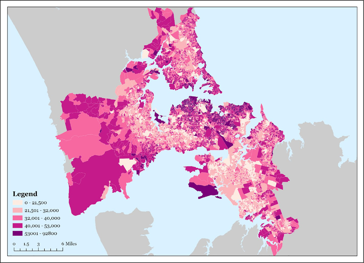
Median income (2018) by SA1, Auckland.

Source: Authors with Auckland Council (2022) Geomap and New Zealand Census (2018).

Figure B2.

Median housing value (2021) by SA1, Auckland.

Source: Authors with Auckland Council (2022) and Relab° (2022).

References

- Asquith A, McNeill J and Stockley E (2021a) Amalgamation and Auckland City: A New Zealand success story? Australian Journal of Public Administration 80(4): 977–986. [Google Scholar]
- Asquith B, Mast E and Reed D (2021b) Local effects of large new apartment buildings in low-income areas. The Review of Economics and Statistics 105(2): 359–375. [Google Scholar]
- Atkinson-Palombo C (2010) Comparing the capitalisation benefits of light-rail transit and overlay zoning for single-family houses and condos by neighborhood type in metropolitan Phoenix, Arizona. Urban Studies 47(11): 2409–2426. [DOI] [PubMed] [Google Scholar]
- Auckland Council (2013) The proposed Auckland Unitary Plan, notified 30 September 2013. Auckland Council, Government of New Zealand. Available at: https://unitaryplan.aucklandcouncil.govt.nz/Pages/Plan/Book.aspx?exhibit=ProposedAucklandUnitaryPlan&hid=89389 (accessed 21 August 2022). [Google Scholar]
- Auckland Council (2017) National policy statement on urban development capacity 2016: Housing, business development Auckland. Auckland Council, Government of New Zealand. Available at: https://knowledgeauckland.org.nz/publications/national-policy-statement-on-urban-development-capacity-2016-housing-and-business-development-capacity-assessment-for-auckland/ (accessed 10 June 2022). [Google Scholar]
- Auckland Council (2019) A brief history of Auckland’s urban form. Auckland Council, New Zealand Government. Available at: https://knowledgeauckland.org.nz/media/1419/a-brief-history-of-aucklands-urban-form-2019-web.pdf (accessed 14 July 2022). [Google Scholar]
- Auckland Council (2021a) Auckland Unitary Plan Operative in part 15 November 2016. Auckland Council, Government of New Zealand. Available at: https://unitaryplan.aucklandcouncil.govt.nz (accessed 10 June 2022). [Google Scholar]
- Auckland Council (2021b) General property revaluation. Available at: https://www.auckland-council.govt.nz/property-ratesvaluations/our-valuation-of-your-property/Pages/l-property-rev.aspx (accessed 8 February 2022).
- Auckland Council (2022) Geomap. Available at: https://unitaryplanmaps.aucklandcouncil.govt.nz/upviewer/ (accessed 24 April 2023).
- Auckland Council (n.d.) Schedule 15: Special character schedule statements and maps [PDF file]. Available at: https://unitaryplan.aucklandcouncil.govt.nz/Images/Auckland%20Unitary%20Plan%20Operative/Chapter%20L%20Schedules/Schedule%2015%20Special%20Character%20Schedule%20Statements%20and%20Maps.pdf (accessed 28 April 2023).
- Been V and McDonnell S (2010) How Have Recent Rezonings Affected the City’s Ability to Grow? Policy Brief. New York, NY: NYU Furman Center, Wagner School of Public Service. [Google Scholar]
- Bond EW and Coulson NE (1989) Externalities, filtering, and neighborhood change. Journal of Urban Economics 26(2): 231–249. [Google Scholar]
- Bratu C, Harjunen O and Saarimaa T (2023) City-wide effects of new housing supply: Evidence from moving chains. Journal of Urban Economics 133: 103528. [Google Scholar]
- Brueckner J (1977) The determinants of residential succession. Journal of Urban Economics 4(1): 45–59. [Google Scholar]
- Brueckner JK (1980) Residential succession and land-use dynamics in a vintage model of urban housing. Regional Science and Urban Economics 10(2): 225–240. [Google Scholar]
- Cheung KS, Wong SK, Wu H, et al. (2021) The land governance cost on co-ownership: A study of the cross-lease in New Zealand. Land Use Policy 108: 105561. [Google Scholar]
- Cheung KS, Yiu CY and Guan Y (2022) Homebuyer purchase decisions: Are they anchoring to appraisal values or market prices? Journal of Risk and Financial Management 15(4): 159. [Google Scholar]
- Clapp JM, Salavei BK and Wong SK (2012) Empirical estimation of the option premium for residential redevelopment. Regional Science and Urban Economics 42(1): 240–256. [Google Scholar]
- Corlett E and Cassidy C (2021) New Zealand has adopted a radical rezoning plan to cut house prices – could it work in Australia? The Guardian, 15 December. Available at: https://www.theguardian.com/world/2021/dec/15/new-zealand-has-adopted-a-radical-rezoning-plan-to-cut-house-prices-could-it-work-in-australia (accessed 14 July 2022).
- Coughlan T (2022) Auckland Council villa protections may break law – Government. New Zealand Herald, 4 September. Available at: https://www.nzherald.co.nz/nz/politics/auckland-council-villa-protections-may-break-law-government/53PK4VCO3PI2TJXZIYYOCVLTQI/ (accessed 24 April 2023).
- Denoon-Stevens SP and Nel V (2020) Towards an understanding of proactive upzoning globally and in South Africa. Land Use Policy 97:104708 [Google Scholar]
- Dong H (2021) Exploring the impacts of zoning and upzoning on housing development: A quasi-experimental analysis at the parcel level. Journal of Planning Education and Research. Epub ahead of print 1 February 2021. DOI: 10.1177/0739456X21990728. [DOI] [Google Scholar]
- Donnell H (2021) An anti-housing Trojan horse. Greater Auckland, 24 November. Available at: https://www.greaterauckland.org.nz/2021/11/24/an-anti-housing-trojan-horse/ (accessed 24 April 2023).
- Dougherty C (2020) Golden Gates: The Housing Crisis and a Reckoning for the American Dream. New York, NY: Penguin Random House. [Google Scholar]
- Dougherty C (2021) After years of failure, California lawmakers pave the way for more housing. The New York Times, 26 August. Available at: https://www.nytimes.com/2021/08/26/business/california-duplex-senate-bill-9.html (accessed 24 April 2023).
- Einstein K, Glick D and Palmer M (2019) Neighborhood Defenders: Participatory Politics and America’s Housing Crisis. Cambridge: Cambridge University Press. [Google Scholar]
- Fox J (2022) What happened when Minneapolis ended single-family zoning. Bloomberg, 20 August. Available at: https://www.bloomberg.com/opinion/articles/2022-08-20/what-happened-when-minneapolis-ended-single-family-zoning (accessed 24 April 2023).
- Freeman L and Schuetz J (2017) Producing affordable housing in rising markets: What works? Cityscape: A Journal of Policy Development and Research 19(1): 217–236. [Google Scholar]
- Freemark Y (2019) Housing arguments over SB 50 distort my upzoning study. Here’s how to get zoning changes right. The Frisc, 22 May. Available at: https://thefrisc.com/housing-arguments-over-sb-50-distort-my-upzoning-study-heres-how-to-get-zoning-changes-right-40daf85b74dc (accessed 24 April 2023). [Google Scholar]
- Freemark Y (2020) Upzoning Chicago: Impacts of a zoning reform on property values and housing construction. Urban Affairs Review 56(3): 758–789. [Google Scholar]
- Gabbe CJ (2018) Why are regulations changed? A parcel analysis of upzoning in Los Angeles. Journal of Planning Education and Research 38(3): 289–300. [Google Scholar]
- Gabbe CJ (2019) Changing residential land use regulations to address high housing prices: Evidence from Los Angeles. Journal of the American Planning Association 85(2): 152–168. [Google Scholar]
- Glaeser EL and Gyourko J (2017) The economic implications of housing supply. Journal of Economic Perspectives 31(1): 3–30.29465214 [Google Scholar]
- Greater Auckland (2022) Building consents in July-22. Available at: https://www.greater-auckland.org.nz/2022/09/05/building-consents-in-july-22/ (accessed 24 April 2023).
- Greenaway-McGrevy R and Phillips PCB (2021) The impact of upzoning on housing construction in Auckland. Working Paper No. 009, Centre for Applied Research in Economics. Available at: https://cdn.auckland.ac.nz/assets/business/about/our-research/research-institutes-and-centres/CARE/The%20Impact%20of%20Upzoning%20on%20Housing%20Construction%20in%20Auckland.pdf (accessed 24 April 2023). [Google Scholar]
- Greenaway-McGrevy R, Pacheco G and Sorensen K (2021) The effect of upzoning on house prices and redevelopment premiums in Auckland, New Zealand. Urban Studies 58(5): 959–976. [Google Scholar]
- Hirt S (2013) Form follows function? How America zones. Planning Practice & Research 28(2): 204–230. [Google Scholar]
- Hochberg S (2019) Defining sensitive communities under SB 50. Report, UC Berkeley Terner Center for Housing Innovation, University of California, Berkeley, United States. Available at: https://escholarship.org/uc/item/83r4h4r3 (accessed 24 April 2023). [Google Scholar]
- Jabareen YR (2006) Sustainable urban forms: Their typologies, models, and concepts. Journal of Planning Education and Research 26(1): 38–52. [Google Scholar]
- Kok N, Monkkonen P and Quigley JM (2014) Land use regulations and the value of land and housing: An intra-metropolitan analysis. Journal of Urban Economics 81(3): 136–148. [Google Scholar]
- Kuhlmann D (2021) Upzoning and single-family housing prices: A (very) early analysis of the Minneapolis 2040 plan. Journal of the American Planning Association 87(3): 383–395. [Google Scholar]
- Land Information New Zealand (2011) Rating revaluations handbook – LINZG30700. New Zealand Government. Available at: https://www.linz.govt.nz/resources/regulatory/rating-revaluations-handbook-linzg30700 (accessed 14 July 2022).
- Li X (2021) Do new housing units in your backyard raise your rents? Journal of Economic Geography 22(6): 1309–1352. [Google Scholar]
- Liu L, McManus D and Yannopoulos E (2022) Geographic and temporal variation in housing filtering rates. Regional Science and Urban Economics 93: 103758. [Google Scholar]
- Manville M, Monkkonen P and Lens M (2020) It’s time to end single-family zoning. Journal of the American Planning Association 80(1): 106–112. [Google Scholar]
- Mast E (2019) The effect of new market-rate housing construction on the low-income housing market. Upjohn Institute Working Paper 19–307. Kalamazoo, MI: WE Upjohn Institute for Employment Research. [Google Scholar]
- Monkkonen P (2016) Understanding and challenging opposition to housing construction in California’s urban areas. UCCS White Paper, University of California Center Sacramento, USA. [Google Scholar]
- Monkkonen P (2019) The elephant in the zoning code: Single family zoning in the housing supply discussion. Housing Policy Debate 29(1): 41–43. [Google Scholar]
- Monkkonen P, Carlton I and Macfarlane K (2020a) One to four: The market potential of fourplexes in California’s single-family neighborhoods. UCLA Lewis Center for Regional Policy Studies Working Paper Series, UCLA Lewis Center for Regional Policy Studies, USA. [Google Scholar]
- Monkkonen P, Manville M and Lens M (2020b) Built-out cities? How California cities restrict housing production through prohibition and process. UC Berkeley Terner Center Land Use Working Paper Series. SSRN. Available at: https://ssrn.com/abstract=3630447 (accessed 24 April 2023). [Google Scholar]
- New Zealand Government (n.d.) Census, StatsNZ. Available at: https://www.stats.govt.nz/topics/census (accessed 24 April 2023).
- Pennington K (2021) Does building new housing cause displacement? The supply and demand effects of construction in San Francisco. Working Paper, SSRN. Available at: https://ssrn.com/abstract=3867764 (accessed 24 April 2023). [Google Scholar]
- Phillips RS (1981) A note on the determinants of residential succession. Journal of Urban Economics 9(1): 49–55. [Google Scholar]
- Phillips S (2022) Building up the “zoning buffer”: Using broad upzones to increase housing capacity without increasing land values. UCLA Lewis Center for Regional Policy Studies. Available at: https://www.lewis.ucla.edu/research/building-up-the-zoning-buffer-using-broad-upzones-to-increase-housing-capacity-without-increasing-land-values/ (accessed 24 April 2023).
- Phillips S, Manville M and Lens M (2021) The effect of market-rate development on neighborhood rents. Research Roundup, UCLA Lewis Center for Regional Policy Studies. Available at: https://escholarship.org/uc/item/5d00z61m (accessed 24 April 2023). [Google Scholar]
- Relab (2022) Smarter property data. New Zealand. Available at: https://relab.co.nz/ (accessed 24 April 2023). [Google Scholar]
- Rodrıģuez-Pose A and Storper M (2020) Housing, urban growth and inequalities: The limits to deregulation and upzoning in reducing economic and spatial inequality. Urban Studies 57(2): 223–248. [Google Scholar]
- Rosenthal SS (2014) Are private markets and filtering a viable source of low-income housing? Estimates from a “repeat income” model. American Economic Review 104(2): 687–706. [Google Scholar]
- Saiz A (2010) The geographic determinants of housing supply. Quarterly Journal of Economics 125: 1253–1296. [Google Scholar]
- Schill MH (2005) Regulations and housing development: What we know. Cityscape: A Journal of Policy Development and Research 8(1): 5–20. [Google Scholar]
- StatsNZ (2021) Statistical Area 1 2021 (generalised). Available at: https://datafinder.stats.govt.nz/layer/105162-statistical-area-1-2021-generalised/ (accessed 24 April 2023). [Google Scholar]
- Sweeney JL (1974) A commodity hierarchy model of the rental housing market. Journal of Urban Economics 1(3): 288–323. [Google Scholar]