

Abstract
We propose a novel latent-class approach to detect and account for population stratification in a case-control study of association between a candidate gene and a disease. In our approach, population substructure is detected and accounted for using data on additional loci that are in linkage equilibrium within subpopulations but have alleles that vary in frequency between subpopulations. We have tested our approach using simulated data based on allele frequencies in 12 short tandem repeat (STR) loci in four populations in Argentina.
Introduction
Although the case-control study is one of the primary tools of epidemiology, it has fallen out of favor in studies of the association of a candidate gene with occurrence of disease, because of the possible effect of population stratification (Li 1972; Lander and Schork 1994; Ewens and Spielman 1995). Population stratification occurs when the population under study is assumed to be homogeneous with respect to allele frequencies but in fact comprises subpopulations that have different allele frequencies for the candidate gene. If these subpopulations also have different risks of disease, then subpopulation membership is a confounder (Kleinbaum et al. 1982), and an association between the candidate gene and disease may be incorrectly estimated without properly accounting for population structure.
Unfortunately, the relevant population structure may not be known. Epidemiologic studies may measure crude indicators of subpopulation membership such as race, but the relevant subpopulations may, in fact, be more finely stratified. As a result, genetic epidemiologists have developed methods based on case-parent triads and using the transmission/disequilibrium test (TDT) to measure the association between a candidate gene and disease status (Self et al. 1991; Spielman et al. 1993). However, these approaches require genotyping both of case patients and of their parents (resulting in both an increase in required sequencing and the requirement that at least one parent is available). Worse, some case-parent triads are not informative. Although alternative approaches exist using other relatives (Spielman and Ewens 1998) or a single parent (Sun et al. 1999), all such approaches require some additional ascertainment of relatives and some additional genotyping. Finally, it should be recognized that effects of population stratification may be reintroduced into TDT-related methods that allow for missing parental data. In particular, the assumption that the distribution of genotypes of the sampled parents can be used to make inferences about the missing parents is analogous to the assumption that gene frequencies among case patients can be compared with those among control patients.
Recently, however, several factors have led to a resurgence of interest in case-control studies of gene-disease association (Risch and Merikangas 1996; Morton and Collins 1998; Risch and Teng 1998). Researchers have begun collecting specimens, for genetic analysis in large epidemiologic studies and surveys (National Center for Health Statistics 1994; Surguchov et al. 1996; Daly et al. 2000), that can be used to study a variety of gene-disease and gene-environment associations. Many case-control studies can be conducted using the same stored specimens, without requiring genotypes of relatives of case subjects. Although Wacholder et al. (2000) argue that population stratification of an extent large enough to distort results is unlikely to occur in many realistic situations, it is still important to develop methods that allow for control of population stratification when analyzing case-control studies.
Fortunately, if population substructure affects allele frequencies of the candidate gene, then it should also affect allele frequencies of other genes as well (Devlin and Roeder 1999; Pritchard and Rosenberg 1999). Markers—that is, genes that are markers of population substructure and that (1) segregate independently both from each other and from the candidate gene and (2) are not themselves associated with disease or in linkage disequilibrium with genes associated with disease—can be used to make inferences about the existence of population substructure in a sample (Pritchard and Rosenberg 1999) and even to reconstruct the underlying population substructure in an observed sample (Pritchard et al. 2000a). Additionally, binary markers (e.g., single-nucleotide polymorphisms) can be used to control for differences in relatedness between cases and controls that occur when population substructure confounds the relation between disease and a candidate gene (Devlin and Roeder 1999; Bacanu 2000; Devlin, in press).
In this study, we use a novel latent-class analysis to use data on markers to make inferences about the association between a candidate gene and the occurrence of disease in a population that may be subject to population stratification. Latent-class methods have been used extensively in sociology to analyze questionnaire data by using correlations in responses to related questions to make inferences about subgroups of people with common attitudes or beliefs (see, e.g., Henry 1983). Inferences concerning population substructure in a single sample, using correlations in genotypes at loci that are unrelated to disease, can also be accomplished using latent-class analysis. However, a case-control study comprises two separate samples (one of case subjects and the other of control subjects); if different subpopulations have different disease risks, we can expect the proportions of case patients from each subpopulation (class probabilities) to differ from the corresponding proportions of control subjects. Two separate latent-class analyses, one using data from case subjects and the other using data from control subjects, can lead to logical inconsistency, because different population substructure might be inferred in each population. If this occurs, data from case subjects and control subjects could not be recombined to calculate the odds ratio for the association between the candidate gene and disease. The approach we take here properly accounts for the differences between the sample of case subjects and the sample of control subjects, while assuming that case subjects and control subjects derive from the same target population.
Model
The quantities of primary interest are those that relate disease (denoted by the binary variable D) to a (possibly vector-valued) genetic risk factor G. This relation may be confounded by the existence of population stratification. Unfortunately, we may not know which subpopulations have the differential rates of disease or prevalence of the candidate gene G that, if not properly accounted for, will result in improper inference about the relation between D and G. In addition, separate sampling of cases and controls must be properly accounted for in any analysis.
As a heuristic approximation of the complex genetic history that may have led to the current population substructure, we assume that the overall population comprises K subpopulations, each having different frequencies of G and D. In the development below, we suppress an index i corresponding to the ith individual. We denote by Z the (unmeasured) covariable Z that indicates the subpopulation to which an individual belongs. Because different subpopulations may have different frequencies of other mutually independent marker genes that are unrelated to disease, we propose to use a novel latent-class approach to infer the population substructure while simultaneously estimating parameters relating G to D. Let Xcℓ denote the allele at marker ℓ on chromosome c=1, 2 (numbering of chromosomes is arbitrary) and let X=(X11, X21,⋅⋅⋅, X2L), where L is the number of marker loci. In the analysis that follows, we assume that Hardy-Weinberg equilibrium holds in each subpopulation. Relaxing this assumption by considering Xℓ to represent genotype data is possible; however, human populations rarely show much divergence from Hardy-Weinberg equilibrium once population substructure has been accounted for (Committee on DNA Forensic Science 1996, pp. 104 and references cited therein).
We assume that the genes at the marker loci are unrelated to disease, that is,
We further assume that, for persons in the same subpopulation, the marker loci are in linkage equilibrium with the candidate gene G, so that
This assumption can be met, for example, by choosing marker loci on different chromosomes from the chromosome where G is found. Finally, we assume that Z is a confounder but not an effect modifier—that is, that
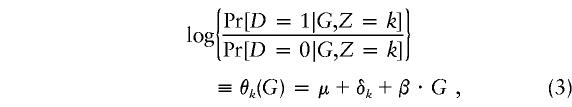 |
where we take  for identifiability. In a case-control study, we cannot usually expect to estimate μ, although we will see that the δks are, in fact, estimable and that there is even some information on μ. An immediate consequence of equations (1) and (2) is that Pr[X|G,Z,D]=Pr[X|Z]. We assume Hardy-Weinberg equilibrium holds within each stratum, so that
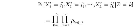 |
where pℓkj=Pr[Xcℓ=j|Z=k] is the proportion of persons in subpopulation k having allele j at marker locus ℓ.
Because case subjects and control subjects can be considered as representative samples from the segments of the population with and without disease, we base our inference on Pr[X,G|D]. To account for population stratification, we write
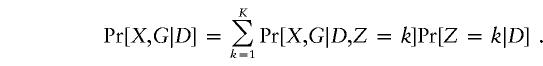 |
Assume that G takes M+1 values g0≡0,⋅⋅⋅,gM; let πdk=Pr[Z=k|D=d] be the proportions of persons in each subpopulation by disease status; let γkm= Log{Pr[G=gm|D=0,Z=k]/Pr[G=g0|D=0,Z=k]}; and let γk=(γk1,⋅⋅⋅,γkM). After some algebra, we find that
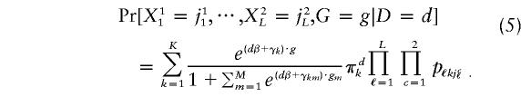 |
Likelihood (5) is for a single individual; the likelihood for all individuals in the study is the product of terms such as (5) for each participant.
We may choose β, π0k, and π1k as separate parameters to be maximized; it is possible to show that choosing π0k and π1k as independent parameters is equivalent to a model in which we choose π0k and δk as parameters. The situation is more complicated with parameters γkm. For example, if G has r alleles, then there are r(r+1)/2-1 values of γkm for each k. However, if Hardy-Weinberg equilibrium holds in each subpopulation, then only r-1 parameters are required to specify all the γkms for a given k. Unfortunately, even if Hardy-Weinberg equilibrium holds in each subpopulation, it will not hold among control subjects if the candidate gene is, in fact, associated with disease (Sasieni 1997). This is because the distribution of G among control subjects is given by
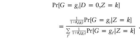 |
Hence, the overall magnitude of the departures from Hardy-Weinberg equilibrium among control subjects is primarily determined by μ, as defined in equation (3). If we assume a rare disease (corresponding to μ being large and negative), then Pr[G=gj|D=0,Z=k]≈Pr[G=gj|Z=k], and we can maximize (5) directly with respect to parameters β, π0k, π1k and parameters in the model for Pr[G=gj|Z=k]. Even if the disease is rare, the distribution of G among case subjects does not correspond to Hardy-Weinberg equilibrium unless β=0.
In the absence of an approximation of rare disease, we can still proceed without difficulties, as long as G is binary (i.e., if certain genotypes correspond to low risk and others to high risk). In this case, there is a single γk for each k, which may be treated as an independent parameter in place of Pr[G=1|Z=k]. We feel that it is unlikely that a reasonable estimate of μ can be obtained using case-control data alone, and, hence, either the approximation of rare disease should be made or several analyses using various binary genotypes G should be undertaken.
Although the likelihood (5) can be evaluated directly, the large number of parameters suggests use of the E-M algorithm. In this approach, the subpopulation to which each individual belongs is treated as missing data. This is easily accomplished, because all calculations in the E step can be carried out in closed form and the values of πdk and pℓkj can be estimated in closed form. To estimate the parameters β and γk, a simple maximization must be carried out, corresponding to fitting the model
 |
to K2×(M+1) tables, using maximum likelihood. In this calculation, the “data” are the expected proportion of persons having D=d, Z=k, and G=g, available from the previous E step. If M=1 (i.e., if G is binary), then the calculation reduces to a logistic regression analysis in which G is considered the outcome and D and Z are explanatory variables. If M>1, then the approximation of rare disease should be made and an appropriate model for γkm should be chosen to reflect Hardy-Weinberg equilibrium among the controls. For example, if M=2 and outcomes G=g0,g1 and g2 correspond to persons having zero, one, or two copies of a disease-causing allele, then we take γk=(ln2+αk,2αk), where αk is the log of the odds that a person in the kth subpopulation has the disease-causing allele.
Likelihood (5) can be maximized using the E-M algorithm for a fixed number of subpopulations K. To estimate the number of subpopulations, we propose to select the value of K that minimizes the Akaike information criterion (AIC), which is given by -2logL+2P, where P is the number of parameters fit. If PG is the number of parameters required to specify γk for a single stratum and Pβ is the number of free parameters in β, then P=K*(PG+ total no. of marker alleles − no. of marker loci) + 2*(K-1)+Pβ. To estimate K, we start with a single population (K=1) and increase K by 1 until the AIC begins to increase. This procedure assumes that the first minimum in the AIC corresponds to the global minimum. In some small-scale simulations, this appears to be the case (results not shown). Moreover, when the number of subpopulations K is greater than or equal to the number used to generate the data, the values of β appear to change very little (results not shown). Additional details on the E-M algorithm used are found in the Appendix.
Because of the large number of parameters fit, we recommend that variance estimates be calculated using a parametric bootstrap procedure (Efron and Tibshirani 1998), conditional on the total numbers of case subjects and control subjects. In this procedure, simulated data sets are constructed using the parameter estimates obtained from fitting the latent-class model. Specifically, for each observation data on subpopulation is generated conditional on case or control status using the estimated values of π1k, for case subjects, or of π0k, for control subjects. Then, data on the candidate gene is simulated using (6) and the estimated values of β and the appropriate γk. Finally, marker values are simulated using the estimated values of pℓkj. A total of T such data sets are generated, and estimates of β, denoted by  , are obtained. The variance of
  can then be estimated to be the empirical variance of the
  values, and confidence intervals can be calculated using the percentiles of the
  values (Efron and Tibshirani 1998).
Example 1: Discrete Subpopulations
A classic example of population substructure affecting a case-control study occurred in a population that was an admixture of European and Pima ancestry (Knowler et al. 1988). In this study, an association between a candidate gene and insulin-dependent diabetes type 1 actually resulted from confounding caused by population substructure. To illustrate our approach, we considered an analogous scenario based on an admixture of Europeans and American Indians. Sala et al. (1998, 1999) have published allele frequency data on twelve short tandem repeat (STR) loci in Argentineans of European ancestry, as well as in three Argentinean American Indian groups (Mapuche, Tehuelche, and Wichi). We have used these allele frequencies to simulate a population that comprises four subpopulations that differ in disease risk and frequency of a candidate-gene allele that is associated with disease.
Because Sala et al. (1998, 1999) sampled ∼10 times more persons of European ancestry than persons of any of the other three ethnic groups, we combined some STR alleles to reduce the number of alleles having zero frequency in one or more American Indian populations. As a general rule, we combined adjacent alleles until the allele frequency in at least one population was ⩾5%. The resulting allele frequencies are shown in table 1. An exception was HPRTB, where allele frequencies of zero were allowed for small numbers of repeats in the American Indian groups, since there appears to be a consistent increase in number of repeats in the non-European groups. Occurrence of alleles in one population that are missing in another makes identification of population substructure easier; hence, our decision to combine alleles actually makes it more difficult to identify subpopulations. All STR loci but HPRTB are autosomal; to avoid generating gender, we used the HPRTB allele frequencies to generate data as if HPRTB were an autosomal locus.
Table 1.
Allele Frequencies for 12 STR Loci in Four Argentinean Populationsa
|
Population |
||||
| STRLocus | European | Mapuche | Tehuelche | Wichi |
| FABP | .589 | .683 | .732 | .485 |
| .110 | .058 | .107 | .162 | |
| .300 | .260 | .161 | .353 | |
| CSF1P0 | .330 | .266 | .339 | .226 |
| .313 | .282 | .232 | .194 | |
| .298 | .367 | .411 | .581 | |
| .059 | .085 | .018 | .000 | |
| D6S366 | .082 | .091 | .143 | .000 |
| .204 | .114 | .071 | .000 | |
| .277 | .341 | .446 | .557 | |
| .119 | .136 | .036 | .086 | |
| .091 | .125 | .036 | .029 | |
| .183 | .159 | .143 | .200 | |
| .028 | .011 | .018 | .071 | |
| .015 | .023 | .107 | .057 | |
| F13A | .151 | .222 | .357 | .173 |
| .060 | .122 | .125 | .077 | |
| .202 | .122 | .054 | .346 | |
| .209 | .178 | .143 | .115 | |
| .325 | .344 | .304 | .288 | |
| .053 | .111 | .017 | .000 | |
| FES | .260 | .170 | .143 | .257 |
| .420 | .500 | .714 | .543 | |
| .247 | .284 | .107 | .043 | |
| .073 | .045 | .036 | .157 | |
| TH01 | .233 | .526 | .286 | .132 |
| .250 | .298 | .429 | .721 | |
| .105 | .088 | .018 | .000 | |
| .185 | .026 | .089 | .015 | |
| .226 | .140 | .179 | .132 | |
| HPRTB | .032 | .000 | .000 | .000 |
| .179 | .032 | .091 | .000 | |
| .317 | .323 | .227 | .357 | |
| .285 | .403 | .591 | .167 | |
| .137 | .242 | .091 | .357 | |
| .050 | .000 | .000 | .119 | |
| vWA | .063 | .096 | .036 | .014 |
| .099 | .077 | .054 | .014 | |
| .294 | .577 | .429 | .514 | |
| .297 | .125 | .214 | .343 | |
| .246 | .212 | .268 | .114 | |
| D13S317 | .09 | .02 | .000 | .000 |
| .16 | .24 | .150 | .464 | |
| .06 | .07 | .050 | .179 | |
| .29 | .12 | .150 | .089 | |
| .25 | .26 | .300 | .089 | |
| .10 | .18 | .225 | .179 | |
| .04 | .11 | .125 | .000 | |
| D7S820 | .156 | .07 | .05 | .0 |
| .115 | .05 | .05 | .07 | |
| .276 | .22 | .175 | .125 | |
| .245 | .42 | .525 | .45 | |
| .159 | .21 | .20 | .25 | |
| .046 | .03 | .0 | .105 | |
| D16S539 | .156 | .11 | .225 | .125 |
| .100 | .13 | .075 | .232 | |
| .294 | .24 | .10 | .321 | |
| .159 | .37 | .55 | .250 | |
| .195 | .15 | .05 | .071 | |
| RENA-4 | .772 | .719 | .881 | .69 |
| .074 | .229 | .023 | .0 | |
| .153 | .041 | .095 | .31 | |
We generated 500 data sets using the allele frequencies in table 1, assuming that Argentinean Europeans constituted 70% of a hypothetical target population and that each American Indian group constituted 10%. In addition, data on a biallelic candidate gene was generated, which was assumed to be in Hardy-Weinberg equilibrium in each subpopulation. Persons who were homozygous for the disease-causing allele had an increased risk of disease corresponding to a log-odds ratio of 1.0 (relative risk =2.72). Persons who were heterozygous for the disease-causing allele had no increase in risk. The prevalence of the disease-causing allele was chosen to be 0.277, 0.341, 0.446, and 0.557 in the European, Mapuche, Tehuelche, and Wichi populations, respectively (the frequencies of allele 3 of locus D6S366). The log of the odds of disease among persons with zero or one copies of the disease-causing allele was −5, −4, −3, and −3 in the European, Mapuche, Tehuelche, and Wichi populations, respectively. These values correspond to a prevalence of disease among persons without the disease-causing allele of 0.7%, 1.8%, 4.7%, and 4.7%, respectively. Data were generated until 125 case patients and 125 control patients were obtained. Because the disease is rare, the distribution of ethnic groups among control patients was approximately that of the target population (70.5%, 10.1%, 9.6%, and 9.8% in the 500 simulated data sets). However, the distribution of ethnic groups in the case patients was noticeably different, with 26.1% European, 10.7% Mapuche, 29.8% Tehuelche, and 33.4% Wichi.
In tables 2 and 3, we show the results of a number of analyses of these simulated data. The crude analysis corresponds to calculation of the association between disease and the candidate gene using a single 2×3 table. The second analysis is the latent-class analysis that estimates β1 and β2 simultaneously, assuming the disease is rare. The third and fourth analyses are the latent-class binary genotype model estimates of β1 (using data only from persons with zero or one copy of the disease-causing allele) and β2 (using data only from persons with zero or two copies of the disease-causing allele). Finally, we give results of two analyses that use the true subpopulation data, in which β is estimated by maximization of the likelihood for marker and candidate-gene data, given case/control status and knowledge of subpopulation. The first makes the rare-disease approximation (i.e., assumes Hardy-Weinberg equilibrium in control patients) and estimates β1 and β2 simultaneously. The second estimates β1 (using data only from persons with zero or one copies of the disease-causing allele) and β2 (using data only from persons with zero or two copies of the disease-causing allele) using only binary candidate-allele data. For all simulations, the average and empirical standard error of parameter estimates from the 500 simulations are presented.
Table 2.
Results of Analyses of Simulated Data Using 12 STR Loci with 250 Study Participants (125 Case Patients and 125 Control Patients) and Four Distinct Subpopulations
|
Parameter |
|||
| Analysisand Variable | β1 | β2 | K |
| True value | .000 | 1.000 | 4.00 |
| Crude analysis: | |||
| Average | .366 | 1.760 | 1.00 |
| Standard error | .285 | .370 | … |
| Latent class: | |||
| Rare disease: | |||
| Average | .061 | 1.006 | 3.53 |
| Standard error | .293 | .453 | .76 |
| Binary genotype: | |||
| Average | .021 | 1.095 | 3.14, 3.27 |
| Standard error | .377 | .540 | .91, .62 |
| Full data: | |||
| Rare disease: | |||
| Average | .052 | .995 | 4.00 |
| Standard error | .276 | .405 | … |
| Binary genotype: | |||
| Average | −.002 | 1.043 | 4.00 |
| Standard error | .331 | .470 | … |
Table 3.
Results of Latent-Class Analyses of Simulated Rare-Disease Data Using Six STR Loci with Varying Sample Sizes and Four Distinct Subpopulations
|
Parameter |
|||
| Sample Size(Cases/Controls)and Variable | β1 | β2 | K |
| True value | .000 | 1.000 | 4.00 |
| 125/125: | |||
| Average | .023 | .883 | 3.32 |
| Standard error | .865 | 1.718 | .69 |
| 250/250: | |||
| Average | .023 | .962 | 3.37 |
| Standard error | .226 | .394 | .61 |
Because β1 and β2 from the crude analysis differ markedly from the values used to generate the data (β1=0 and β2=1), the population substructure has a large effect. However, the results of the latent-class analysis are close to the true values, even though we used only 12 STR loci to reconstruct the population substructure. In addition, the standard errors of the rare-disease latent-class estimators are only slightly higher than that of the maximum-likelihood estimator obtained using information on true subpopulation membership (e.g., 0.453 for the latent-class rare-disease estimate of β2, compared with 0.405 for the equivalent analysis using the true population substructure). This indicates that group membership is determined with fairly high precision. The standard error for the binary-genotype analyses is higher than the rare-disease approximation, because each analysis uses fewer data than the rare-disease model does. Given the estimate of β1≈0 from either the rare-disease analysis or the binary-genotype analysis using only persons with zero or one copy of the disease allele, another valid analysis would be a comparison of persons with zero or one copy of the disease allele with persons with two copies in a binary-genotype analysis.
To examine the effect of the number of STR loci on our estimator, we also analyzed the simulation data sets using only the first six STR loci in table 1, by means of the rare-disease model (table 3). The estimator of β1 is still good, but β2 is noticeably further from its true value. However, even with only six STR loci, adequate performance can be achieved by increasing the sample size to 500 (250 case patients and 250 control patients).
The estimated number of subpopulations,  , was chosen to minimize the AIC, as was described in section 2. The value of
  obtained by our method was, on average, lower than the true value of 4, possibly because one subpopulation constitutes only 10% of cases and controls. When we increased the sample size to 250 case patients and 250 control patients, the average number of subpopulations detected increased to four (which was also the number of subpopulations most frequently selected).
We assessed the coverage (proportion of intervals containing the true value) of confidence intervals obtained using the parametric bootstrap procedure described in the previous section. For each of 200 data sets (each with 125 case patients, 125 control patients and using all 12 markers), we generated 200 bootstrap replicates and calculated confidence intervals for β1 and β2 using the percentile method (Efron and Tibshirani 1998). Figures 1 and 2 compare the nominal and actual coverage of these confidence intervals. Ideal behavior corresponds to a 45° line corresponding to nominal and actual coverage being equal. The 95% confidence interval for β1 contained the true value of 0 in 98% of the simulations, and the 95% confidence interval for β2 contained the true value 1.0 in 97% of the simulations. Ideally, >200 bootstrap replicates should be used to calculate a confidence interval, and we chose only 200 replicates per data set, to reduce the computational burden of analyzing 200 data sets. In practice, at least 500 replicates should be used. The bootstrap can also be used to estimate the standard error of  . The average bootstrap estimators of the standard error of
  and
and  for the rare-disease model are 0.313 and 0.498, close to the standard errors of the simulated data sets (0.293 and 0.453, respectively).
Figure 1.

Nominal versus actual coverage of bootstrap confidence intervals for β1 (proportion of 100α% confidence intervals that contain the true value of β1) for the discrete subpopulation data in example 1.
Figure 2.

Nominal versus actual coverage of bootstrap confidence intervals for β2 (proportion of 100α% confidence intervals that contain the true value of β2) for the discrete subpopulation data in example 1.
To assess the performance of our method when stratification was not present, we also generated case-control data as above, but sampled individuals exclusively from the European subpopulation. The results of analyses of 500 simulated data sets using the rare-disease model are summarized in table 4. The method performed well, properly identifying the true number of subpopulations (1) in 74% of the data sets. The average of the estimates of parameters β1 and β2 is also close to their true values, and the variability of these estimates is close to the values obtained by maximum likelihood, using a model that ignores stratification.
Table 4.
Results of Analyses of Simulated Data Using 12 STR Loci with 250 Study Participants (125 Case Patients and 125 Control Patients) and No Population Substructure
|
Parameter |
|||
| Analysisand Variable | β1 | β2 | K |
| True value | .000 | 1.000 | 1.00 |
| Latent class: | |||
| Rare disease: | |||
| Average | .041 | 1.023 | 1.34 |
| Standard error | .253 | .414 | .66 |
| Binary genotype: | |||
| Average | .012 | 1.086 | 1.30, 1.25 |
| Standard error | .276 | .463 | .64, .60 |
| Full data: | |||
| Rare disease: | |||
| Average | .028 | 1.017 | 1.00 |
| Standard error | .229 | .392 | … |
| Binary genotype: | |||
| Average | .013 | 1.076 | 1.00 |
| Standard error | .267 | .448 | … |
Example 2: Continuous Admixture of Ancestral Populations
The latent-class model we have described assumes the existence of discrete subpopulations, each with a set of characteristic allele frequencies. Although this model may accurately describe some populations, a more common situation may be many small, related subpopulations or a continuous mixture of ancestral populations. However, even if the underlying population is a continuous mixture, the discrete-subpopulation model may provide adequate inference on the odds ratio relating the candidate gene and disease. It is known that a stratified analysis with a few well-chosen strata often can control for confounding, even if the confounding is caused by continuous variables (Rosenbaum and Rubin 1984). To assess this, we conducted a simulation study in which data were generated using a continuous mixture model (corresponding to an infinite number of subpopulations). Specifically, we assumed that the population was a continuous admixture of four ancestral populations. We assumed the four Argentinean populations described in example 1 were the ancestral populations. Following Pritchard et al. (2000a), for each individual we generated a Dirichlet random variable Y with four components y1,⋅⋅⋅,y4. The kth component of Y represents the probability that an allele for this individual is from ancestral population k. As a result, the frequency of allele j at locus ℓ for an individual with random variable Y can be written as y1pℓ1j+⋅⋅⋅+y4pℓ4j, where, in a slight abuse of notation, pℓkj denotes the frequency of allele j at locus ℓ in the kth ancestral population. The parameters of the Dirichlet distribution used were (0.7, 0.1, 0.1, 0.1), so that 70% of the total genome of the target population was of European origin, with a contribution of 10% from each of the American Indian populations. This choice of parameters ensures a wide range of variability among individuals, and ∼40% of persons had a plurality of their genome taken from one of the American Indian populations. We also assumed the risk of disease was a linear function of Y. Letting ν=(-5.0, -4.0, -3.0, -3.0), we took the odds of disease for a person with Dirichlet vector y to be ν·y. Hence, the prevalence of disease among persons without the disease-causing allele ranged from 0.7%, for persons with entirely European ancestry, to 4.7%, for persons with exclusively Tehuelche or Wichi ancestry. Among cases, the proportions of persons with European, Mapuche, Tehuelche, and Wichi as the most prevalent ancestral component were 46%, 10%, 21%, and 23%, respectively, whereas the equivalent proportions among controls were 60%, 9%, 15%, and 16%.
The results of fitting the latent-class model to these data are shown in table 5. Generally the mean value of the estimates of β1 and β2 were comparable to the situation in example 1, in which the population was a discrete mixture. On average, three subpopulations were chosen using the AIC criterion. For the relatively small sample size we considered, the bias in the estimated log-odds ratio for the latent-class model was ∼0.08. The ratio of the standard error of the latent-class estimator of β over the standard error of the “full data” estimator of β obtained by maximizing the likelihood of the genotype given disease status and knowledge of the Dirichlet vector Y is larger than the equivalent comparison when the underlying population substructure is discrete. To determine how sample size affects performance of the latent discrete latent-class model with continuous admixture data, we increased the sample size to 500 cases and 500 controls. These results, also shown in table 5, indicate that the bias of the latent-class model decreases considerably when the sample size is increased. The increase in variability of the latent-class estimators over the full-data model is also reduced. Additionally, the estimated number of subpopulations increased. Although we have not considered it, it is reasonable to expect that an increase in the number of informative markers would also improve performance.
Table 5.
Results of Analyses of Simulated Data Using 12 STR Loci with 250 Study Participants (125 Case Patients and 125 Control Patients) and a Continuous Admixture of Four Ancestral Subpopulations
|
Parameter |
|||
| Sample Size(Cases/Controls),Analysis, andVariable | β1 | β2 | K |
| True value | .000 | 1.000 | ∞ |
| 125/125: | |||
| Crude analysis: | |||
| Average | .178 | 1.415 | 1.00 |
| Standard error | .283 | .402 | … |
| Latent class: | |||
| Average | .077 | 1.079 | 3.05 |
| Standard error | .291 | .485 | 1.04 |
| Full data: | |||
| Average | .027 | .992 | ∞ |
| Standard error | .261 | .387 | … |
| 500/500: | |||
| Latent class: | |||
| Average | .044 | 1.018 | 4.40 |
| Standard error | .141 | .224 | 1.41 |
| Full data: | |||
| Average | .021 | .990 | ∞ |
| Standard error | .131 | .193 | … |
Because the number of subpopulations seemed small in light of the large variability of the Dirichlet distribution used to generate the data, it seemed possible that the coverage of confidence intervals calculated using the parametric bootstrap would be too low (recall that, for a given data set, each bootstrap replicate is generated assuming  subpopulations, where
  is the estimated number of subpopulations obtained by minimizing the AIC for that data set). Surprisingly, this apparently was not the case. Coverage of bias-corrected (Efron and Tibshirani 1998) confidence intervals for β1 and β2 for our simulations with 125 cases and 125 controls are shown in figures 3 and 4, respectively. The departure from linearity in figure 4 is not significant (Kolmogorov-Smirnov test, P>.15), indicating failure to reject the hypothesis that the actual coverage is equal to the nominal coverage). The average bootstrap estimators of the standard error of
  and
and  for the rare-disease model are 0.293 and 0.468, close to the standard errors of the simulated data sets (0.291 and 0.485, respectively).
Figure 3.

Nominal versus actual coverage of bootstrap confidence intervals for β1 (proportion of 100α% confidence intervals that contain the true value of β1) for the continuous admixture data in example 2.
Figure 4.

Nominal versus actual coverage of bootstrap confidence intervals for β2 (proportion of 100α% confidence intervals that contain the true value of β2) for the continuous admixture data in example 2.
Hypothesis Testing
We have focused on parameter estimation in this paper. However, several approaches to hypothesis testing are also possible. One approach corresponding to a Wald test is to fit the latent-class model and obtain bootstrap confidence intervals for the odds ratio parameters; the null hypothesis is rejected at the level of 100(1-α)% if the corresponding confidence interval excludes the null value.
An alternative would be a permutation test in which the case or control status was randomly reassigned (in such a way that the total number of cases and controls was preserved). Then, the latent-class model could be fit to the permuted data. A significant association at the level of 100(1-α)% would be found if the odds ratio βk, estimated from the true data, were larger than the corresponding quantile of βk values, estimated using the permuted data.
A final alternative would be to use a likelihood-ratio test, maximizing the likelihood as described above and then again, while holding the odds ratio fixed at its null value. Although this approach is computationally easier, the large number of nuisance parameters (the marker-allele frequencies) makes it somewhat suspect. Additionally, the null and alternative likelihood calculations would have to be constrained to have the same number of subpopulations, which is contrary to the spirit of our approach. Hence, the likelihood-ratio test probably should not be used without further simulation studies of its validity.
Discussion
Differences in allele frequencies between subpopulations result from population genetic processes, including mutation, selection, genetic drift, and population dynamics (e.g., inbreeding or migration). As a result of these processes, a relation may exist between the differences in allele frequency across subpopulations in a candidate gene and differences in allele frequency in STR or other marker genes. If selection does not act on alleles of the candidate gene, then differences in allele frequency in a candidate gene between subpopulations and differences in allele frequency in STR or other marker genes should be comparable. As a consequence, the extent to which confounding can be caused by population substructure should be related to the ease with which it can be detected and accounted for, with larger effects being easier to detect (Pritchard and Rosenberg 1999). The simulation example we considered had a great deal of population stratification and a correspondingly large amount of confounding. We were able to account for the effect of population stratification using only 12 STR loci (even after some pooling of alleles); even our analyses that used only 6 STR loci were successful. Presumably, a population with less stratification would require more marker loci (and, possibly, a larger sample size) to resolve the population structure; however, we would expect that the confounding, caused by population structure, of the association of a candidate gene with disease would be concomitantly smaller. Selection acting on alleles of the candidate gene may alter this relation. If selection reduces differences in allele frequencies of the candidate gene, then population substructure is still identifiable, but confounding is less than otherwise might be expected. If selection increases differences in allele frequency in the candidate gene, then the situation is more serious. However, in this case, the candidate gene is itself an informative marker of population substructure. If the candidate gene is the only gene with allele frequencies that differ between subpopulations, then our approach (and any other based on inferring population substructure using marker genes) will fail. However, this case is unlikely to arise in human populations. By selection pressure, we mean differences in reproductive fitness; the allele frequencies of genes that may be associated with adult-onset cancer, heart disease, or other chronic diseases are unlikely to be altered by selection.
Two general approaches exist to account for population stratification. One is to attempt to model the population substructure; this is the approach we took and is also the approach of Pritchard and colleagues (Pritchard et al. 2000a, 2000b). The other is the genomic control (GC) approach (Devlin and Roeder 1999; Bacanu et al. 2000; Devlin et al., in press). We believe that, within the modeling approach, our approach is superior to that of Pritchard et al. for four reasons. First, our model is a unified treatment of both occurrence of disease and population substructure, whereas that of Pritchard et al. is a two-step approach that estimates substructure first and then tests conditional on the imputed structure. Because our model is unified, we can provide parameter estimates rather than just test hypotheses; the approach of Pritchard et al. cannot be generalized easily to provide parameter estimates. Second, our procedure accounts for the variability in selection of the number of subpopulations, while the test of Pritchard et al. is conditional on the number of subpopulations that are inferred using only the marker data. The bootstrap procedure that we propose for calculation of confidence intervals accounts for variability in the estimated number of subpopulations by estimation of this parameter for each bootstrap replicate. Third, the procedure of Pritchard et al. requires a Gibbs sampler that changes the number of parameters in the model, and this type of sampler is notorious for convergence problems. Our model uses a straightforward likelihood approach. Finally, our model accounts for differences in subpopulation structure that will occur between cases and controls that are ignored by Pritchard et al. who infer substructure without accounting for case and control status. For example, in our simulation, although case patients and control patients were simulated from a population that was 70% European, only 26% of case patients were from the European subpopulation. Because Pritchard et al. test for differences in allele frequencies conditional on population substructure, the candidate gene cannot contribute information about population substructure. In our approach, substructure and disease-gene association are calculated simultaneously; hence, the candidate gene can contribute to inferences about substructure. This is useful because, if population substructure results in confounding, the candidate gene is necessarily informative about population substructure.
Comparison with GC is more difficult, because the GC approach to population stratification is different. In a sense, the GC approach is more general, because it applies to any situation in which cases and controls might have differences in homozygosity (the other major situation being cryptic relatedness, which occurs when case patients may be more likely than control patients to be closely related through a common ancestor). However, the GC approach is limited to binary marker and candidate alleles and requires the additional assumption that the effect of population structure is constant over all loci. Our approach is likelihood-based and, hence, should have better power in situations where a latent-class model correctly describes underlying population substructure. However, an advantage to GC is that an underlying model of the population substructure does not have to be specified. Furthermore, both approaches reduce to the same unstratified analysis when there is no population substructure. It is likely that GC requires more marker loci (although large numbers of biallelic SNP markers should be available soon), whereas continued identification of loci that are highly informative of population substructure (e.g., Dean et al. 1994; Shriver et al. 1997; Parra et al. 1998) should reduce the number of loci required for the latent-class analysis. Finally, GC provides hypothesis tests but not parameter estimates. Because of the differences between GC and our approach, a direct comparison of power, using the example we have considered, is not possible.
Both the approach of Pritchard et al. and GC are tests of association, not methods of estimating association parameters. Estimation of the magnitude of the association between a candidate gene and disease is important, even when population substructure is present. In addition, even though a “significant” amount of population substructure is present, the actual effect on the disease-gene odds ratio can easily be relatively small. Knowing the magnitude of the effect of population stratification on the odds ratio estimate may also be important in assessing the extent of bias in case-control studies in which this stratification may have been ignored.
We used data on 12 STR loci to infer subpopulation membership. These loci were chosen because their use in forensic applications has resulted in publication of allele frequencies in various subpopulations. Forensic applications do not require (and, in fact, are complicated by) varying allele frequencies across subpopulations. Characterization of a set of loci that have maximum variability across human subpopulations to improve identification of the effect of population stratification on case-control studies would be useful. To a great extent, this parallels efforts to find markers that distinguish subpopulations for mapping by admixture linkage disequilibrium or for estimation of ethnic affiliation (Dean et al. 1994; Stephens et al. 1994; Shriver et al. 1997; Parra et al. 1998; Collins et al. 2000). Our initial success and those of Pritchard et al. suggest that persons conducting case-control studies should consider obtaining genotype information from cases and controls at unrelated loci, such as the forensic STR loci we used here to assess and control for the possible effects of population stratification.
Appendix A
Because of the large number of parameters in our latent-class models, it is important to choose good starting values and to take steps to reduce the chance of the program finding a local (rather than global) maximizer of the likelihood. In this appendix, we discuss the algorithm we used to achieve these goals.
We generated starting values for the E-M algorithm as follows: We first identified a family of variables t(r)i, on the basis of a linear score for each allele. Variables t(r)i were chosen using principal components, so that they encompassed as much of the variability as possible in the allele-frequency data. To accomplish this, suppose that allele j at locus ℓ is assigned a numerical score c(r)ℓj and let  , where niℓj is the number of copies of the jth allele at the ℓth locus in the ith study participant. If the values of niℓj are taken to be the ith row of a matrix Y, values of c(r)ℓj correspond to the values of the eigenvector corresponding to the rth largest eigenvalue of the matrix
  , where
  is a centered version of Y.
Let ρ(r)i denote the rank of t(r)i among the study participants. Then, the initial probability that the ith individual was in stratum k was taken to be f(r;0)ik∝e-0.5*(ρi-μk/σ)2 for k=1,⋅⋅⋅,K where μk=n(k-0.5)/K and σ=n(K-0.5)/K. For this choice, note that the  for any r, i, k, and k′.
To avoid excessive influence of the initial value f(r;0)ik, we adopted the following strategy. Let f(m)ik denote the estimate that the ith person is in subpopulation k after m steps of the E-M algorithm. Rather than using f(m)ik to determine new estimates of the parameters β, γ, πdj, and pℓkj, we used  . We used α0=0.5 and selected αm for m⩾1, as follows. If β(m) and γ(m) denote the estimates of β and γ obtained after m steps, then we used αm=αm-1, unless
  , in which case we used αm= 1/2αm-1, where ||x|| denotes the Euclidean norm of the vector x. The algorithm was judged to have converged when δm<10-7, as long as αm<10-7.
For one, two, or three subgroups, our algorithm invariably found the same maximum-likelihood estimates of β, γ, and πdj when the starting values were changed. However, for four or more subgroups, a change in the starting value sometimes resulted in small changes in the final parameter estimates. Hence, whenever the number of subgroups was four or more, we restarted the E-M algorithm five times, using the five largest principal component directions, as described above.
Although the steps described above do not guarantee that the parameter estimates we obtained are global maximizers of the likelihood, they do define the specific algorithm used to obtain our parameter estimates. It is possible that, in other situations (e.g., fewer or less-informative marker alleles or smaller differences in subpopulations), some of the choices we made should be altered.
References
- Bacanu S-A, Devlin B, Roeder K (2000) The power of genomic control. Am J Hum Genet 66:1933–1944 [DOI] [PMC free article] [PubMed] [Google Scholar]
- Collins HE, Phillips CM, Weber JL, Cooper RS, Seldin MF (2000) Identification and characterization of markers for admixture studies of Mexican American and African American populations. Am J Hum Genet Suppl 67:A25 [Google Scholar]
- Committee on DNA Forensic Science: An Update (1996) The evaluation of forensic DNA evidence. National Academy Press, Washington DC [Google Scholar]
- Daly MB, Offit K, Li F, Glendon G, Yaker A, West D, Koenig B, McCredie M, Venne V, Nayfield S, Seminara D (2000) Participation in the cooperative family registry for breast cancer studies: issues of informed consent. J Natl Cancer Inst 96:452–456 [DOI] [PubMed] [Google Scholar]
- Dean M, Stephens C, Winkler C, Lomb DA, Ramsburg M, Boaze R, Stewart C, Charbonneau L, Goldman D, Albaugh BJ, Goedert JJ, Beasley RP, Hwang L-Y, Buchbinder S, Weedon M, Johnson PA, Eichelberger M, O’Brien SJ (1994) Polymorphic admixture typing in human ethnic populations. Am J Hum Genet 55:788–808 [PMC free article] [PubMed] [Google Scholar]
- Devlin B, Roeder K (1999) Genomic control for association studies. Biometrics 55:997–1004 [DOI] [PubMed] [Google Scholar]
- Devlin B, Roeder K, Wasserman L (2000) Genomic control for association studies: a semiparametric test to detect excess-haplotype sharing. Biostatistics 1:369–387 [DOI] [PubMed] [Google Scholar]
- Efron B, Tibshirani R (1998) An introduction to the bootstrap. Chapman & Hall/CRC, Boca Raton [Google Scholar]
- Ewens WJ, Spielman RS (1995) The transmission/disequilibrium test: history, subdivision and admixture. Am J Hum Genet 57:455–464 [PMC free article] [PubMed] [Google Scholar]
- Henry NW (1983) Latent structure analysis. In: Kotz S, Johnson NL Read CB (eds) Encyclopedia of statistical sciences. Vol 4. Wiley-Interscience, New York, pp 497–504 [Google Scholar]
- Kleinbaum DG, Kupper LL Morgenstern H (1982) Epidemiologic research: principles and quantitative methods. Van Nostrand Reinhold, New York [Google Scholar]
- Knowler WC, Williams RC, Pettitt DJ, Steinberg AG (1988) GM 3;5,13,14 and type 2 diabetes mellitus: an association in American Indians with genetic admixture. Am J Hum Genet 43:520–526 [PMC free article] [PubMed] [Google Scholar]
- Lander ES, Schork NJ (1994) Genetic dissection of complex traits. Science 265:2037–2048 [DOI] [PubMed] [Google Scholar]
- Li CC (1969) Population subdivision with respect to multiple alleles. Ann Hum Genet 33:23–29 [DOI] [PubMed] [Google Scholar]
- Morton NE Collins A (1998) Tests and estimates of allelic association in complex inheritance. Proc Nat Acad Sci USA 95:11389–11393 [DOI] [PMC free article] [PubMed] [Google Scholar]
- National Center for Health Statistics (1994) Plan and operation of the third national health and nutrition examination survey, 1988–1994. Vital Health Stat 1:1–413 [PubMed] [Google Scholar]
- Parra EJ, Marcini A, Akey J, Martinson J, Batzer MA, Cooper R, Forrester T, Allison DB, Deka R, Ferrell RE, Shriver MD (1998) Estimating African American admixture proportions by use of population-specific alleles. Am J Hum Genet 63:1839–1851 [DOI] [PMC free article] [PubMed] [Google Scholar]
- Pritchard JK, Rosenberg NA (1999) Use of unlinked genetic markers to detect population stratification in association studies. Am J Hum Genet 65:220–228 [DOI] [PMC free article] [PubMed] [Google Scholar]
- Pritchard JK, Stephens M, Donnelly P (2000a) Inference of population structure using multilocus genotype data. Genetics 155:945–959 [DOI] [PMC free article] [PubMed] [Google Scholar]
- Pritchard JK, Stephens M, Rosenberg NA, Donnelly P (2000b) Association mapping in structured populations. Am J Hum Genet 67:170–181 [DOI] [PMC free article] [PubMed] [Google Scholar]
- Risch N, Merikangas K (1996) The future of genetic studies of complex diseases. Science 273:1516–1517 [DOI] [PubMed] [Google Scholar]
- Risch N, Teng J (1998) The relative power of family-based and case-control designs for linkage disequilibrium studies of complex human diseases. I. DNA pooling. Genome Res 8:1273–1288 [DOI] [PubMed] [Google Scholar]
- Rosenbaum PR, Rubin DB (1984) Reducing bias in observational studies using subclassification on the propensity score. J Am Stat Assoc 79:516–524 [Google Scholar]
- Sala A, Penacino G, Carnese R, Corach D (1999) Reference database of hypervariable genetic markers of Argentina: application for molecular anthropology and forensic casework. Electrophoresis 20:1733–1739 [DOI] [PubMed] [Google Scholar]
- Sala A, Penacino G, Corach D (1998) Comparison of allele frequencies of eight STR loci from Argentinean Amerindian and European populations. Hum Biol 70:937–947 [PubMed] [Google Scholar]
- Sasieni PD (1997) From genotypes to genes: doubling the sample size. Biometrics 53:1253–1261 [PubMed] [Google Scholar]
- Self SG, Longton G, Kopecky KJ, Liang KY (1991) On estimating HLA/disease association with application to a study of aplastic anemia. Biometrics 47:53–61 [PubMed] [Google Scholar]
- Shriver MD, Smith MW, Jin L, Marcini A, Akey JM, Deka R, Ferrel RE (1997) Ethnic-affiliation estimation by use of population-specific DNA markers. Am J Hum Genet 60:957–964 [PMC free article] [PubMed] [Google Scholar]
- Spielman RS, Ewens WJ (1998) A sibship test for linkage in the presence of association: the sib transmission/disequilibrium test. Am J Hum Genet 62:450–458 [DOI] [PMC free article] [PubMed] [Google Scholar]
- Spielman RS, McGinnis RE, Ewens WJ (1993) Transmission test for linkage disequilibrium: the insulin gene region and insulin-dependent diabetes mellitus (IDDM). Am J Hum Genet 52:506–516 [PMC free article] [PubMed] [Google Scholar]
- Stephens JC, Brisco D O’Brien SJ (1994) Mapping by admixture linkage disequilibrium in human populations: limits and guidelines. Am J Hum Genet 55:809–824 [PMC free article] [PubMed] [Google Scholar]
- Sun F, Flanders WD, Yang Q, Khoury MJ (1999) Transmission disequilibrium test (TDT) when only one parent is available: the 1-TDT. Am J Epidemiol 150:97–104 [DOI] [PubMed] [Google Scholar]
- Surguchov AP, Page GP, Smith L, Patsch W, Boerwinkle E (1996) Polymorphic markers in apolipoprotein C-III gene flanking regions and hypertriglyceridemia. Arterioscler Thromb Vasc Biol 16:941–947 [DOI] [PubMed] [Google Scholar]
- Wacholder S, Rothman N, Caporaso N (2000) Population stratification in epidemiologic studies of common genetic variants and cancer: quantification of bias. J Natl Cancer Inst 92:1151–1158 [DOI] [PubMed] [Google Scholar]