A Transmission/Disequilibrium Test That Allows for Genotyping Errors in the Analysis of Single-Nucleotide Polymorphism Data

Abstract

The present study assesses the effects of genotyping errors on the type I error rate of a particular transmission/disequilibrium test (TDT_std), which assumes that data are errorless, and introduces a new transmission/disequilibrium test (TDT_ae) that allows for random genotyping errors. We evaluate the type I error rate and power of the TDT_ae under a variety of simulations and perform a power comparison between the TDT_std and the TDT_ae, for errorless data. Both the TDT_std and the TDT_ae statistics are computed as two times a log-likelihood difference, and both are asymptotically distributed as χ² with 1 df. Genotype data for trios are simulated under a null hypothesis and under an alternative (power) hypothesis. For each simulation, errors are introduced randomly via a computer algorithm with different probabilities (called “allelic error rates”). The TDT_std statistic is computed on all trios that show Mendelian consistency, whereas the TDT_ae statistic is computed on all trios. The results indicate that TDT_std shows a significant increase in type I error when applied to data in which inconsistent trios are removed. This type I error increases both with an increase in sample size and with an increase in the allelic error rates. TDT_ae always maintains correct type I error rates for the simulations considered. Factors affecting the power of the TDT_ae are discussed. Finally, the power of TDT_std is at least that of TDT_ae for simulations with errorless data. Because data are rarely error free, we recommend that researchers use methods, such as the TDT_ae, that allow for errors in genotype data.

Introduction

There is growing interest in the use of single-nucleotide polymorphisms (SNPs) for the genetic dissection of complex human diseases (Collins et al. 1998). Some reasons include the following: (1) SNPs are significantly more abundant than microsatellite polymorphisms (∼1 SNP for every 500–1,000 base pairs [Chakravarti 1999]) and therefore are potentially more powerful in detecting linkage in the presence of linkage disequilibrium (LD) around disease loci (Risch and Merikangas 1996); (2) genotyping of SNPs is easier to automate, leading to higher throughput; (3) some SNP mutations may be causative of disease phenotypes; and (4) the completion of the human genome reference sequence should pave the way for discovery of many of the common polymorphisms (Collins et al. 1998).

To take advantage of the greater LD that is expected between SNP loci and disease loci, population-based tests of LD (case-control studies) and family-based tests of linkage and LD (transmission/disequilibrium tests [TDTs]) are being considered for data analysis (Risch and Merikangas 1996; Schork et al. 2001). In the present study, we focus on family-based tests. Much work has been done to determine the statistical properties of such tests, including the determination of type I error and power under different genetic models of disease (Schaid 1996; Sham 1998; Xiong and Guo 1998). However, it is almost always assumed in these analyses that the genetic data are without errors. By “errors,” we mean any miscoding of a person's correct marker genotype. Sources of error include nonpaternity, sample swaps in the lab, or genotyping errors. In this work, we focus on random genotyping errors.

Whereas much has been written about methods of error detection (Lincoln and Lander 1992; Brzustowicz et al. 1993; Ott 1993; Lunetta et al. 1995; Ehm et al. 1996; Stringham and Boehnke 1996; Ghosh et al. 1997; O'Connell and Weeks 1998, 1999; Broman 1999; Douglas et al. 2000; Ewen et al 2000; Giordano et al. 2001), there are only a few recent papers (Göring and Terwilliger 2000a, 2000b, 2000c, 2000d; Gordon and Ott 2001) that consider methodology allowing for errors in linkage and/or LD analysis, even though it is well known that errors in genetic data can have significant effects on linkage analyses. Such effects include an increase in the estimated recombination fraction between markers or between marker and disease (more generally, an inflation of the map distance for multiple markers), an increase in type I error rate, a decrease in power (Ott 1977; Terwilliger et al. 1990; Buetow 1991; Shields et al. 1991; Goldstein et al. 1997; Heath 1998; Gordon et al. 1999b), and an incorrect estimation of background LD (Akey et al. 2001). The purposes of the present study, therefore, include (1) the introduction of a new TDT (hereafter known as the “TDT_ae,” a TDT allowing for errors) that allows for errors in the analysis, (2) the assessment of the effect of random genotyping errors on the type I error rate (rejection of a true null hypothesis) and power (rejection of a false null hypothesis) of the TDT_ae, and (3) a comparison between the performance of the TDT_ae and a standard TDT (hereafter referred to as “TDT_std”).

Methods

Error Model

For all our analyses, we assume that the SNP locus has two alleles, coded as “1” and “2.” We also assume that each 1 allele has a constant probability ɛ₁ of being incorrectly coded as a 2 allele, and, likewise, each 2 allele has a constant probability ɛ₂ of being incorrectly coded as a 1 allele. We choose this error model because it is straightforward, it easily allows for the computation of the probability Pr(observedgenotype|truegenotype) for any person's true and observed genotypes, and it has been studied elsewhere for population-based tests of LD (Gordon and Ott 2001). In addition, it is reasonable to expect that high-throughput automated SNP genotyping technology will have such random errors, as is the case with a number of automated processes (Box et al. 1978; Wang et al. 1998). Finally, we note that it is straightforward to compute our new TDT statistic through use of this error model.

Statistical Tests

The statistics considered for the null simulations are (1) a likelihood-based version of the TDT (TDT_std) (Terwilliger and Ott 1992; Spielman et al. 1993) and (2) the TDT allowing for errors (TDT_ae). Matise (1995) showed that the TDT_std performed in a way equivalent to the TDT proposed by Spielman et al. (1993), in terms of power and type I error for simulated genotype data from multiallelic loci. The sampling frame for this test is a trio of individuals (father, mother, and child). We present the TDT_ae statistic first, since the TDT_std statistic is just a special case of the TDT_ae statistic, in which the error rates ɛ₁ and ɛ₂ are each set to 0.

For notational simplicity, let “0,” “1,” and “2” represent the genotypes 1/1, 1/2, and 2/2, respectively. We shall hereafter refer to these values as the “recoded genotypes.” Let the symbols O_ijk and T_ijk represent the observed and true trio, respectively, of genotypes in which the father has genotype i, the mother has genotype j, and the affected child has genotype k. For example, O₀₀₁ is an observed trio in which father and mother both have recoded genotype 0 (i.e., genotype 1/1), and the child has recoded genotype 1 (i.e., genotype 1/2). Similarly, T₁₁₂ is a true trio in which the father and mother both have recoded genotype 1 (i.e., genotype 1/2) and the child has a recoded genotype 2 (i.e., genotype 2/2). Since we are allowing for errors, there are 3 × 3 × 3 = 27 possible sets of subscripts for O, but each set of subscripts for T must be consistent with Mendel's laws, so there are only 15 possible configurations for T. The complete list of 15 configurations may be found in table 1. From this point forward, we shall use the terms “consistent” and “consistency” to mean, respectively, consistent with Mendel's laws and a trio that is consistent with Mendel's laws.

Table 1.

List of All Possible Values for Function TrP

True RecodedTrio (G)	TrP(G, t)
(0, 1, 0)	t
(1, 0, 0)	t
(1, 2, 1)	t
(2, 1, 1)	t
(0, 1, 1)	1-t
(1, 0, 1)	1-t
(1, 2, 2)	1-t
(2, 1, 2)	1-t
(1, 1, 0)	t2
(1, 1, 2)	(1-t)2
(1, 1, 1)	2t(1-t)
(0, 0, 0)	1
(0, 2, 1)	1
(2, 0, 1)	1
(2, 2, 2)	1

Let P_ij(ɛ₁,ɛ₂)=Pr(observing i recoded genotype|true recoded genotype = j). Note that P_ij is a function of the error rates. P_ij is often referred to as a “penetrance function.” Also note that there are 3×3=9 possible values for P_ij, and these values are listed in table 2. Furthermore, let I_ijk be the Mendelian indicator function, so that

The genotype-frequency function, GF(i,p₁₁,p₁₂), is defined by

In this function, i represents a recoded genotype, p₁₁ represents the population frequency of the genotype 1/1, and, likewise, p₁₂ represents the population frequency of the genotype 1/2. Finally, let TrP(i,j,k,t) represent the probability that parents with recoded genotypes i and j transmit a 1 allele to a child with recoded genotype k, where t = Pr(heterozygous parent transmits a 1 allele to child). For example, TrP(1,0,1,t)=1-t. A list of all values of the function TrP is given in table 1.

Table 2.

Probabilities (or Penetrances) P_ij, for All Pairs of Observed Recoded Genotypes and True Recoded Genotypes

	True Recoded Genotype
ObservedRecodedGenotype	0	1	2
0	(1-ɛ1)2	ɛ2(1-ɛ1)	ɛ22
1	2ɛ1(1-ɛ1)	ɛ1ɛ2+(1-ɛ1)(1-ɛ2)	2ɛ2(1-ɛ2)
2	ɛ21	ɛ1(1-ɛ2)	(1-ɛ2)2

Given these definitions, we now compute the likelihood of an observed trio of recoded genotypes (i,j,k) as a function of the parameters t, p₁₁, p₁₂, ɛ₁, and ɛ₂. The likelihood is given by

It is important to note that although equation (1) appears to sum over all 27 possible combinations of sets of recoded genotypes, because of the indicator function I_xyz, only those sets of recoded genotypes that are consistent are added to the likelihood.

If N_ijk represents the number of trios observed in our data set to have recoded genotypes (i, j, k), and if ln is the log_e function, then the overall log-likelihood for an observed data set as a function of the parameters t, p₁₁, p₁₂, ɛ₁, and ɛ₂ is

To compute the TDT_ae, we first maximize the log-likelihood equation (2) over all five parameters. In our simulations, we maximize the three parameters t, p₁₁, and p₁₂, over the closed interval [0,1], in increments of .125, discarding any sets of parameters in which p₁₁+p₁₂>1. Also, the error parameters ɛ₁ and ɛ₂ are maximized over the closed interval [0, .1], in increments of .0125. Each log-likelihood equation (2) is therefore maximized over 9⁵=59,049 values. Let the notation represent the maximum-likelihood estimates (MLEs) of any of the five parameters in equation (2)—that is, the estimates that jointly maximize that equation. Next, fix t=.5, maximize the log-likelihood equation (2) over the other four parameters, and let the notation represent those MLEs. Then the TDT_ae statistic is given by the formula

According to likelihood-ratio theory (Kendall et al. 1991), under the null hypothesis, TDT_ae is asymptotically distributed as χ²₁ (a χ² distribution with 1 df). It is important to note that the TDT_ae does not require estimates of the error parameters ɛ₁ and ɛ₂ to calculate the statistic; rather, it provides estimates of these parameters under the null hypothesis (t=.5) and the alternative hypothesis (t maximized jointly over interval [0.0–1.0] with the other four parameters).

For the TDT_std statistic, we assume that there are no errors, so that ɛ₁=ɛ₂=0. In this case, equation (1) reduces to

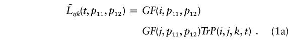The symbol in equation (1a) is used to distinguish the likelihoods for TDT_std from the likelihoods for TDT_ae. Because we assume that there are no errors, the recoded genotypes (i,j,k) are all consistent (see table 1). An important consequence of this simplification is that the log likelihood of equation (1a) reduces to

Through examination of equation (1b), we note that maximizing over the parameter t is independent of maximizing over the parameters p₁₁ and p₁₂. Therefore, when considering the overall log likelihood of the data set, which is given by the formula

and considering the difference of log likelihoods,

it follows from equation (1b) that and, in fact, the difference (eq. [3a]) is actually independent of the parameters p₁₁ and p₁₂. With this understanding, we may rewrite equation (3a) as

We shall refer to the value of equation (3b) as TDT_std. Through use of standard calculus techniques, it is possible to solve for the MLE in terms of the number of different observed trios N_ijk. Let

Through use of this notation, the value of t that maximizes the log likelihood in equation (3b) is

This value of t is used when computing the test statistic TDT_std.

Simulations

The data selected for use with the TDT tests consisted of an SNP locus that has two alleles in the population. These alleles were coded as “1” and “2.” Each replicate of each simulation consisted of genotype data from a number of trios (father, mother, and affected child). We simulated genotype data under two models: the null model, in which there was neither linkage nor LD, and the power model, in which the SNP marker locus was linked to the disease locus and there was LD between the marker and the disease locus. We assumed that the disease locus also has two alleles. For the null simulations, we set a recombination fraction (θ) of .5 between marker and disease, and we assumed that all loci were in Hardy-Weinberg equilibrium, so that two-locus haplotype frequencies were just the products of the allele frequencies at each of the two loci. For the power simulations, two-locus haplotype frequencies were completely determined by the allele frequencies at each of the two loci and by an additional parameter, D′. The value D′ is related to Lewontin's (1964) D, by the formula D^′=D/min(p₊p₂,p_dp₁), where p₊ and p_d were the allele frequency of the wild-type allele and the disease allele, respectively, at the disease locus, and p₁ and p₂ were the allele frequencies of the 1 allele and 2 allele, respectively, at the SNP marker locus. The values of D′ considered for these simulations were .5 and .8. From this point forward, the term “m% LD” (meaning “the %LD is m%”) for some integer m and some power simulation means that D^′=.01×m. For example, 20% LD means that D^′=.2.

In all power simulations, we assumed that disease locus and marker locus were completely linked (θ=0). We assert that this assumption is reasonable, given the dense coverage that SNPs have throughout the human genome (Chakravarti 1999).

For both the null and power simulations, we considered sample sizes of 100 and 500 trios. Allele frequencies for the marker locus were set either at .5 each (equal allele frequencies) or at .25 for the 1 allele in all simulations. For the LD simulations, we considered allele frequencies of .001 (rare) and .2 (common) for the disease (non–wild type) allele. As above, we used the notations “+” and “d” to refer to the wild-type and disease alleles, respectively, at the disease locus.

Genotype data for the null simulations were created by SIMULATE (Terwilliger and Ott 1994; SIMULATE ftp site), and data for the power simulations were created by FASTSLINK (Ott 1989; Weeks et al. 1990; Statgen Software Web site). For the power simulations, there were two modes of inheritance for the disease locus: recessive (a fully penetrant recessive model with no phenocopies), and dominant (a reduced-penetrance dominant model, in which the penetrance of each of the genotypes [at the disease locus] +d and dd was .6, and the penetrance of the genotype ++ was .02). The recessive disease model was chosen because it has been shown (Terwilliger and Ott 1992) that the TDT statistic is most powerful for such a disease model. The dominant disease locus model was chosen to reflect a more “realistic” disease model for complex diseases.

The pairs of error rates (ɛ₁, ɛ₂) we assumed for the marker locus were (.01, .01), (.01, .05), (.05, .01), (.05, .05), (.05, .10), and (.10, .05). We chose these pairs to provide a sense of the performance of the test statistics under a broad range of error rates. Errors were introduced randomly and independently into the genotype data files, by means of a computer program. For each simulation, the proportion of trios that showed consistency was recorded. In table 3, we report the average proportion of trios (over 1,000 replicates) that showed consistency.

Table 3.

Results of Null Simulations

					Type I Error Rate
					TDTae		TDTstda
No. ofTrios	1-Allele Frequency	ɛ1	ɛ2	AverageProportion ofConsistentPedigrees	5% Level	1% Level	5% Level	1% Level
100	.25	.01	.01	.984	.054	.006	.051	.011
100	.25	.01	.05	.941	.051	.010	.102	.024
100	.25	.05	.01	.969	.061	.005	.085	.028
100	.25	.05	.05	.929	.042	.009	.112	.036
100	.25	.05	.10	.887	.052	.011	.174	.068
100	.25	.10	.05	.913	.055	.014	.185	.063
100	.50	.01	.01	.985	.046	.009	.065	.012
100	.50	.01	.05	.958	.055	.009	.056	.007
100	.50	.05	.01	.958	.046	.015	.040	.006
100	.50	.05	.05	.935	.053	.009	.061	.009
100	.50	.05	.10	.906	.054	.015	.059	.014
100	.50	.10	.05	.906	.042	.009	.059	.016
500	.25	.01	.01	.984	.052	.013	.078	.022
500	.25	.01	.05	.942	.048	.008	.268	.118
500	.25	.05	.01	.969	.058	.012	.163	.047
500	.25	.05	.05	.928	.048	.008	.411	.201
500	.25	.05	.10	.886	.045	.009	.606	.395
500	.25	.10	.05	.912	.052	.011	.631	.386
500	.50	.01	.01	.985	.052	.012	.067	.010
500	.50	.01	.05	.958	.046	.010	.056	.014
500	.50	.05	.01	.959	.042	.008	.055	.006
500	.50	.05	.05	.932	.052	.014	.041	.008
500	.50	.05	.10	.904	.046	.010	.063	.010
500	.50	.10	.05	.905	.058	.012	.060	.011

^aValues in boldface italics have 95% CIs that do not contain a set level of significance (5%, 1%), based on the method for establishing CIs (see Results section, Null Simulations).

Throughout this article, the terms “type I error rate” and “power,” at the α% level of significance for a particular statistic, mean the proportion of replicates for a particular null or power simulation, respectively, that exceed χ²₁(.01×α), where χ²₁(.01×α) refers to the (two-sided) cutoff for a χ² statistic with 1 df. The type I error rate at the 5% and 1% levels of significance are reported for null simulations in table 3, and the power at the 5% and 1% levels of significance are reported for power simulations in tables 4 and 5.

Table 4.

Results of Power Simulations with TDT_ae for a Fully Penetrant Recessive Disease Model, 50% LD, and a .001 Disease-Allele Frequency

				Power
No. ofTrios	1-Allele Frequency	ɛ1	ɛ2	5% Level	1% Level
100	.25	.01	.01	.916	.742
100	.25	.01	.05	.768	.528
100	.25	.05	.01	.879	.681
100	.25	.05	.05	.749	.500
100	.25	.05	.10	.537	.302
100	.25	.10	.05	.660	.419
100	.50	.01	.01	1.000	.995
100	.50	.01	.05	.999	.981
100	.50	.05	.01	.999	.988
100	.50	.05	.05	.990	.956
100	.50	.05	.10	.950	.858
100	.50	.10	.05	.972	.904
500	.25	.01	.01	1.000	1.000
500	.25	.01	.05	1.000	.999
500	.25	.05	.01	1.000	1.000
500	.25	.05	.05	.999	.998
500	.25	.05	.10	.990	.958
500	.25	.10	.05	.999	.992
500	.50	.01	.01	1.000	1.000
500	.50	.01	.05	1.000	1.000
500	.50	.05	.01	1.000	1.000
500	.50	.05	.05	1.000	1.000
500	.50	.05	.10	1.000	1.000
500	.50	.10	.05	1.000	1.000

Table 5.

Results of Power Simulations with TDT_ae for a Reduced Penetrance Dominant Model, 80% LD, and a .001 Disease-Allele Frequency

				Power
No. ofTrios	1-Allele Frequency	ɛ1	ɛ2	5% Level	1% Level
100	.25	.01	.01	.169	.075
100	.25	.01	.05	.116	.037
100	.25	.05	.01	.154	.060
100	.25	.05	.05	.129	.039
100	.25	.05	.10	.097	.033
100	.25	.10	.05	.117	.031
100	.50	.01	.01	.404	.190
100	.50	.01	.05	.335	.165
100	.50	.05	.01	.398	.193
100	.50	.05	.05	.287	.124
100	.50	.05	.10	.228	.097
100	.50	.10	.05	.243	.092
500	.25	.01	.01	.602	.301
500	.25	.01	.05	.377	.160
500	.25	.05	.01	.542	.282
500	.25	.05	.05	.356	.161
500	.25	.05	.10	.276	.107
500	.25	.10	.05	.330	.151
500	.50	.01	.01	.985	.927
500	.50	.01	.05	.962	.809
500	.50	.05	.01	.975	.854
500	.50	.05	.05	.928	.713
500	.50	.05	.10	.774	.577
500	.50	.10	.05	.834	.628

Maximization over Three Parameters for Power Simulations

Although it is possible to maximize the likelihood equation (2) over all five parameters, the process is computationally intensive. Therefore, for our power simulations (tables 4 and 5), we assumed that we knew the values of the error rates ɛ₁ and ɛ₂ used to generate errors and only maximized the log-likelihood equation (2) over, at most, three parameters. It is true that this assumption has the potential effect of increasing the power of the TDT_ae for these simulations, but comparisons of the power from the TDT_ae maximizing over three parameters versus five parameters did not show an appreciable increase in power in favor of the three-parameter simulations (data not shown), whereas the reduction in computation time was appreciable (a factor of 9²).

Power Comparison

The TDT_ae statistic has the advantage of allowing for errors in the analysis of SNP genotype data, but at the computational cost of maximizing over five parameters (all parameters but t are nuisance parameters), in contrast to the TDT_std, which maximizes over one parameter. In theory, both statistics are asymptotically disturbed as χ²₁ and, given a dense enough grid search, there is no difference in power between the two methods. In practice, however, the exact maximum likelihood for the TDT_ae is most likely not achieved when maximizing over the five parameters, because of computational limitations. For the TDT_std, the maximum likelihood is always achieved through use of the value of in equation (4).

To assess the effect that maximization over an additional four parameters has on the power of the TDT_ae, we performed power simulations in which there are no errors in the genotype data created. Each simulation is determined by two factors: the number of trios simulated (100, 200, 500, and 1000) and the 1-allele frequency at the marker locus (.25, .50). In all simulations, the disease-allele frequency (p_d) was .20, θ between the disease and the marker locus was 0, and the %LD was 50. For each simulated data set (replicate) in each simulation, the TDT_std and TDT_ae were computed as described above. A total of 250 replicates were created and analyzed for each simulation. Power curves for each method are presented in figure 1.

Figure 1.

Average power for the TDT_std and TDT_ae statistics, for errorless data sets in which the 1-allele frequency = .25, p_d=.2, and %LD = 50, and for which the disease-locus model is a fully penetrant recessive locus. Each average is computed over 250 replicates. The suffixes “-std” and “-ae” in the Significance Level legend indicate power for the TDT_std and TDT_ae statistics, respectively.

Results

Null Simulations

Table 3 presents a summary of the results for our null simulations. Each row records the number of trios considered, the error rates ɛ₁ and ɛ₂, the frequency of the 1 allele at the marker locus, the average proportion of consistent trios in each replicate (averaged over 1,000 replicates), and the type I error rates at the 5% and 1% levels of significance for the TDT_ae and TDT_std statistics. We indicate, in boldface italic type, those simulations for which the 95% confidence interval (CI) (Fisher 1960) of the type I error rate does not include the chosen significance level, indicating that the test statistic showed an inflation in type I error for this particular simulation.

From studying table 3, we see that the TDT_ae statistic maintains a correct type I error rate in all simulations, for each of the significance levels (5% and 1%). On the other hand, the TDT_std statistic shows an inflation in the type I error rate for a number of simulations. In fact, with the exception of the (.01, .01) pair of error rates, the TDT_std always shows inflation in type I error when the 1-allele frequency is .25. As a way of comparing the increases in type I error across different levels of significance, we consider the ratios (type I error rate at 5% level)/.05 and (type I error rate at 1% level)/.01. The largest ratio occurs for 500 trios, a 1-allele frequency of .25, the pair of error rates (.10, .05), and a significance level of 1%. Under these conditions, we see a ratio of 38.6, an ∼40-fold increase in type I error.

For the equal allele frequency case (1-allele frequency = .5), the TDT_std statistic shows a small inflation in the type I error rate when the pair of error rates is (.01, .01), for both the 100- and the 500-trio case. However, it maintains a correct type I error rate for all other simulations of the equal allele frequency case. We hypothesize that, for our error model, TDT_std maintains a correct type I error rate only when marker-allele frequencies are equal.

Intuitively, the reason for an increase in type I error rate for the TDT_std test statistic for unequal allele frequencies seems clear. When the allele frequencies are more divergent—as opposed to more equal—there are more trios in which both parents are homozygous. When errors are introduced into trios in which both parents are homozygous and the resultant trio is consistent, the observed (and incorrect) trio of genotypes is counted in the estimation of the parameter t, introducing a bias in t away from its true value of .5. In addition, although it seems counterintuitive that the TDT_std type I error rates are so much greater for a larger sample than for a smaller one, we comment that, even though the percentage of trios that show Mendelian consistency is the same, on average, for the same error rates in the 100- or 500-trio cases, the actual number of trios that have errors and that show Mendelian consistency is approximately five times as large in the 500-trio case as in the 100-trio case. As mentioned above, when marker-allele frequencies are unequal, a significant number of these trios (specifically, the trios in which true homozygous parents are incorrectly coded as heterozygous) will be counted in the estimation of the parameter t. For the 500-trio case, we expect that five times as many such trios are counted as for the 100-trio case, thus increasing the type I error rate, as was observed in the simulation results.

Because of the significant and consistent increase in type I error rate of the TDT_std statistic for unequal allele frequencies, we conclude that it is not a useful test in the presence of errors. For our power simulations, we therefore focus on the TDT_ae statistic. Finally, we note that, for all simulations considered, the average proportion of trios that display consistency is ⩾88%, and this average increases to 93% when error rates of ⩽.05 are considered.

Power Simulations

Here we present tables for some of our simulations and discuss results for all of the simulations. The number of tables has been reduced, to conserve space. Table 4 provides simulation results for the fully penetrant recessive disease model with 50% LD and a .001 disease-allele frequency. Table 5 presents simulation results for the reduced-penetrance dominant disease with 80% LD and a .001 disease-allele frequency.

In studying these two tables, we notice some common patterns. First, we notice, for each sample size (100 or 500 trios) and each set of allele frequencies (1-allele frequency = .25 or .5), that, as the values of ɛ₁ and ɛ₂ increase, the power of the TDT_ae statistic decreases. This decrease due to larger error rates is to be expected, since an increase in the value of the error rates decreases the probability that any single true trio of genotypes is associated with a given observed trio of genotypes. With regard to specific error rates, it is interesting to note that power was reduced most when ɛ₂ was largest—that is, when error was introduced into the 2 allele, which is the allele in coupling with the disease allele d. A second observation is that, for each sample size and each pair of error rates, the power of the TDT_ae is greater when marker-allele frequencies are equal, as opposed to when the 1-allele frequency is .25. A third observation is that, particularly for the dominant mode of inheritance, to achieve any kind of power with the TDT_ae (say, power >.60), one needs large sample sizes (⩾500 trios) and small error rates. In fact, for sample sizes of 500 trios with a dominant mode of inheritance (table 5), power is >.6 at the 5% level for 7/12 simulations and at the 1% level for 5/12 simulations.

As mentioned in the Methods section, power simulations were also performed for the recessive mode of inheritance, in which the disease-allele frequency p_d was .20 and LD was 50%, as well as for conditions of 80% LD with two sets of disease-allele frequencies (p_d=.001 or .20). For the case of 50% LD, p_d=.20, power at the 5% level was .69–1.00, and power at the 1% level was .46–1.00. With one exception (100 trios, ɛ₁=.05 and ɛ₂=.10), power at the 5% and 1% levels was >.8 and >.62, respectively. When the sample size was 500 trios, all power (at the 5% and 1% levels) was >.99. For recessive simulations in which there was 80% LD, power at the 5% level was .93–1.00, and power at the 1% level was .78–1.00. As was the case for 50% LD and p_d=.20—with one exception (100 trios, ɛ₁=.05, ɛ₂=.10, p_d=.001)—power at the 5% and 1% levels was >.98 and >.93, respectively.

For those power simulations with a dominant mode of inheritance for the disease locus that are not reported in table 5 (50% LD with p_d=.001 or .20, and 80% LD with p_d=.20), we report the following ranges of power observed: for the case of 50% LD (p_d=.001 or .20), power at the 5% level was .07–.99, and power at the 1% level was .02–.98. In general, for sample sizes of 100 trios, power was low. In fact, the largest power observed at the 5% level for 100 trios was .60. For simulations in which there was 80% LD and p_d=.20, power at the 5% level was .19–1.00, and power at the 1% level was .03–1.00. As mentioned above, in all cases in which other variables (%LD, allele frequencies) were fixed, power was lowest when the error rates were largest.

An overall observation that can be made about the TDT_ae statistic on the basis of these simulations is that the factors that influence the power of this statistic are sample size, mode of inheritance of the disease locus, marker- and disease-allele frequencies, %LD, and, for this analysis, error rates ɛ₁ and ɛ₂. The same factors affect the power of the TDT_std (Xiong and Guo 1998); however, the addition of errors into genotype data has the adverse effect of decreasing the power in comparison with the power in the errorless data situation.

Power Comparison

Figure 1 presents the results of the power-comparison simulations. The vertical axis is the power at the α% level of significance for the TDT_std and TDT_ae statistics for simulations, considering four different numbers of trios: 100, 200, 500, and 1,000. What we glean from this graph is that, for this simulation, the difference in power is dependent on both the number of trios considered and the level of significance. The greatest power difference is almost .20 when there are 100 trios, and the level of significance is 0.10%. Note that, at the 5% level of significance, the greatest power difference is .05, when the number of trios is 100. Another observation made from this graph is that, when the sample size is large enough (⩾500), there is essentially no difference in power between the TDT_std and TDT_ae statistics.

We also performed simulations in which the marker-allele frequencies were equal. The result of those simulations was that there was no difference in power between the TDT_std and TDT_ae statistics, for any number of trios or any level of significance. Both statistics had a power of 1.0 for all simulations.

Summary and Discussion

The purposes of the present study included the assessment of the effects of genotyping errors on a particular TDT (TDT_std) and on a new TDT (TDT_ae) that allows for random genotyping errors in the analysis, the evaluation of power for the TDT_ae under a variety of scenarios, and a power comparison between the TDT_std and the TDT_ae, when no errors are present in the genotype data. The results indicated that the TDT_std, when applied to data that have been “cleaned” (i.e., data in which inconsistent trios are removed), does not maintain the correct type I error rate and that the type I error increases both with an increase in sample size and with an increase in the error rates ɛ_i(i∈{1,2}). In contrast to this, the TDT_ae statistic maintains a correct type I error rate for the simulations considered. The power of the TDT_ae is dependent on individual error rates, mode of inheritance at the disease locus, allele frequencies at the disease and marker locus, %LD, and sample size. Finally, we note that, for simulations in which no genotyping errors are introduced, the power of the TDT_std statistic is at least that of the TDT_ae statistic, but this difference in power decreases as the sample size increases.

It is important to note that the TDT_ae is designed for application to data sets in which inconsistent trios are observed. We comment that the TDT_ae probably does not maintain a correct type I error rate when applied to data in which inconsistent trios have been removed. Another way of saying this is that the TDT_ae statistic should be applied only to data sets that are “raw”—that is, data sets in which inconsistent trios (if any exist) are not removed when computing the test statistic.

An interesting result of the present study, although not its main focus, is that even when error rates are relatively high (ɛ₁,ɛ₂⩾.05), most (>88%) trios will display consistency (table 3). This finding agrees with the analytic solutions of Gordon et al. (1999a, 1999b). For example, Gordon et al. (1999a) showed that, for ɛ₁=ɛ₂=.05, on average, >90% of trios will show consistency when marker-allele frequencies are equal, there is no linkage between marker and disease locus, and the marker locus is in Hardy-Weinberg equilibrium.

The error model assumed in the present study is based on an assumption of random errors. A question that arises is whether this assumption is reasonable. For SNP data, this question will be answered more conclusively as more SNP genotype data are created and analyzed. From a statistical viewpoint, however, the real question is whether statistics like the TDT_ae are robust to different error models. This research is work in progress.

Because of the potential increase in power that haplotype methods have over single-locus methods (Dudbridge et al. 2000; Xiong et al. 2000) and because of the widespread use of microsatellite markers for linkage and LD analysis (e.g., Lee et al. 2001), a natural question to ask is whether the TDT_ae method can be extended to a test using multi-locus haplotypes and/or multi-allelic markers. Perhaps the main challenge of such extensions is the use of as few parameters for error rates as is possible. For example, with n alleles at a marker, the number of possible individual error rates ɛ_i is n(n-1). We suspect that, for highly polymorphic loci, the best approach may be the one recommended by Schaid (1996) and Spielman and Ewens (1998), which involves down-coding of alleles and performance of multiple two-allele tests. We plan to pursue this research.

Finally, we note that, as is the case with all statistics applied to genotype data, a reassessment of power would be needed for whole-genome scans. We plan to make software available shortly that computes the TDT_ae statistic. The code will be freely available.

References

- Akey JM, Zhang K, Xiong M, Doris P, Jin L (2001) The effect that genotyping errors have on the robustness of common linkage-disequilibrium measures. Am J Hum Genet 68:1447–1456 [DOI] [PMC free article] [PubMed] [Google Scholar]
- Box GEP, Hunter WG, Hunter JS (1978) Statistics for experimenters. John Wiley & Sons, New York [Google Scholar]
- Broman KW (1999) Cleaning genotype data. Genet Epidemiol 17 Suppl 1:S79–S83 [DOI] [PubMed] [Google Scholar]
- Brzustowicz LM, Merette C, Xie X, Townsend T, Gilliam C, Ott J (1993) Molecular and statistical approaches to the detection and correction of errors in genotype databases. Am J Hum Genet 53:1137–1145 [PMC free article] [PubMed] [Google Scholar]
- Buetow KH (1991) Influence of aberrant observations on high-resolution linkage analysis outcomes. Am J Hum Genet 49:985–994 [PMC free article] [PubMed] [Google Scholar]
- Chakravarti A (1999) Population genetics: making sense out of sequence. Nat Genet 21 Suppl:56–60 [DOI] [PubMed] [Google Scholar]
- Collins FS, Brooks LD, Chakravarti A (1998) A DNA polymorphism discovery resource for research on human genetic variation. Genome Res 8:1229–1231 [DOI] [PubMed] [Google Scholar]
- Douglas JA, Boehnke M, Lange K (2000) A multipoint method for detecting genotyping errors and mutations in sibling-pair linkage data. Am J Hum Genet 66:1287–1297 [DOI] [PMC free article] [PubMed] [Google Scholar]
- Dudbridge F, Koeleman BPC, Todd JA, Clayton DG (2000) Unbiased application of the transmission/disequilibrium test to multilocus haplotypes. Am J Hum Genet 66:2009–2012 [DOI] [PMC free article] [PubMed] [Google Scholar]
- Ehm MG, Kimmel M, Cottingham RW Jr (1996) Error detection for pedigree data, using likelihood methods. Am J Hum Genet 58:225–234 [PMC free article] [PubMed] [Google Scholar]
- Ewen KR, Bahlo M, Treloar SA, Levinson DF, Mowry B, Barlow JW, Foote SJ (2000) Identification and analysis of error types in high-throughput genotyping. Am J Hum Genet 67:727–736 [DOI] [PMC free article] [PubMed] [Google Scholar]
- Fisher RA (1960) The design of experiments. Oliver and Boyd, Edinburgh [Google Scholar]
- Ghosh S, Karanjawala ZE, Hauser ER, Ally D, Knapp JI, Rayman JB, Musick A, Tannenbaum J, Te C, Shapiro S, Eldridge W, Musick T, Martin C, Smith JR, Carpten JD, Brownstein MJ, Powell JI, Whiten R, Chines P, Nylund SJ, Magnuson VL, Boehnke M, Collins FS (1997) Methods for precise sizing, automated binning of alleles, and reduction in large-scale genotyping using fluorescently labelled dinucleotide markers: FUSION (Finland-US Investigation of NIDDM Genetics) study group. Genome Res 7:165–178 [DOI] [PubMed] [Google Scholar]
- Giordano M, Mellai M, Hoogendoorn B, Momigliano-Richiardi P (2001) Determination of SNP allele frequencies in pooled DNAs by primer extension genotyping and denaturing high-performance liquid chromatography. J Biochem Biophys Methods 47:101–110 [DOI] [PubMed] [Google Scholar]
- Goldstein DR, Zhao H, Speed TP (1997) The effects of genotyping errors and interference on estimation of genetic distance. Hum Hered 47:86–100 [DOI] [PubMed] [Google Scholar]
- Gordon D, Heath SC, Ott J (1999a) True pedigree errors more frequent than apparent errors for single nucleotide polymorphisms. Hum Hered 49:65–70 [DOI] [PubMed] [Google Scholar]
- Gordon D, Matise TC, Heath SC, Ott J (1999b) Power loss for multiallelic transmission/disequilibrium test when errors introduced: GAW11 simulated data. Genet Epidemiol 17 Suppl 1: S587–S592 [DOI] [PubMed] [Google Scholar]
- Gordon D, Ott J (2001) Assessment and management of single nucleotide polymorphism genotype errors in genetic association analysis. Pac Symp Biocomput 2001:18–29 [DOI] [PubMed] [Google Scholar]
- Göring HHH, Terwilliger JD (2000a) Linkage analysis in the presence of errors I: complex-valued recombination fractions and complex phenotypes. Am J Hum Genet 66:1095–1106 [DOI] [PMC free article] [PubMed] [Google Scholar]
- ——— (2000b) Linkage analysis in the presence of errors II: marker-locus genotyping errors modeled with hypercomplex recombination fractions. Am J Hum Genet 66:1107–1118 [DOI] [PMC free article] [PubMed] [Google Scholar]
- ——— (2000c) Linkage analysis in the presence of errors III: marker loci and their map as nuisance parameters. Am J Hum Genet 66:1298–1309 [DOI] [PMC free article] [PubMed] [Google Scholar]
- ——— (2000d) Linkage analysis in the presence of errors IV: joint pseudomarker analysis of linkage and/or linkage disequilibrium on a mixture of pedigrees and singletons when the mode of inheritance cannot be accurately specified. Am J Hum Genet 66:1310–1327 [DOI] [PMC free article] [PubMed] [Google Scholar]
- Heath SC (1998) A bias in TDT due to undetected genotyping errors. Am J Hum Genet Suppl 63:A292 [Google Scholar]
- Kendall MG, Stuart A, Ord JK (1991) Kendall's advanced theory of statistics, vol 2A, 2d ed. Oxford University Press, New York [Google Scholar]
- Lee MH, Gordon D, Ott J, Lu K, Ose L, Miettinen T, Gylling H, Stalenhoef AF, Pandya A, Hidaka H, Brewer B Jr, Kojima H, Sakuma N, Pegoraro R, Salen G, Patel SB (2001) Fine mapping of a gene responsible for regulating dietary cholesterol absorption: founder effects underlie cases of phytosterolaemia in multiple communities. Eur J Hum Genet 9:375–384 [DOI] [PMC free article] [PubMed] [Google Scholar]
- Lewontin RC (1964) The interaction of selection and linkage. I. General considerations: heterotic models. Genetics 49:49–67 [DOI] [PMC free article] [PubMed] [Google Scholar]
- Lincoln SE, Lander ES (1992) Systematic detection of errors in genetic linkage data. Genomics 14:604–610 [DOI] [PubMed] [Google Scholar]
- Lunetta KL, Boehnke M, Lange K, Cox DR (1995) Experimental design and error detection for polyploid radiation hybrid mapping. Genome Res 5:151–163 [DOI] [PubMed] [Google Scholar]
- Matise TC (1995) Genome scanning for complex disease genes using the transmission/disequilibrium test and haplotype-based haplotype relative risk. Genet Epidemiol 12:641–645 [DOI] [PubMed] [Google Scholar]
- O'Connell JR, Weeks DE (1998) PedCheck: a program for identification of genotype incompatibilities in linkage analysis. Am J Hum Genet 63:259–266 [DOI] [PMC free article] [PubMed] [Google Scholar]
- ——— (1999) An optimal algorithm for automatic genotype elimination. Am J Hum Genet 65:1733–1740 [DOI] [PMC free article] [PubMed] [Google Scholar]
- Ott J (1977) Linkage analysis with misclassification at one locus. Clin Genet 12:110–124 [DOI] [PubMed] [Google Scholar]
- ——— (1989) Computer-simulation methods in human linkage analysis. Proc Natl Acad Sci USA 86:4175–4178 [DOI] [PMC free article] [PubMed] [Google Scholar]
- ——— (1993) Detecting marker inconsistencies in human gene mapping. Hum Hered 43:25–30 [DOI] [PubMed] [Google Scholar]
- Risch N, Merikangas K (1996) The future of genetic studies of complex human diseases. Science 273:1516–1517 [DOI] [PubMed] [Google Scholar]
- Schaid DJ (1996) General score tests for associations of genetic markers with disease using cases and their parents. Genet Epidemiol 13:423–449 [DOI] [PubMed] [Google Scholar]
- Schork NJ, Fallin D, Thiel B, Xu X, Broeckel U, Jacob HJ, Cohen D (2001) The future of genetic case-control studies. Adv Genet 42:191–212 [DOI] [PubMed] [Google Scholar]
- Sham P (1998) Statistics in human genetics. J Wiley & Sons, New York [Google Scholar]
- Shields DC, Collins A, Buetow KH, Morton NE (1991) Error filtration, interference, and the human linkage map. Proc Natl Acad Sci USA 88:6501–6505 [DOI] [PMC free article] [PubMed] [Google Scholar]
- Spielman RS, Ewens WJ (1998) A sibship test for linkage in the presence of association: the sib transmission/disequilibrium test. Am J Hum Genet 62:450–458 [DOI] [PMC free article] [PubMed] [Google Scholar]
- Spielman RS, McGinnis RE, Ewens WJ (1993) Transmission test for linkage disequilibrium: the insulin gene region and insulin-dependent diabetes mellitus (IDDM). Am J Hum Genet 52:506–516 [PMC free article] [PubMed] [Google Scholar]
- Stringham HM, Boehnke M (1996) Identifying marker typing incompatibilities in linkage analysis. Am J Hum Genet 59:946–950 [PMC free article] [PubMed] [Google Scholar]
- Terwilliger J, Ott J (1992) A haplotype-based ‘haplotype relative risk' approach to detecting allelic associations. Hum Hered 42:337–346 [DOI] [PubMed] [Google Scholar]
- ——— (1994) Handbook of human genetic linkage. Johns Hopkins University Press, Baltimore [Google Scholar]
- Terwilliger JD, Weeks DE, Ott J (1990) Laboratory errors in the reading of marker alleles cause massive reductions in lod score and lead to gross overestimates of the recombination fraction. Am J Hum Genet Suppl 47:A201 [Google Scholar]
- Xiong M, Akey J, Jin L (2000) The haplotype linkage disequilibrium test for genome-wide screens: its power and study design. Pac Symp Biocomput 2000:675–686 [DOI] [PubMed] [Google Scholar]
- Xiong M, Guo SW (1998) The power of linkage detection by the transmission disequilibrium tests. Hum Hered 48:295–312 [DOI] [PubMed] [Google Scholar]
- Wang DG, Fan JB, Siao CJ, Berno A, Young P, Sapolsky R, Ghandour G, et al (1998) Large-scale identification, mapping, and genotyping of single-nucleotide polymorphisms in the human genome. Science 280:1077–1082 [DOI] [PubMed] [Google Scholar]
- Weeks DE, Ott J, Lathrop GM (1990) SLINK: a general simulation program for linkage analysis. Am J Hum Genet Suppl 47:A204 [Google Scholar]